Age of Information and Mobility
by
Vishrant Tripathi
B.Tech., Electrical Engineering
Indian Institute of Technology Bombay, 2017
Submitted to the Department of Electrical Engineering and Computer
Science
in partial fulfillment of the requirements for the degree of
Master of Science in Electrical Engineering and Computer Science
at the
MASSACHUSETTS INSTITUTE OF TECHNOLOGY
June 2019
c
○ Massachusetts Institute of Technology 2019. All rights reserved.
Author . . . .
Department of Electrical Engineering and Computer Science
May 23, 2019
Certified by . . . .
Eytan Modiano
Professor of Aeronautics and Astronautics
Thesis Supervisor
Accepted by. . . .
Leslie A. Kolodziejski
Professor of Electrical Engineering and Computer Science
Age of Information and Mobility
by
Vishrant Tripathi
Submitted to the Department of Electrical Engineering and Computer Science on May 23, 2019, in partial fulfillment of the
requirements for the degree of
Master of Science in Electrical Engineering and Computer Science
Abstract
Age of information is a recently proposed metric that measures the freshness of in-formation at a destination receiving data from an inin-formation source. It has become popular in the networking and queuing community, especially for studying delivery of real time status updates. In this thesis, we explore applications of AoI to mobile and adhoc networks. More specifically, we look at two problems - 1) Age optimal information collection and dissemination from locations arranged on a graph, using a mobile agent that travels between them, and 2) Age-based transmission schemes for a group of mobile agents which need to continuously exchange information while moving around in a cell partitioned network. We also derive expressions for age met-rics for discrete time queuing systems under various service disciplines, and service and arrival time distributions.
Thesis Supervisor: Eytan Modiano
Acknowledgments
First and foremost, I am thankful to Prof. Eytan Modiano for giving me the time and freedom to work on problems that I find interesting; and providing crucial help and guidance, whenever I got stuck. His expertise, advice, and careful attention to detail were essential to the completion of this thesis and are much appreciated.
I would like to thank Rajat Talak, for many useful discussions from high level problem formulations to low level nitty-gritties. A large part of this thesis is based on work that we did in collaboration. I am also thankful to Igor Kadota - I have bugged him too many times over the past two years to discuss ideas, proof techniques and research in general.
I sincerely thank people at MIT who have made my life in graduate school very enjoyable - friends from MIT Cricket Club for dragging me outdoors every once in a while and the Ashdown Coffee Hour Committee for being a reliable source of fresh fruit and lively discussion all year round. I am thankful to my friends from CNRG who I have shared an office with: Xinzhe Fu, Bai Liu, Anurag Rai, Thomas Stahlbuhk, Jianan Zhang, Qingkai Liang, Ertem Nusret, Georgia Dimaki, and Xinyu Wu. I woud also like to acknowledge my flatmates Aniket Patankar and German Parada for being the best flatmates one can ever hope for.
Finally, I would like to thank my parents Sheela and Vipul Tripathi, for being a constant source of support and encouragement. I know that this thank you note does not do justice to everything they have done for me over the years. None of this would have been possible without their love and belief in me. Thank you for everything!
Contents
1 Introduction 13
1.1 Motivation for Age of Information . . . 15
1.2 Metrics for Age of Information . . . 16
1.3 AoI for discrete time Queues . . . 16
1.4 Mobility on a Graph . . . 18
1.4.1 Related Work . . . 19
1.5 AoI in Mobile Ad-Hoc Networks . . . 20
1.5.1 Related Work . . . 20
1.6 Outline and Contributions . . . 22
2 AoI for Discrete Time Queues 25 2.1 Relating Continuous and Discrete AoI . . . 25
2.2 Geo/G/1 Queue . . . 29
2.3 Geo/G/1 Queue with Vacations . . . 30
2.4 LCFS Queues . . . 34
3 Mobility on a Graph 37 3.1 System Model . . . 37
3.1.2 Trajectory Space . . . 42
3.2 Information Gathering . . . 42
3.2.1 Randomized Trajectories . . . 43
3.2.2 Peak Age Minimization . . . 46
3.2.3 Average Age Minimization . . . 51
3.2.4 A Heuristic Randomized Trajectory . . . 54
3.2.5 Age-based Trajectories . . . 60
3.3 Information Dissemination . . . 63
3.3.1 Age for Ber/G/1 Queue with Vacations . . . 65
3.3.2 Age Minimization Problem . . . 68
3.4 Simulation Results . . . 72
3.5 Conclusions and Future Work . . . 76
4 AoI in Mobile Ad-hoc Networks 79 4.1 Single Source Model . . . 79
4.1.1 Policy . . . 81
4.1.2 Age Analysis . . . 81
4.2 Multiple Sources . . . 87
4.2.1 Policy . . . 88
4.3 Simulation Results . . . 89
4.4 Conclusions and Future Work . . . 93
A 95 A.1 Proof for Average Age in Theorem 2 . . . 95
A.2 Proof of Lemma 4 . . . 97
List of Figures
1-1 Age 𝐴(𝑡) evolution with time 𝑡 for an active source with inter-update intervals 𝐻1, 𝐻2, 𝐻3, and so on. . . 14
1-2 Age 𝐴(𝑡) evolution with time 𝑡 for an uncontrollable source with packet generation times 𝑡1, 𝑡2, 𝑡3, ... and packet delivery times 𝑡′1, 𝑡′2, 𝑡′3, ... . 15
2-1 Age 𝐴(𝑡) evolution over time 𝑡 along with the corresponding contin-uous age process. 𝑋𝑖 are inter-arrival times, 𝑆𝑖 are service times for
packet 𝑖. . . 27 2-2 Average age for geometrically distributed server times with probability
𝜇 = 0.75. We compare vacations with geometric, uniform bounded, and deterministic distributions having the same mean as it varies from 1 to 7. Solid lines represent arrival probability 𝜆 = 0.3 and dashed lines represent 𝜆 = 0.6. . . 33 2-3 Age 𝐴(𝑡) evolution in time 𝑡 for an LCFS queue with preemption. . . 34 3-1 Information gathering problem: time evolution of age 𝐴𝑖(𝑡); 𝐻𝑘,𝑖 is
3-2 Information dissemination problem: time evolution of age 𝐴𝑖(𝑡); 𝑡𝑘, 𝑡′𝑘
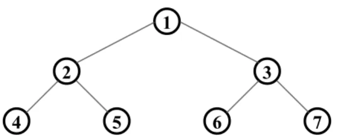
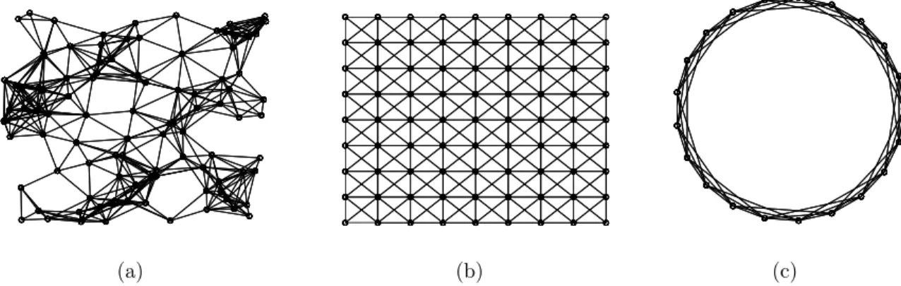
are the generation and reception times of the 𝑘th status update for terminal 𝑖. . . 40 3-3 Mobility graph restricted to a binary tree. . . 61 3-4 (a) A random geometric graph with 100 nodes, (b) A grid graph with
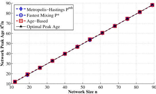
81 nodes and diagonal edges, and (c) A 3-connected ring or cycle graph with 21 nodes. . . 73 3-5 Information gathering problem in 𝒢(𝑛, 2/√𝑛): network peak age as
a function of network size 𝑛 for several proposed trajectories of the mobile agent. . . 74 3-6 Information gathering problem in 𝒢(𝑛, 2/√𝑛): network average age
as a function of network size 𝑛 for several proposed trajectories of the mobile agent. We average over 10 random graphs for each value of 𝑛. 75 3-7 Information gathering problem in the Grid graph: network average
age as a function of network size 𝑛 for several proposed trajectories of the mobile agent. . . 76 3-8 Information gathering problem in the Ring graph: network average
age as a function of network size 𝑛 for several proposed trajectories of the mobile agent. . . 77 3-9 Network average age as a function of network size . . . 77 4-1 In this example 𝑁 = 12 and 𝐶 = 36. The red cell is the source, while
the green cell is the destination, and the dots represent locations of mobile nodes at a particular time instant. . . 80
4-2 Average Age at the destination as a function of number of mobile nodes, for the constant density regime. We fix 𝑁/𝐶 = 2.5 nodes per cell . . . 89 4-3 Average Age at the destination as a function of number of mobile
nodes, for the sparse density regime. We fix 𝐶 = Θ(𝑁1.25) . . . . 90
4-4 Average Age at the destination as a function of number of mobile nodes, for the dense regime. We fix 𝐶 = Θ(𝑁0.833) . . . . 90
4-5 Network Average Age as a function of number of cells in the network for the 2 source case. We fix 𝑁 = 2 and compare the greedy policy with a randomized policy. . . 91 4-6 Network Average Age as a function of number of mobile nodes in the
network. We fix the number of cells 𝐶 = 100 and compare the greedy policy with a randomized policy. . . 92
Chapter 1
Introduction
Consider a system in which a source generates updates that traverse a network to reach the destination. The goal of the system is to ensure that the destination gets fresh information. Age of information (AoI), a destination centric metric of information freshness, was first introduced in [1]. It measures the time that has elapsed since the last received fresh update was generated at the source. Over the past few years, a rapidly growing body of work has analyzed AoI for various queuing systems [1–10] and wireless networks [11–17].
Throughout this work, we assume a discrete-time slotted system. Depending on the setting, we consider active sources which can generate fresh packets in ev-ery time-slot, as well as uncontrollable sources which generate packets accord-ing to some random process. The age process 𝐴(𝑡) at any destination increases by 1 in every time-slot in which it does not
Time (slotted) Age Process H1 1 H1 H3 H2 New update delivered Age A(t) H3
Figure 1-1: Age 𝐴(𝑡) evolution with time 𝑡 for an active source with inter-update intervals 𝐻1, 𝐻2, 𝐻3, and so on.
receive a useful update. For every useful update, the age drops to the amount of the time that has elapsed since the delivered update was generated at the source.
We track the age process 𝐴(𝑡) as the value of AoI at the beginning of every time-slot. Assume that the 𝑖th packet is generated at time 𝑡𝑖. Then, 𝐴(𝑡) satisfies the
following recursion 𝐴(𝑡 + 1) = ⎧ ⎪ ⎨ ⎪ ⎩ 𝐴(𝑡) + 1, if no delivery at time 𝑡 min{𝑡 − 𝑡𝑖, 𝐴(𝑡)} + 1, if 𝑖 is delivered.
Note that for an active source, the age always drops to 1 upon delivery of an update, since only the most recent update is delivered. See Figures 1-1 and 1-2 for examples of age evolution for active and uncontrollable sources.
t1' Age A(t) Time (slotted) Age Process t1 t2 t2' t3 t3' t4 t4' t1' t1 New update delivered t3' t3 t1' t1 + 1 t3' t3 + 1
Figure 1-2: Age 𝐴(𝑡) evolution with time 𝑡 for an uncontrollable source with packet generation times 𝑡1, 𝑡2, 𝑡3, ... and packet delivery times 𝑡′1, 𝑡′2, 𝑡′3, ...
1.1
Motivation for Age of Information
Age of information is extremely useful as a metric for freshness in networks where the main concern is real time delivery of status updates. There has been a rapidly growing body of literature applying AoI as a metric of interest to various networking applications, e.g. cache updating [18], networked control systems [19,20], networks with real-time traffic such as wireless sensor networks or real time processing in augmented and virtual reality systems, [12–17,21,22], and vehicular networks [11].
AoI is a distinct notion from throughput and delay, the more traditional QoS metrics used in networking literature. and leads to different scheduling policies as compared to schemes that attempt to minimize throughput and delay. We will see this in detail later.
1.2
Metrics for Age of Information
It is common in AoI literature to look at both peak age and average age. The peak age 𝐴p for an age process 𝐴(𝑡) is the time average of its peak values. Observe that
the age process 𝐴(𝑡) reaches peak in the time-slot that it receives a useful packet delivery, since the age drops in the next time-slot. Thus, the expression for peak age is given by 𝐴p, lim sup 𝑇 →∞ 𝑡=𝑇 ∑︀ 𝑡=1
𝐴(𝑡)1{update delivered at time 𝑡} 𝑡=𝑇
∑︀
𝑡=1
1{update delivered at time 𝑡}
.
The average age 𝐴ave is just the time average of the entire age process, and is given
by the following expression
𝐴ave, lim sup
𝑇 →∞ 1 𝑇 𝑇 ∑︁ 𝑡=1 𝐴(𝑡).
In the next section we discuss the difference between AoI for discrete time systems as we have introduced above and AoI for continuous time system, as is common in literature.
1.3
AoI for discrete time Queues
As discussed earlier, age of information (AoI) has been analyzed for a large variety of queuing systems over the past few years. Here, we provide a brief survey of these results. AoI was first studied for the first come first serve (FCFS) M/M/1, M/D/1, and D/M/1 queues in [1]. AoI for M/M/2 and M/M/∞ was studied in [2,3], in order to demonstrate the advantage of having parallel servers. In [8], age was analyzed for
parallel last come first serve (LCFS) servers, with preemptive service. Age analysis for queues with packet deadlines, in which a packet deletes itself after its deadline expiration, is considered in [9,10,23]. In [24], age has been analyzed under packet transmission errors. In [4], AoI for the LCFS queue with Poisson arrivals and Gamma distributed service was considered. In [5,6], the LCFS queue scheduling discipline, with preemptive service, is shown to be age optimal, when the service times are exponentially distributed.
More recently, a complete characterization of age distribution for FCFS and LCFS queues, with and without preemption, was done in [7,25]. In [26], it is proved that a heavy tailed service minimizes age for LCFS queue under preemptive service and the G/G/∞ queue.
As is evident from the literature, AoI has thus far been analyzed in detail for con-tinuous time queuing models. Discrete time queuing systems often arise in practice, especially in wireless networks [15], and are the focus of this thesis. In [15], the au-thors derived peak and average age expressions for the discrete time FCFS G/Geo/1 queue. The result lead to the derivation of separation principle in scheduling and rate control for age minimization in wireless networks.
In Chapter 2, we analyze age metrics for various discrete time queuing models using the results and analytical tools developed in [7,25,26]. We first consider the FCFS Geo/G/1 queue, with and without vacations. When taking vacations, we note that taking deterministic vacations, is the best resort towards minimizing age. We then derive peak and average age expressions for the discrete time LCFS G/G/1 with preemptive service. We build upon proof techniques from earlier results [15,26,27], and find that observations from the continuous time scenario carry forward to the discrete time scenario.
of this thesis and discuss related works in literature.
1.4
Mobility on a Graph
Many emerging applications depend on the collection and delivery of status up-dates between a set of ground terminals and a central terminal using mobile agents. Examples include: measuring traffic at road intersections [28], temperature, and pol-lution in cities [29], ocean monitoring using underwater autonomous vehicles [30], and surveillance using UAVs [31]. All of these applications depend upon regular sta-tus updates, that are communicated in a timely manner, so as to keep the central terminal and the ground terminals updated with fresh information.
Age of Information (AoI), the metric described earlier, captures timeliness of re-ceived information [1,15,32]. Unlike packet delay, AoI measures the lag in obtaining information at the destination node, and is therefore suited for applications involving gathering or dissemination of time sensitive updates. Age of information, at a desti-nation, is defined as the time that elapsed since the last received information update was generated at the source. AoI, upon reception of a new update packet, drops to the time elapsed since generation of the packet, and grows linearly otherwise.
We consider the problem of AoI minimization in gathering and dissemination of information updates, between a set of ground terminals and a central terminal. The information updates can be as small as a single packet containing temperature information or a high fidelity image or a video file. The ground terminals are equipped with low power transmitters, and a mobile agent is used to gather and disseminate information.
The age or freshness of information gathered and disseminated depends on the trajectory of the mobile agent, whose mobility is constrained to a mobility graph
𝐺 = (𝑉, 𝐸). The mobile agent can move from ground terminal 𝑖 to ground terminal 𝑗 only if (𝑖, 𝑗) ∈ 𝐸. This model can be used to capture the fact that the agent may not be able to move between any arbitrary locations due to topological limitations. We discuss the system model and our results in detail in Chapter 3.
1.4.1
Related Work
The problem of persistent monitoring in dynamic environments has been considered in [33–35] using tools from optimal control. These works focus on minimizing uncer-tainty when source locations are time varying, rather than timely monitoring over a fixed set of locations. There is also a large body of work focused on planning trajecto-ries for a mobile agent to optimize traditional performance metrics in wireless sensor networks; primarily throughput, delay and network lifetime; by leveraging variants of the Travelling Salesman Problem (TSP) [36–40]. We observe connections to this line of work, when we establish the optimality of a Hamiltonian cycle trajectory in a symmetric setting.
Optimal sampling trajectories for signals using mobile agents have been con-sidered in [41] and [42]. However, these works deal with sampling rates and perfect reconstruction of time invariant fields rather than freshness of information for sources generating real-time updates.
Closer to our work in this thesis are [43] and [44], in which some approximation trajectories to minimize maximum latency on metric graphs were proposed. In [45], the authors consider trajectory planning for a mobile agent to minimize AoI. They obtain the best permutation of nodes for the mobile agent to visit in sequence, given Euclidian distances between the nodes. In our work, mobility is constrained by a general graph 𝐺, and we seek the optimal trajectory over the space of all trajectories
allowed on this graph 𝐺, not just permutations of nodes.
In the following section, we introduce a setting with multiple mobile nodes in an ad-hoc wireless network.
1.5
AoI in Mobile Ad-Hoc Networks
Consider a situation in which mobile nodes need to be aware of each other’s state information (position, velocity, etc.) or global information of the environment to make decisions. These decisions crucially depend on the dynamic nature of the environment, for example, mobile robots cooperating to perform a task over some region, or self-driving cars moving safely across a city without colliding, or mobile nodes traversing a time-changing environment and delivering information to a base station.
To achieve such a goal, it is crucial to have continuous status updates between mobile nodes and it is plausible that the overall system performance depends on how frequently nodes/destinations receive fresh information about the dynamic phenom-ena. Age of Information is a metric that helps us capture precisely this idea of fresh information, and guides the design of communication protocols that achieve better system performance. In Chapter 4, we discuss the scaling of AoI in a cell partitioned network with multiple mobile agents under i.i.d. mobility.
1.5.1
Related Work
The motivation for this work comes from the well established line of work on ca-pacity and delay scaling and trade-off analysis in adhoc wireless networks with and without mobility. We provide a brief survey of the major works along these lines.
For a complete survey, see [46]. While results in these settings typically have sim-plified modelling assumptions, the general scaling and achievability results provide key insight into designing better practical wireless networks and evaluating their performance.
The study of capacity scaling in ad-hoc wireless networks begins with the sem-inal work by Gupta and Kumar in [47], where they develop the protocol model for analyzing wireless networks. In this work, they assume 𝑛 identical randomly located nodes, each capable of transmitting at a fixed rate and using a fixed range, forming a wireless network. They derive fundamental capacity limits in this unicast network model and develop simple schemes to achieve order optimal throughput rates per node. However, their model consists of fixed nodes and does not take mobility into account.
Grossglauser and Tse extend the model to include mobility in [48] and [49]. They come to the conclusion that mobility drastically changes throughput scaling in ad-hoc wireless networks, and it is in fact possible to have constant throughput per node even as the number of nodes grows very large. They develop a simple two-hop relaying scheme to achieve this throughput.
Throughput and delay scaling, and the tradeoff between them were analyzed in [50–53] under simple mobility models, like i.i.d. mobility. Similar results were derived for Brownian mobility in [54]. We will focus on the model developed in [51] - using cell partitioned networks with i.i.d. or Markov mobility.
Observe that all the works that we have discussed till now only dealt with unicast networks, i.e. 𝑛 nodes are divided into 𝑛/2 source-destination pairs, each with their own traffic. Capacity and delay scaling in a cell partitioned broadcast mobile net-work, where all nodes receive traffic from a set of sources, was analyzed in [55]. The authors observed that there is nearly no capacity-delay tradeoff in such networks,
i.e. one can achieve near order optimal throughput and delay simultaneously. This motivates our study of age of information in mobile ad-hoc networks. We consider a broadcast scenario similar to [55], a cell partitioned network similar to [51], and try to find AoI optimal packet forwarding schemes along with AoI scaling with the network size.
There has been prior work on AoI scaling in wireless networks, primarily [56], where the authors consider fixed nodes under the unicast scenario similar to the Gupta-Kumar model and analyze AoI scaling. [57] discusses the age of gossip mes-sages in a mobile ad-hoc network using spatial mean field analysis, while [11] discusses AoI in vehicular networks as a useful metric for analyzing performance. We discuss our system model and results in detail in Chapter 4.
1.6
Outline and Contributions
The remainder of this thesis is organized as follows
∙ Chapter 2 describes age of information for discrete time queues. We establish a general relationship between AoI for a discrete time slotted system with AoI in a corresponding continuous time queuing system. We derive closed form ex-pressions for discrete time AoI for various arrival and service time distributions, and queuing disciplines, extending results on continuous time AoI.
∙ Chapter 3 describes the mobility on a graph problem. First, we introduce the information gathering problem. We consider the design of trajectories for the mobile agent to minimize peak and average age. We consider the space of randomized trajectories, in which the mobile agent traverses edges according to a random walk on the mobility graph 𝐺. We show that a randomized trajectory
is in fact peak age optimal, and that it can be obtained in polynomial time using the Metropolis-Hastings algorithm. We then prove that solving for the average age optimal trajectory is NP-hard, in a symmetric setting, and propose a heuristic randomized trajectory that is simultaneously peak age optimal and factor-8ℋ average age optimal, where ℋ is the mixing time of the randomized trajectory on 𝐺. The factor ℋ can scale with the graph size, especially if the graph is not well connected. Thus, we propose an age-based trajectory, in which the mobile agent uses the current AoI to determine its motion, and show that it is factor-2 optimal in a symmetric setting. We then introduce the information dissemination problem. Here, the central terminal sends updates for each ground terminal via the mobile agent. The mobile agent queues these update packets in a first-come-first-serve (FCFS) queue, and delivers them to the respective ground terminal when the mobile agent reaches it. We, now, not only have to design the trajectory of the mobile agent, but also determine the optimal rate at which the central terminal generates information updates for each ground terminal. We show that the peak age optimal randomized trajectory of the information gathering problem, along with a simple update generation rate, is at most a factor-𝑂(ℋ) optimal, in both peak and average age.
∙ Chapter 4 considers the problem of characterizing AoI in a mobile wireless ad-hoc network setting. We discuss the cell partitioned model with i.i.d. mobility. We then introduce the single-source model and provide an optimal broadcast policy. We also demonstrate scaling of AoI with the size of the network in three different regimes. We then develop a heuristic policy for the multiple source setting and provide numerical results comparing different forwarding policies.
Chapter 2
AoI for Discrete Time Queues
2.1
Relating Continuous and Discrete AoI
As discussed earlier, we track the age process 𝐴(𝑡) as the value of AoI at the beginning of every time-slot. Assume that the 𝑖th packet is generated at time 𝑌𝑖. Then, 𝐴(𝑡)
satisfies the following recursion
𝐴(𝑡 + 1) = ⎧ ⎪ ⎨ ⎪ ⎩ 𝐴(𝑡) + 1, if no service at time 𝑡 min{𝑡 − 𝑌𝑖, 𝐴(𝑡)} + 1, if 𝑖 is served.
Both peak and average age are defined as usual. The peak age 𝐴p is the time
average of age values at time instants when there is useful packet delivery. The average age 𝐴ave is the time-average of the entire age process 𝐴(𝑡). Note that when
a useful packet delivery occurs in time-slot 𝑡, then 𝐴(𝑡 + 1) ≤ 𝐴(𝑡). Thus, 𝐴p, lim sup 𝑇 →∞ 𝑡=𝑇 ∑︀ 𝑡=1 𝐴(𝑡)1{𝐴(𝑡+1)≤𝐴(𝑡)} 𝑡=𝑇 ∑︀ 𝑡=1 1{𝐴(𝑡+1)≤𝐴(𝑡)} , and (2.1)
𝐴ave, lim sup
𝑇 →∞ 1 𝑇 𝑇 ∑︁ 𝑡=1 𝐴(𝑡). (2.2)
Now, consider a continuous time queue corresponding to the original discrete time system. In this queue, we assume the interval [𝑡, 𝑡 + 1) to correspond to the 𝑡𝑡ℎ
time-slot in our discrete system. Packets arriving in our original discrete system at slot 𝜏 arrive at time 𝑡 = 𝜏 in the new system, while packets departing at time-slot 𝜏 in the discrete system actually depart at time 𝑡 = 𝜏 + 1. For this continuous time system, we define the age process 𝐴cont.(𝑡) as a continuous time process that
increases linearly at a rate of 1, until it receives a fresh update, and then drops to the age of the received update. That is,
𝐴cont.(𝑡) = 𝑡 − 𝑌𝑖,
where 𝑌𝑖 is the time at which packet 𝑖 finished processing and is the freshest packet
to have finished processing. Let the age peaks of this process be 𝐴1, 𝐴2, ... Then, we
can define peak and average age for this continuous process as follows
-𝐴pcont. , lim sup
𝑁 →∞ 𝑡=𝑁 ∑︀ 𝑛=1 𝐴𝑛 𝑁 , and (2.3)
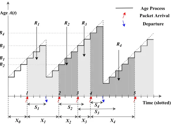
Time (slotted) X0 Age A(t) S1 Packet Arrival X1 X2 X3 S4 Departure S2 S3 2 3 4 1 A(t) Acont.(t) 1 1
Figure 2-1: Age 𝐴(𝑡) evolution over time 𝑡 along with the corresponding continuous age process. 𝑋𝑖 are inter-arrival times, 𝑆𝑖 are service times for packet 𝑖.
𝐴avecont. , lim sup
𝑇 →∞ 1 𝑇 ∫︁ 𝑇 𝑡=1 𝐴cont.(𝑡). (2.4)
We now relate the expressions of peak and average age in the discrete time sce-nario to the corresponding continuous time scesce-nario.
Theorem 1. The peak and average age for any discrete time queue, assuming that the peak and average age of the corresponding continuous time age process
are well defined, is given by
𝐴p= 𝐴pcont.− 1, (2.5)
and
𝐴ave = 𝐴avecont.− 1
2. (2.6)
Proof. An explanation for this result is easy to see via a graphical argument. Observe in Figure 2-1 that the peaks of 𝐴(𝑡) and 𝐴cont.(𝑡) always differ by 1. This is true
regardless of the service or arrival time distributions and the queuing discipline. Thus if the value 𝐴pcont. is well defined, 𝐴p is also well defined and is given by Equation 2.5.
Similarly, consider any time interval [𝑡, 𝑡 + 1). The discrete age process stays constant in this time interval at 𝐴(𝑡) and the area under the curve is just 𝐴(𝑡). The continuous age process 𝐴cont.(𝑡) increases from 𝐴(𝑡) to 𝐴(𝑡) + 1 in any such interval,
and the area under it is given by 𝐴(𝑡) + 12 since it has an added triangle of area 12. This implies that
∫︁ 𝑇 +1 𝑡=1 𝐴cont.(𝑡) = 𝑇 ∑︁ 𝑡=1 ∫︁ 𝑡+1 𝑡 𝐴cont.(𝑡) = 𝑇 ∑︁ 𝑡=1 (𝐴(𝑡) +1 2). (2.7)
Assuming that the continuous time average age 𝐴ave
cont. is well defined, we can
divide Equation 2.7 by 𝑇 + 1 and take the limit supremum as 𝑇 goes to ∞ to get Equation 2.6. This completes our proof.
Theorem 1 tells us that for the analysis for AoI in discrete time queues, it is sufficient to analyze the AoI of a corresponding continuous time queuing system with the same service and arrival distributions, and the same queuing discipline. As
discussed in Section 1.3, analysis for continuous time queuing systems has already been done in a variety of settings and can thus be directly applied to the discrete time setting. We discuss closed form expressions for AoI in a few discrete time systems in the following sections.
2.2
Geo/G/1 Queue
Consider a discrete time Geo/G/1 queue, where an arrival occurs at time 𝑡 with probability 𝜆 in an i.i.d. fashion, while the service times 𝑆 are generally distributed with mean E [𝑆] = 1/𝜇. The arrival process is thus i.i.d. geometric with parameter 𝜆, and both the arrival interval as well as service times are positive integers. According to our convention, if the service time of a packet is 1, then it gets served in the same time-slot as the one in which it was generated.
We obtain expressions for peak and average age for this discrete time Geo/G/1 queue. Observe that this corresponds to the FCFS G/G/1 setting analyzed in [25], but with the same arrival time distribution (i.i.d. geometric) and service time dis-tribution, albeit with support on positive integers.
Theorem 2. The peak and average age for the discrete time Geo/G/1 queue are given by 𝐴p= 1 𝜆 + 1 𝜇 + 𝜆E[𝑆2] − 𝜌 2(1 − 𝜌) − 1, (2.8) and 𝐴ave = 1 𝜇+ (1 − 𝜆)(1 − 𝜌) 𝜆𝐿𝑆(1 − 𝜆) +𝜆E[𝑆 2] − 𝜌 2(1 − 𝜌) , (2.9)
Proof. Using Theorem 1, we can use the expression for peak age derived for the corresponding continuous time FCFS queue from [25]
𝐴p = 𝐴pcont.− 1 = E [𝑇 + 𝑋] − 1, (2.10)
where 𝑇 denotes the time an update sends in the queue and 𝑋 is the inter-arrival time between two updates. From [58, Chapter 4.6.1], for a Geo/G/1 queue we have
E[𝑇 ] = 𝜆E[𝑆
2] − 𝜌
2(1 − 𝜌) + 1
𝜇, (2.11)
where 𝑆 denotes the service time. Substituting this and E [𝑋] = 1𝜆 in (2.10), we
obtain the expression for peak age.
For average age, we again find the average age of the corresponding continuous time system 𝐴ave
cont., and then use Theorem 1 to get the final result. For the derivation
of 𝐴avecont. see Appendix A.1.
We observe that the peak age expression for a Geo/G/1 queue is near identical to that of the M/G/1 queue derived in [26] with an additional term 2(1−𝜌)−𝜌 −1
2 added
due to the discretization. We use the probability generating function for analyzing average age due to the discrete nature of the service distribution.
2.3
Geo/G/1 Queue with Vacations
Consider a discrete time Geo/G/1 queue with vacations, where an arrival occurs at time 𝑡 with probability 𝜆 in an i.i.d. fashion, while the service times 𝑆 are generally distributed positive integers with mean E [𝑆] = 1/𝜇. When the queue is empty, the server takes i.i.d. vacations 𝑉 that are generally distributed with mean E [𝑉 ], until
a new arrival enters the queue. Geo/G/1 queues with vacations were used to find age optimal random walks for information dissemination on graphs in [27]. M/M/1 queues with vacations were also used to study the age of updates in a simple relay network in [59]. We obtain an expression for peak age and bounds for average age in the FCFS discrete time Geo/G/1 queue with vacations. Since the arrivals in any time time-slot are i.i.d. Bernoulli, from now on we refer to this queue as a Ber/G/1 queue with vacations.
Theorem 3. The peak age for the discrete time Ber/G/1 queue with vacations is given by 𝐴p= 1 𝜆 + 1 𝜇+ 𝜆E[𝑆2] − 𝜌 2(1 − 𝜌) + E [𝑉2] 2E [𝑉 ]− 3 2, (2.12)
and the average age is upper bounded by the peak age
𝐴ave ≤ 𝐴p+1
2. (2.13)
Proof. As usual, the peak age for the corresponding continuous time FCFS queue is given by [25]
𝐴pcont. = E [𝑇 + 𝑋] . (2.14)
Given that vacation times are distributed i.i.d according to random variable 𝑉 , using a residual time argument one can show that [60]
E[𝑇 ] = 𝜆E[𝑆 2] − 𝜌 2(1 − 𝜌) + 1 𝜇 + E [𝑉2] 2E [𝑉 ]− 1 2, (2.15)
Sub-stituting this and E [𝑋] = 𝜆1 in (2.14), we obtain the expression for peak age using
Theorem 1.
For the corresponding continuous time FCFS queue, the average age 𝐴ave cont. is
given by [1]
𝐴avecont. = E[𝑋
2 𝑛]/2 + E[𝑋𝑛𝑇𝑛] E[𝑋𝑛] = 1 𝜆 − 1 2 + 𝜆E[𝑋𝑛𝑇𝑛], (2.16) where 1𝜆 = E[𝑋𝑛] and a packet arrives in every time-slot with probability 𝜆, 𝑋1, 𝑋2, ...
are i.i.d. packet inter-arrival times and 𝑇1, 𝑇2, ... are corresponding times spent in the
system by each packet. Observe that 𝑋𝑛and 𝑇𝑛are negatively correlated (see [25] for
a proof). Intuitively, a smaller inter-arrival time means more congestion and more time spent in the system. Thus,
𝐴ave≤ 1 𝜆 − 1 2+ 𝜆E [𝑋𝑛] E [𝑇𝑛] = E [𝑋𝑛] + E [𝑇𝑛] − 1 2 = 𝐴 p +1 2, (2.17) where the last equality is due to Theorem 1. Thus, the average age is upper bounded by the peak age of the system up to a constant.
We observe that the peak age for a Ber/G/1 queue with vacations splits into two terms - the peak age for a Ber/G/1 queue without vacations, as derived in the previous section, and a term that depends only on the vacations. From Figure 2-2, we also observe numerically that the lighter the tail of the vacation distribution, better the age. We see that deterministic vacations minimize average age, given a fixed value of E [𝑉 ].
1 2 3 4 5 6 7 0 10 20 30 40 50 E[V] Average Age
Average Age − Ber/G/1 queue with vacations Geometric
Uniform Deterministic
Figure 2-2: Average age for geometrically distributed server times with probability 𝜇 = 0.75. We compare vacations with geometric, uniform bounded, and deterministic distributions having the same mean as it varies from 1 to 7. Solid lines represent arrival probability 𝜆 = 0.3 and dashed lines represent 𝜆 = 0.6.
Time (slotted) Age Process X0 B1 B3 Age A(t) S1 Packet Arrival X1 X2 X3 S4 Departure S2 X4 B2 B4 S3 R1 R2 R3 R4 1 2 3 4 5
Figure 2-3: Age 𝐴(𝑡) evolution in time 𝑡 for an LCFS queue with preemption.
2.4
LCFS Queues
Consider a discrete time LCFS G/G/1 queue with preemptive service, in which a newly arrived packet gets priority for service immediately. We assume that packets arrive at the beginning of a time-slot and leave at the end of a time-slot. Update packets are generated according to a renewal process, with inter-generation times distributed according to 𝑝𝑋. The service times are distributed according to 𝑝𝑆, i.i.d.
across packets.
Using Theorem 1 and results from [26], we can directly obtain closed form ex-pressions for peak and average age for general inter-generation and service time distributions.
Let 𝑋𝑖 denote the inter-generation time between the 𝑖th and (𝑖 + 1)th update
packet. Due to preemption, not all packets get serviced on time to contribute to age reduction. We illustrate this in Figure 2-3. Observe that packets 2 and 3 arrive before packet 4. However, packet 2 is preempted by packet 3, which is subsequently preempted by packet 4. Thus, packet 4 is serviced before 2 and 3. Service of packet 2 and 3 (not shown in figure) does not contribute to age curve 𝐴(𝑡) because they contain stale information.
Theorem 4. For the discrete time LCFS G/G/1 queue, the peak and average age are given by
𝐴pG/G/1= E [𝑋] P [𝑆 ≤ 𝑋] + E [𝑆I𝑆≤𝑋] P [𝑆 ≤ 𝑋] − 1, and 𝐴aveG/G/1= 1 2 E [𝑋2] E [𝑋] + E [min (𝑋, 𝑆)] P [𝑆 ≤ 𝑋] − 1 2,
where 𝑋 and 𝑆 denotes the independent inter-generation and service time random variables, respectively.
Proof. The proof follows directly from Theorem 1 and the age analysis of continuous time LCFS G/G/1 queues in [26]. For a more direct proof of this result, see [61].
Chapter 3
Mobility on a Graph
3.1
System Model
We consider a central terminal that needs to communicate with a set of ground terminals 𝑉 . The ground terminals are equipped with low power, low range radio communication devices, and cannot directly communicate with the central terminal, or with each other. An autonomous mobile agent 𝑚, is used as a relay between the central terminal and the ground terminals, while moving across the geographical region where the ground terminals are spread.
The mobility of the agent is constrained by a mobility graph 𝐺 = (𝑉, 𝐸), where 𝑚 can travel from ground terminal 𝑖 to ground terminal 𝑗 only if (𝑖, 𝑗) ∈ 𝐸. The graph 𝐺, thus, constraints the set of allowable moves. We consider a time-slotted system, with slot duration normalized to unity. In the duration of a time-slot, the mobile agent stays at a ground terminal to gather or disseminate information, and moves to any of its neighbours in 𝐺 for the next time-slot. The mobility graph can be constructed from the limitations of a slot duration, distances between ground
1 2 3 4 5 6 7 Ground Terminal Base Station Mobile Agent
terminals, and speed of the mobile agent.
We consider two problems: information gathering and information dissemination. In the information gathering problem, every time the mobile agent reaches a ground terminal 𝑖 ∈ 𝑉 , the ground terminal sends a fresh update to the mobile agent, which is immediately relayed to the central terminal. The age 𝐴𝑖(𝑡), at the central terminal,
for the ground terminal 𝑖 drops to 1. When the mobile agent is not at the ground terminal 𝑖, the age 𝐴𝑖(𝑡) increases linearly. See Figure 3-1. The evolution of 𝐴𝑖(𝑡) in
the information gathering problem can be written as:
𝐴𝑖(𝑡 + 1) = ⎧ ⎪ ⎨ ⎪ ⎩ 𝐴𝑖(𝑡) + 1, if 𝑚(𝑡) ̸= 𝑖 1, if 𝑚(𝑡) = 𝑖 (3.1)
where 𝑚(𝑡) denotes the location of the mobile agent at time 𝑡. Note that the age evolution depends on the trajectory that the mobile agent follows on the mobility graph 𝐺.
Time (slotted) Age Process H1,i H3,i 1 H1,i H3,i H2,i Agent m visits ground terminal i Age Ai(t)
Figure 3-1: Information gathering problem: time evolution of age 𝐴𝑖(𝑡); 𝐻𝑘,𝑖 is the
𝑘th return time to terminal 𝑖.
In the information dissemination problem, the central terminal generates updates for each ground terminal. The generated updates are then transmitted to the mobile agent. The mobile agent queues updates received from the central terminal in a set of 𝑉 FCFS queues, one for each ground terminal. The mobile agent delivers the head-of-line update in queue 𝑖, to ground terminal 𝑖, when it reaches 𝑖. The central terminal has no control over the FCFS queues on the mobile agent, however, it can control the update generation rate 𝜆𝑖, for each ground terminal 𝑖.
The age 𝐴𝑖(𝑡), at the ground terminal 𝑖, increases by 1 every time the mobile
agent is not at 𝑖, or when it is at 𝑖 but has no updates to deliver. Otherwise, a successful delivery of the head-of-line update occurs in time slot 𝑡, and the age 𝐴𝑖(𝑡)
t1' Age Ai(t) Time (slotted) Age Process t1 t2 t2' t3 t3' t4 t4' t1' t1 + 1 Agent m visits ground terminal i and Qi(t) is not empty t3' t3 + 1
Figure 3-2: Information dissemination problem: time evolution of age 𝐴𝑖(𝑡); 𝑡𝑘, 𝑡′𝑘
are the generation and reception times of the 𝑘th status update for terminal 𝑖.
of age 𝐴𝑖(𝑡) can be written as:
𝐴𝑖(𝑡 + 1) = ⎧ ⎪ ⎪ ⎪ ⎪ ⎪ ⎨ ⎪ ⎪ ⎪ ⎪ ⎪ ⎩ 𝐴𝑖(𝑡) + 1, if 𝑚(𝑡) ̸= 𝑖 𝐴𝑖(𝑡) + 1, if 𝑚(𝑡) = 𝑖 and 𝒬𝑖(𝑡) = ∅ 𝑡 − 𝐺𝑖(𝑡) + 1, if 𝑚(𝑡) = 𝑖 and 𝒬𝑖(𝑡) ̸= ∅ , (3.2)
where 𝐺𝑖(𝑡) is the time of generation of the head of line packet in queue 𝑖, at time 𝑡,
and 𝒬𝑖(𝑡) denotes the set of packets in the mobile agent’s queue 𝑖 at time 𝑡.
3.1.1
Age Metrics
AoI is an evolving function of time. We consider two time average metrics of AoI. Average age, for ground terminal 𝑖, is defined as the time averaged area under the
age curve:
𝐴ave𝑖 , lim sup
𝑇 →∞ 1 𝑇 𝑇 ∑︁ 𝑡=1 𝐴𝑖(𝑡). (3.3)
In Figures 3-1 and 3-2, we see that the age 𝐴𝑖(𝑡) peaks before a fresh update is
delivered. In the information gathering case, a fresh update is delivered every time the mobile agent visits 𝑖, i.e. 𝑚(𝑡) = 𝑖. Whereas, in the information dissemination case, a fresh update is delivered whenever 𝑚(𝑡) = 𝑖 and the queue 𝒬𝑖(𝑡) ̸= ∅. The
peak age 𝐴p𝑖, for ground terminal 𝑖, defined as an average of all the peaks in the age evolution curve 𝐴𝑖(𝑡), can be written as
𝐴p𝑖 , lim sup 𝑇 →∞ 𝑡=𝑇 ∑︀ 𝑡=1 𝐴𝑖(𝑡)1{𝑚(𝑡)=𝑖} 𝑡=𝑇 ∑︀ 𝑡=1 1{𝑚(𝑡)=𝑖} , (3.4)
in the information gathering case and
𝐴p𝑖 , lim sup 𝑇 →∞ 𝑡=𝑇 ∑︀ 𝑡=1 𝐴𝑖(𝑡)1{𝑚(𝑡)=𝑖,𝒬𝑖(𝑡)̸=∅} 𝑡=𝑇 ∑︀ 𝑡=1 1{𝑚(𝑡)=𝑖,𝒬𝑖(𝑡)̸=∅} , (3.5)
in the information dissemination case.
We define the network peak and average age to be
𝐴p =∑︁ 𝑖∈𝑉 𝑤𝑖𝐴p𝑖 and 𝐴 ave =∑︁ 𝑖∈𝑉 𝑤𝑖𝐴ave𝑖 , (3.6)
where 𝑤𝑖 > 0 are weights representing the relative importance of a ground terminal
3.1.2
Trajectory Space
We use T to denote a reasonably large space of trajectories:
T = { Trajectory 𝒯 | 𝑓𝑖(𝒯 ) exists and is positive ∀ 𝑖 ∈ 𝑉 } ,
where 𝑓𝑖(𝒯 ) denotes the fraction of time-slots, the trajectory 𝒯 , is at ground terminal
𝑖: 𝑓𝑖(𝒯 ) = lim 𝑇 →∞ 1 𝑇 𝑇 ∑︁ 𝑡=1 1{𝑚(𝑡)=𝑖}. (3.7)
For a trajectory 𝒯 ∈ T, the limit (3.7) exists and is positive for all 𝑖 ∈ 𝑉 . This requirement is to ensure that the peak and average age are both finite and well defined.
Peak and average age depend on the trajectory 𝒯 ∈ T. We use 𝐴p(𝒯 ) and
𝐴ave(𝒯 ) to denote network peak and average age, respectively, for 𝒯 ∈ T. In the
following two sections, we introduce the problem of finding trajectories that minimize network peak and average age, and try to find solutions to these problems.
3.2
Information Gathering
In this section, we consider the problem of age optimal information gathering with active sources. We define optimal peak and average age to be
𝐴p*𝒢 = min 𝒯 ∈T𝐴 p(𝒯 ), and 𝐴ave* 𝒢 = min 𝒯 ∈T𝐴 ave(𝒯 ), (3.8)
where T denotes the space of all trajectories for the mobile agent.
accord-ing to a random walk on the mobility graph. We shall show that for peak age optimality, such randomized trajectories suffices. We then show that the average age optimization is NP-hard, and propose a heuristic randomized trajectory. In Sec-tion 3.2.5, we propose an age-based trajectory for better average age performance.
3.2.1
Randomized Trajectories
We start by defining the class of randomized trajectories:
Definition A trajectory 𝑚(𝑡), on mobility graph 𝐺, is said to be a randomized trajectory if 𝑚(𝑡) is an irreducible Markov chain defined by a transition proba-bility matrix P:
P𝑚(𝑡 + 1) = 𝑗|𝑚(𝑡) = 𝑖 = 𝑃𝑖,𝑗, (3.9)
for all 𝑡 and 𝑖, 𝑗 ∈ 𝑉 , where 𝑃𝑖,𝑗 = 0 for (𝑖, 𝑗) /∈ 𝐸.
For convenience, we shall refer to 𝑚(𝑡), defined above, as the randomized tra-jectory P, where P to denote the matrix with entries 𝑃𝑖,𝑗. Note that 𝑃𝑖,𝑗 is the
probability that the mobile agent, when at ground terminal 𝑖, moves to ground ter-minal 𝑗 for the next time slot. The constraint: 𝑃𝑖,𝑗 = 0 for (𝑖, 𝑗) /∈ 𝐸, ensures that
the randomized trajectory adheres to the mobility constraints defined by 𝐺.
We assume in the definition of a randomized trajectory P, that 𝑚(𝑡) is an irre-ducible Markov chain over the state space 𝑉 . This is desired, since the mobile agent has to traverse through all the nodes, repeatedly, for a positive fraction of time, or otherwise the resulting peak and average age would be unbounded.
For any randomized trajectory P, we obtain explicit expressions for network peak and average age. We use the notation 𝐴p(P) and 𝐴ave(P) to show explicit dependence of peak and average age on the randomized trajectory P.
Theorem 5. The network peak and average age for a randomized trajectory P is given by 𝐴p(P) =∑︁ 𝑖∈𝑉 𝑤𝑖 𝜋𝑖 , and 𝐴ave(P) =∑︁ 𝑖∈𝑉 𝑤𝑖𝑧𝑖𝑖 𝜋𝑖 , (3.10)
where 𝜋 is the unique stationary distribution obtained by solving 𝜋P = 𝜋 and 𝑧𝑖𝑖
are diagonal elements of the matrix 𝑍 , (𝐼 − P + Π)−1, where Π is an 𝑛 × 𝑛 matrix with entries Π𝑖,𝑗 , 𝜋𝑗, ∀𝑖, 𝑗 ∈ 𝑉 .
Proof. The key step in proving the result above is to observe that the peak age of the ground terminal 𝑖, namely 𝐴p𝑖, depends only on the mean of return times to terminal 𝑖; see Figure 3-1. Whereas, the average age 𝐴ave
𝑖 for 𝑖 depends on both, the mean
and the variance, of return times to terminal 𝑖.
Given a randomized trajectory P, the mean of return times to terminal 𝑖 is given by 𝜋1
𝑖, while the second moment of the return times is given by −1
𝜋𝑖 + 2𝑧𝑖𝑖
𝜋2𝑖 ; see [62].
Using this fact, we are able to obtain the explicit expressions for peak and average age. Let 𝐴𝑝𝑖 be the peak age for ground terminal 𝑖. We define 𝐻𝑘,𝑖 to be the 𝑘th
return time to ground terminal 𝑖. Then, the 𝑘th age peak for 𝐴
𝑖(𝑡) has a value of
expected peak age of ground terminal 𝑖 is given by 𝐴𝑝𝑖 = lim 𝑇 →∞E [︃ 𝑡=𝑇 ∑︀ 𝑡=1 𝐴𝑖(𝑡)1{𝑚(𝑡)=𝑖} 𝑡=𝑇 ∑︀ 𝑡=1 1{𝑚(𝑡)=𝑖} ]︃ = lim 𝐾→∞E [︂ 1 𝐾 𝑡=𝐾 ∑︁ 𝑘=1 𝐻𝑘,𝑖 ]︂ . (3.11)
Note that return times to a ground terminal 𝑖 are i.i.d. random variables given a randomized trajectory P. So, we can use the law of large numbers to get
𝐴𝑝𝑖 = E[𝐻1,𝑖] =
1 𝜋𝑖
, (3.12)
where 𝜋𝑖 is the stationary distribution for Markov chain P. The last equality follows
from the fact that the expected return time to a state 𝑖 for an irreducible Markov chain is given by the inverse of its stationary probability. Thus, the network age is given by 𝐴p =∑︁ 𝑖∈𝑉 𝑤𝑖𝐴𝑝𝑖 = ∑︁ 𝑖∈𝑉 𝑤𝑖 𝜋𝑖 . (3.13)
For average age, we define a renewal-reward process using 𝐻𝑘,𝑖 as our i.i.d.
renewal intervals and sum of age 𝐴𝑖(𝑡) during each interval as our reward. Let
𝑇𝑘,𝑖 =
∑︀𝑘−1
𝑙=1 𝐻𝑙,𝑖 be the starting time of the 𝑘th renewal. The total reward in
be-tween two visits to ground terminal 𝑖 is the sum of the 𝑖th age process 𝐴𝑖(𝑡) across
all time-slots during that interval.
Note that, for the 𝑘th renewal interval, 𝐴𝑖(𝑡) grows from 1 to 𝐻𝑘,𝑖 over the 𝐻𝑘,𝑖
time-slots. Thus, the total reward for the 𝑘th renewal interval is given by -𝑡=𝑇𝑘,𝑖+𝐻𝑘,𝑖 ∑︁ 𝑡=𝑇𝑘,𝑖 𝐴𝑖(𝑡) = 𝐻𝑘,𝑖 ∑︁ 𝑎=1 𝑎 = 𝐻 2 𝑘,𝑖+ 𝐻𝑘,𝑖 2 . (3.14)
Note that this reward is also i.i.d. across renewals as it depends only on 𝐻𝑘,𝑖. Thus,
by application of the elementary renewal theorem for renewal-reward processes we get 𝐴ave𝑖 = lim 𝑇 →∞E [︂ 1 𝑇 𝑡=𝑇 ∑︁ 𝑡=1 𝐴𝑖(𝑡) ]︂ = E[𝐻 2 1,𝑖+ 𝐻1,𝑖] 2E[𝐻1,𝑖] . (3.15)
For irreducible Markov chains, we know the following results hold [62]:
E[𝐻1,𝑖] = 1 𝜋𝑖 , ∀𝑖 ∈ 𝑉 and (3.16) E[𝐻1,𝑖2 ] = −1 𝜋𝑖 + 2𝑧𝑖𝑖 𝜋2 𝑖 , (3.17)
for all 𝑖 ∈ 𝑉 , where 𝑧𝑖𝑖 is the 𝑖th diagonal element of the matrix 𝑍 = (𝐼 − 𝑃 + Π)−1,
with Π being a matrix in which all rows are the stationary distribution vector 𝜋: Π𝑖,𝑗 = 𝜋𝑗 for all 𝑖, 𝑗 ∈ 𝑉 .
Substituting (3.16) and (3.17) in (3.15), we get
𝐴ave𝑖 = 𝑧𝑖𝑖 𝜋𝑖
, (3.18)
for all 𝑖 ∈ 𝑉 , and therefore,
𝐴ave =∑︁ 𝑖∈𝑉 𝑤𝑖𝐴ave𝑖 = ∑︁ 𝑖∈𝑉 𝑤𝑖𝑧𝑖𝑖 𝜋𝑖 . (3.19)
3.2.2
Peak Age Minimization
We first formulate the peak age minimization problem over the space of randomized trajectories. We shall see that a peak age optimal randomized trajectory suffices for
optimality over the space of all trajectories.
Using the results in Theorem 5, we can write the peak age minimization problem over the space of randomized trajectories as:
Minimize P,𝜋 ∑︁ 𝑖∈𝑉 𝑤𝑖 𝜋𝑖 , subject to 𝑃𝑖,𝑗 ≥ 0, ∀(𝑖, 𝑗), and P1 = 1, 𝜋P = 𝜋, 1𝑇𝜋 = 1, and 𝜋𝑖 ≥ 0 ∀𝑖 𝑃𝑖,𝑗 = 0, ∀(𝑖, 𝑗) /∈ 𝐸, P is irreducible. (3.20)
Note that P characterizes a randomized trajectory, while 𝜋 is the unique stationary distribution associated with it.
This problem is difficult to solve because the irreducibility constraint cannot be expressed in a simple, solvable manner. Further, relaxing the irreducibility constraint can yield a trivial solution like P = 𝐼, which are neither irreducible nor anywhere close to optimal.
However, the problem (3.20) can be transformed to finding an irreducible P, with a given stationary distribution. This is a simpler problem and can be solved using the Metropolis-Hastings algorithm.
Lemma 1. Let 𝜋*𝑖 , √ 𝑤𝑖 ∑︀ 𝑗∈𝑉 √
𝑤𝑗, for all 𝑖 ∈ 𝑉 , to be a distribution on 𝑉 , and a
randomized trajectory P satisfy 𝜋*P = 𝜋*. Then, (𝜋*, P) solves (3.20).
Proof. Suppose we could choose any stationary distribution 𝜋 on 𝑉 . Then to mini-mize the network peak age, we would need to solve the following optimization
prob-lem Minimize 𝜋 ∑︁ 𝑖∈𝑉 𝑤𝑖 𝜋𝑖 , subject to ∑︁ 𝑖 𝜋𝑖 = 1, 𝜋𝑖 ≥ 0, ∀𝑖 ∈ 𝑉. (3.21)
Using KKT conditions for the optimization problem (3.21), it is straightforward to see that 𝜋𝑖* = √ 𝑤𝑖 ∑︀ 𝑖 √ 𝑤𝑖 , ∀𝑖 ∈ 𝑉. (3.22)
Clearly, if we could find a randomized trajectory P that achieves this stationary distribution 𝜋*, then it would be peak age optimal. Thus, any randomized trajectory P that satisfies 𝜋* = 𝜋*P is peak age optimal.
Observe that the expression above implies that the fraction of time spent at a node is proportional to the square root of its weight. This is similar to the “square root principle” first derived in peer-to-peer settings in [63]. Similar square root based scheduling results have been derived for minimizing age in single hop networks [18,64] Lemma 1 implies that a randomized trajectory P, that satisfies 𝜋*P = 𝜋*, is a peak age optimal, over the space of all randomized trajectories. We now construct one such randomized trajectory: for 𝜋* given in Lemma 1, define a Metropolis-Hastings randomized trajectory Pmh: 𝑃𝑖,𝑗mh = ⎧ ⎪ ⎪ ⎪ ⎪ ⎪ ⎨ ⎪ ⎪ ⎪ ⎪ ⎪ ⎩ 𝑃𝑖,𝑗rwmin(1,𝜋 * 𝑗𝑃𝑗,𝑖rw 𝜋*𝑖𝑃rw 𝑖,𝑗), if 𝑖 ̸= 𝑗 and (𝑖, 𝑗) ∈ 𝐸 1 − ∑︀ 𝑗:𝑗̸=𝑖 𝑃𝑖,𝑗mh, if 𝑖 = 𝑗 0, otherwise , (3.23)
where 𝑃𝑖,𝑗rw = ⎧ ⎪ ⎨ ⎪ ⎩ 1 𝑑𝑖, if 𝑖 ̸= 𝑗 and (𝑖, 𝑗) ∈ 𝐸 0, otherwise , ∀𝑖, 𝑗 ∈ 𝑉, (3.24)
and 𝑑𝑖 equals the out degree of terminal 𝑖 in the mobility graph 𝐺. It is known that
such a randomized trajectory Pmh satisfies 𝜋*P = 𝜋* [62]. We, therefore, have the following result.
Theorem 6. The Metropolis-Hastings randomized trajectory Pmh solves (3.20),
i.e. it is peak age optimal over the space of all randomized trajectories.
We considered randomized trajectories, where the mobile agent moves from ter-minal 𝑖 to 𝑗 with probability 𝑃𝑖,𝑗. We now show that, for peak age optimality, such
a randomization suffices.
Theorem 7. The Metropolis-Hastings randomized trajectory Pmh is peak age
optimal over the space of all trajectories T, namely 𝐴p*(Pmh) = 𝐴p* 𝒢 .
Proof. We establish a more general result. Namely, any randomized trajectory which satisfies 𝜋*P = 𝜋*, where 𝜋𝑖* = √ 𝑤𝑖 ∑︀ 𝑗∈𝑉 √
𝑤𝑗, is peak age optimal over the space of all
trajectories:
𝐴p*(P) = 𝐴p*𝒢 .
To prove this, it suffices to argue that the peak age for any trajectory is lower bounded by∑︀ 𝑖∈𝑉 𝑤𝑖 𝜋* 𝑖, where 𝜋 * is as given in Theorem 6.
Let 𝐻𝑘,𝑖 to be the 𝑘th return time to node 𝑖. If 𝐾 is the total number of returns
to ground terminal 𝑖 over a time horizon 𝑇 , then the peak age 𝐴p𝑖 is given by
𝐴p𝑖 = lim sup 𝑇 →∞ 𝑡=𝑇 ∑︀ 𝑡=1 𝐴𝑖(𝑡)1{𝑚(𝑡)=𝑖} 𝑡=𝑇 ∑︀ 𝑡=1 1{𝑚(𝑡)=𝑖} = lim sup 𝐾→∞ 1 𝐾 𝑘=𝐾 ∑︁ 𝑘=1 𝐻𝑘,𝑖. (3.25)
Now, the fraction of time-slots in which the mobile agent is at ground terminal 𝑖, is given by 𝑓𝑖 = lim 𝑇 →∞ 𝑡=𝑇 ∑︀ 𝑡=1 1{𝑚(𝑡)=𝑖} 𝑇 = lim𝐾→∞ 𝐾 𝑘=𝐾 ∑︀ 𝑘=1 𝐻𝑘,𝑖 = 1 𝐴p𝑖, (3.26) and therefore, 𝐴p = ∑︀ 𝑖∈𝑉 𝑤𝑖𝐴 p 𝑖 = ∑︀ 𝑖∈𝑉 𝑤𝑖
𝑓𝑖. Note that 𝑓𝑖, being the fraction of
time-slots the mobile agent is at terminal 𝑖, is a distribution over 𝑉 . Thus, 𝐴p can
be lower bounded by 𝐴p =∑︁ 𝑖∈𝑉 𝑤𝑖𝐴 𝑝 𝑖 ≥ min {𝑓𝑖≥0, ∑︀𝑖𝑓𝑖=1} ∑︁ 𝑖∈𝑉 𝑤𝑖 𝑓𝑖 =∑︁ 𝑖∈𝑉 𝑤𝑖 𝜋𝑖*, (3.27)
where the last equality is obtained by solving the optimization problem, just as in the proof of Lemma 1.
Thus, we are able to obtain a peak age optimal trajectory, namely Pmh. Further, the matrix Pmh can be computed in polynomial time; in 𝑂(|𝑉 |2) time. Therefore,
the peak age minimization problem is solved in polynomial time. For details on how to derive the Metropolis-Hastings Markov chain and a nice geometric interpretation, see [65] and [66].
3.2.3
Average Age Minimization
We now consider the average age minimization problem. We first argue that in the symmetric setting, namely 𝑤𝑖 = 1 ∀ 𝑖 ∈ 𝑉 ,1 the average age minimization problem
is NP-hard
Theorem 8. The problem of finding an average age optimal trajectory is NP-hard in the symmetric setting of 𝑤𝑖 = 1 ∀ 𝑖 ∈ 𝑉 .
Proof. To prove NP-hardness, we establish equivalence between the average age min-imization problem and the Hamiltonian cycle problem, in the symmetric setting. We know that more connected the graph, lower is its network average age. Therefore, the average age for G = (V, E) is lower bounded by the average age for the com-plete graph K(V), given by |𝑉 |(|𝑉 |+1)2 . This lower bound can be obtained by using Theorem 9 and setting 𝑤𝑖 = 1, ∀𝑖.
If the graph is Hamiltonian, we can achieve this average age lower bound by setting the trajectory equal to a Hamiltonian cycle. This is because in a cyclical trajectory, the agent visits every terminal exactly once in every |𝑉 | time-slots. Fur-ther, if the graph is not Hamiltonian, the optimal average age is strictly greater than
|𝑉 |(|𝑉 |+1)
2 . This is because in the absence of a cycle on graph 𝐺, the agent cannot visit
every terminal exactly once every |𝑉 | time-slots. Therefore, if an algorithm were to solve the average age problem then the same algorithm could be used to determine whether the graph G is Hamiltonian or not; which is the Hamiltonian cycle problem. Since the Hamiltonian cycle problem is NP-complete, the average age minimization
1The weights 𝑤
𝑖 only measure relative significance of ground terminals. Thus, setting 𝑤𝑖 =
problem must be NP-hard.
Since solving the average age minimization problem is hard, we derive a lower bound on average age. Intuitively, if the mobility graph is better connected then it should yield a lower age. This is because a better connected mobility graph imposes fewer restrictions on mobility. The following result obtains a lower bound on network average age by comparing it with the network average age of a complete graph.
Theorem 9. For any trajectory 𝒯 ∈ T, the network average age is lower bounded by 𝐴ave(𝒯 ) ≥ 1 2 ∑︁ 𝑖∈𝑉 (︂ 𝑤𝑖 𝜋𝑖* + 𝑤𝑖 )︂ , (3.28) where 𝜋𝑖* = √ 𝑤𝑖 ∑︀ 𝑗∈𝑉 √ 𝑤𝑗 for all 𝑖 ∈ 𝑉 .
Proof. Let 𝐻𝑘,𝑖 be the 𝑘th return time to ground terminal 𝑖, and 𝐾 be the total
number of returns to 𝑖 over a time-horizon 𝑇 . Then the average age 𝐴ave
𝑖 is given by
(see proof of Theorem 1):
𝐴ave𝑖 = lim 𝑇 →∞ 1 𝑇 𝑡=𝑇 ∑︁ 𝑡=1 𝐴𝑖(𝑡) = lim 𝐾→∞ 𝑘=𝐾 ∑︀ 𝑘=1 (𝐻𝑘,𝑖2 + 𝐻𝑘,𝑖) 2 𝑘=𝐾 ∑︀ 𝑘=1 𝐻𝑘,𝑖 . (3.29)
Define the empirical first and second moment of return times be ˆ𝐻𝑖 , 𝐾1 𝑘=𝐾 ∑︀ 𝑘=1 𝐻𝑘,𝑖 and ˆ𝐻𝑖(2) , 𝐾1 𝑘=𝐾 ∑︀ 𝑘=1
𝐻𝑘,𝑖2 , respectively. Further, define Varˆ 𝑖 , ˆ𝐻 (2)
empirical variance of return times. From (3.29), we have 𝐴ave𝑖 = 1 2 + lim𝐾→∞ ˆ 𝐻𝑖(2) 2 ˆ𝐻𝑖 = 1 2 + lim𝐾→∞ (︁ ˆ𝐻𝑖)︁2 + ˆVar𝑖 2 ˆ𝐻𝑖 . (3.30)
Using Cauchy-Schwarz inequality, we can obtain ˆVar𝑖 ≥ 0. Applying this to (3.30),
we get 𝐴ave𝑖 ≥ 1 2+ lim𝐾→∞ ˆ 𝐻𝑖 2 , (3.31)
Let 𝑓𝑖 be the fraction of time-slots in which the mobile agent is at ground terminal
𝑖. Then, 𝑓𝑖 = lim 𝑇 →∞ 𝑡=𝑇 ∑︀ 𝑡=1 1{𝑚(𝑡)=𝑖} 𝑇 = lim𝐾→∞ 𝐾 𝑘=𝐾 ∑︀ 𝑘=1 𝐻𝑘,𝑖 = 1 lim𝐾→∞𝐻ˆ𝑖 , (3.32)
since 𝑓𝑖 is well defined and positive for all trajectories in T. Substituting (3.32)
in (3.31) we get 𝐴ave
𝑖 ≥
1 2 +
1
2𝑓𝑖, for all 𝑖, and
𝐴ave =∑︁ 𝑖∈𝑉 𝑤𝑖𝐴ave𝑖 ≥ 1 2 ∑︁ 𝑖∈𝑉 𝑤𝑖+ 1 2 ∑︁ 𝑖∈𝑉 𝑤𝑖 𝑓𝑖 . (3.33)
Note that 𝑓𝑖, being the fraction of time-slots the mobile agent is at terminal 𝑖, is a
distribution over 𝑉 . Thus, the average age in (3.33) can be lower bounded by
𝐴ave≥ 1 2 ∑︁ 𝑖∈𝑉 𝑤𝑖+ 1 2{𝑓𝑖≥0,min∑︀𝑖𝑓𝑖=1} ∑︁ 𝑖∈𝑉 𝑤𝑖 𝑓𝑖 , = 1 2 ∑︁ 𝑖∈𝑉 𝑤𝑖+ 1 2 ∑︁ 𝑖∈𝑉 𝑤𝑖 𝜋𝑖*,
Note that the term ∑︀
𝑖∈𝑉 𝑤𝑖 𝜋*
𝑖 is nothing but the optimal peak age 𝐴 p*
𝒢 ; see
Theo-rem 7. Furthermore, the lower bound in TheoTheo-rem 9 is independent of the trajectory 𝒯 . Therefore, we get 𝐴ave*𝒢 = min 𝒯 ∈T𝐴 ave(𝒯 ) ≥ 𝐴ave LB = 1 2𝐴 p* 𝒢 + 1 2 ∑︁ 𝑖∈𝑉 𝑤𝑖, (3.34)
where T is the space of all trajectories. It must be noted that a similar result was derived in the case of link scheduling for age minimization in [15]. The similarity of the result is rooted in the fact that the information gathering problem in the complete graph case is equivalent to the link scheduling problem in [15], in which at most one link can be activated simultaneously.
3.2.4
A Heuristic Randomized Trajectory
Motivated by the peak age optimality results of the previous section, we restrict ourselves to the space of randomized trajectories, and propose a heuristic, called the fastest-mixing randomized trajectory, and prove an average age performance bound for it.
space of randomized trajectories can be written as Minimize P,𝜋,Z ∑︁ 𝑖∈𝑉 𝑤𝑖𝑧𝑖𝑖 𝜋𝑖 , subject to 𝑃𝑖,𝑗 ≥ 0, ∀ (𝑖, 𝑗), and P1 = 1, 𝜋P = 𝜋, 1𝑇𝜋 = 1, and 𝜋𝑖 ≥ 0 ∀𝑖 𝑃𝑖,𝑗 = 0, ∀(𝑖, 𝑗) /∈ 𝐸, P is irreducible, Π𝑖,𝑗 = 𝜋𝑗 ∀ (𝑖, 𝑗), 𝑍 = (𝐼 − P + Π)−1. (3.35)
Here, P is the randomized trajectory and 𝜋 the unique stationary distribution corre-sponding to P. Solving (3.35) can be computationally complex. Not only do we have the irreducibility constraint, but also a non-linear constraint in 𝑍 = (𝐼 − P + Π)−1. We next upper bound the network average age, for any randomized trajectory P of the mobile agent. We first define mixing time for a randomized trajectory.
To do this, we first discuss the notion of stopping rules and stopping times in a Markov chain. A stopping rule is a rule that observes the walk on a Markov chain and, at each step, decides whether or not to stop the walk based on the walk so far. Stopping rules can make probabilistic decisions and therefore the time at which the walk stops, called the stopping time, is a random variable.
Mixing Time [67] The hitting time from state distribution 𝜎1 to 𝜎2 on a Markov
chain is the minimum expected stopping time over all stopping rules that, beginning at 𝜎1, stop in the exact distribution of 𝜎2. In other words, it is the expected number
by ℋ(𝜎1, 𝜎2). The mixing time ℋ of a Markov chain P is then defined as
ℋ , sup
𝜎∈Δ(𝑉 )
ℋ(𝜎, 𝜋), (3.36)
where Δ(𝑉 ) is the collection of all distributions on 𝑉 and 𝜋 is the stationary distri-bution of P. In other words, it is the expected time taken to reach stationarity using the optimal stopping rule and starting at the worst initial distribution.
Lemma 2. The network average age for a randomized trajectory P is upper bounded by 𝐴ave(P) =∑︁ 𝑖∈𝑉 𝑤𝑖𝑧𝑖𝑖 𝜋𝑖 ≤ 4ℋ𝐴p(P) +∑︁ 𝑖∈𝑉 𝑤𝑖, (3.37)
where ℋ denotes the mixing time of the randomized trajectory P.
Proof. First, we define the quantity
𝒵 , max
𝑖
∑︀
𝑗
|𝑧𝑖𝑗 − 𝜋𝑗|, called the discrepancy of the randomized trajectory P. This
definition implies that 𝑧𝑖𝑖 ≤ 𝒵 + 𝜋𝑖, ∀𝑖 ∈ 𝑉. Thus, we get the following upper bound:
∑︁ 𝑖∈𝑉 𝑤𝑖𝑧𝑖𝑖 𝜋𝑖 ≤∑︁ 𝑖∈𝑉 (︂ 𝑤𝑖𝒵 𝜋𝑖 + 𝑤𝑖 )︂ . (3.38)
However, from [68] we know that 𝒵 ≤ 4ℋ, where ℋ is the mixing time of the randomized trajectory P. Thus, we have the required result
∑︁ 𝑖∈𝑉 𝑤𝑖𝑧𝑖𝑖 𝜋𝑖 ≤∑︁ 𝑖∈𝑉 (︂ 4𝑤𝑖ℋ 𝜋𝑖 + 𝑤𝑖 )︂ = 4ℋ𝐴p(P) +∑︁ 𝑖∈𝑉 𝑤𝑖,
We use this relation and suggest the following heuristic for minimizing age: Find the fastest mixing randomized trajectory P on the mobility graph 𝐺 that minimizes peak age.
From the proof of Theorem 7, we know that for a randomized trajectory P to be peak age optimal all we need is 𝜋𝑖 ∝
√
𝑤𝑖, where 𝜋 is the stationary distribution
of P. It, therefore, suffices to find P that satisfies 𝜋𝑖 ∝
√
𝑤𝑖, and simultaneously
minimizes the mixing time ℋ. We call this the fastest-mixing randomized trajectory, and use P* to denote it. The following result provides a way to obtain P* by solving a convex program.
Theorem 10. The fastest mixing randomized trajectory can be found by solving the following convex optimization problem:
Minimize P 𝜇(P) = ||P − Π *|| 2, subject to 𝑃𝑖,𝑗 ≥ 0, ∀(𝑖, 𝑗), P1 = 1, 𝜋*P = 𝜋*, Π*𝑖,𝑗 = 𝜋*𝑖 ∀ 𝑖, 𝑗 ∈ 𝑉, 𝑃𝑖,𝑗 = 0, ∀(𝑖, 𝑗) /∈ 𝐸. (3.39)
Here ||𝐴||2 denotes the spectral norm of matrix 𝐴 and 𝜋𝑖* = √ 𝑤𝑖 ∑︀ 𝑗∈𝑉 √ 𝑤𝑗, ∀𝑖 ∈ 𝑉 .
Proof. From [65], we know that the fastest mixing, reversible Markov chain on a graph 𝐺(𝑉, 𝐸) having the stationary distribution 𝜋 can be found by formulating the