AEROELASTIC PROPERTIES OF STRAIGHT AND FORWARD SWEPT GRAPHITE/EPOXY WINGS
by
BRIAN JEROME LANDSBERGER
B.S., United States Air Force Academy (1972)
SUBMITTED TO THE DEPARTMENT OF AERONAUTICS AND ASTRONAUTICS IN PARTIAL
FULFILLMENT OF THE REQUIREMENTS FOR THE DEGREE OF
MASTER OF SCIENCE IN
AERONAUTICS AND ASTRONAUTICS at the
MASSACHUSETTS INSTITUTE OF TECHNOLOGY
February, 1983
Massachusetts Institute of Technology 1983
Signature of Author
Department of Aeronautics nd'Astronautics
December 14, 1982 Certified by John 'Duqundji' Thesis Supervisor Accepted by i i Harold Y. Wachman
ArchiveSChairman,
Departmental Graduate Comittee MASSACHUSETTS INSTITUTEOF TECHNOLOGY
MAR
3
0
1983
AEROELASTIC PROPERTIES OF STRAIGHT AND FORWARD SWEPT GRAPHITE/EPOXY WINGS
by
BRIAN JEROME LANDSBERGER
Submitted to the Department of Aeronautics and Astronautics on December 14, 1982, in partial fulfillment of the requirements for the degree of
Master of Science in Aeronautics and Astronautics.
ABSTRACT
The aeroelastic deformation, divergence and flutter behavior of rectangular, graphite/epoxy, cantilevered plate type wings at zero sweep and thirty degrees of forward sweep is investigated for incompressible flow. Since the wings have varying amounts of bending stiffness, torsion stiffness and bending-torsion stiffness coupling, they each have unique aeroelastic properties. A five mode Rayleigh-Ritz formulation is used to calculate the equation of motion. From this equation static deflection, steady airload deflection, divergence velocities, natural frequencies and flutter velocities are calculated. Experimental two dimensional lift and drag curve data and approximations to three dimensional aerodynamics are used to calculate the aerodynamic forces for the steady airload analysis. The Weissinger L-Method for three dimensional aerodynamic forces is used in the divergence analysis. The V-g method is used to make flutter and natural frequency calculations. Tests on a static loading apparatus gave static deflections, while wind tunnel tests gave steady airload deflections for the wings at zero sweep, and divergence
and flutter behavior data for all wings at both zero sweep and thirty
degrees forward sweep. Wings were tested from zero to twenty degrees angle of attack for airspeeds up to divergence, flutter or the thirty
meter per second limit of the tunnel.
Static deflection, natural frequencies, steady airload, divergence
and flutter for the straight wing were predicted reasonably well by the
theoretical calculations. For the swept forward wings, calculated flutter speeds were beyond the wind tunnel capabilities, while calculated divergence speeds were reasonable when divergence did occur. When swept forward, before reaching predicted divergence speeds some lightly bending-torsion stiffness coupled wings went into a torsional flutter, characterized by a large average bend which caused a high wing tip angle of attack. This flutter was not predicted by the theory used. The different ' wings exhibited markedly different stall flutter
characteristics.
Thesis Supervisor: John Dugundji Title: Professor of Aeronautics and Astronautics
ACKNOWLEDGEMENTS
I thank Professor John Dugundji for his continuous guidance during all phases of this project. I also thank Rob Dare, a fellow student, who assisted me during all experimental work.
Finally, to all the staff of M.I.T. who's instruction and assistance made this project possible, and to the United States Air Force
which funded my education and the contract covering this project, a
TABLE OF CONTENTS Page List of Figures...6 List of Tables...7 List of Symbols...8 Chapter 1. Introduction... 11 2. Theory 2.1 2.2 2.3 2.4 2.5 Rayleigh-Ritz Analysis...12
Static Deflection Analysis...23
Steady Airload Analysis...25
Divergence Analysis... .... 34
Flutter Analysis... ... 44
3. Experiments 3.1 Test Wing Selection... 3.2 Static Deflection Tests ... 3.3 Wind Tunnel Test Setup... 3.4 Natural Frequency Tests*... 3.5 Steady Airload Tests... 3.6 Flutter Boundary Tests... 3.7 Flutter Tests... 4. Results 4.1 4.2 4.3 4.4 4.5 ... 60 ... 61 ... 63 ... 66 ... 66 ... ... 67 ... .. .. ... 67 Static Deflection...70
Steady Airload Deflection...73
Divergence Velocities...76 Natural Frequencies...78 Flutter Velocities...79 ooooooooo ooooooooo ooooooooe ooooooooo ooooooooo ooooooooo ooooooooo .. 0 . . . .. 0 . . . .. 0 . . . .. 0 . . .
5. Conclusions and Recommendations...86
6. References and Bibliography... ... 88
Appendices A. Mode Shape Integrals and Their Numerical Values... 90
B. Static Deflection Investigation Results...97
C. Steady Airload Investigation Results...105
D. Flutter Investigation Results... ... 119
LIST OF FIGURES
Figure Page
2.1 Wing coordinate system...12
2.2 Graph of knT vs. ... 22
2.3 Flexible wing twist feedback system diagram...25
2.4 Lift and drag curves for a flat plate...26
2.5 Components of force for a wing at angle of attack...27
2.6 Approximation to the C curve...28
2.7 Approximation for the C curve ... 29
p 2.8 Center of pressure movement with changes in angle of attack...30
2.9 Spanwise lift distribution for varius twist conditions for a straight wing...32
2.10 Changes in force due to drag with changes in angle of attack...33
2.11 Lift distribution in the spanwise x direction using the Weissinger L-Method...39
2.12 Swept forward wing coordinate system... 40
3.1 Static deflection test appartus...61
3.2 Static test stand with a moment being applied...62
3.3 M.I.T. wind tunnel setup...63
3.4 Looking down on a test wing by using a mirror...64
3.5 Equipment used to illuminate and record test data...65
3.6 Double exposure showing extreems of flutterr motion...69
4.1 Static deflection test results for [±15/0]s layup wing...71
4.2 Initial camber (exagerated) in the [±15/0]s layup wing...72
4.3 Steady airload analysis on the four wings with a 15 degree ply fiber angle...73
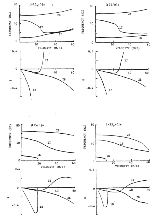
4.4 Flutter analysis diagrams for the four wings with a 15 degree ply fiber angle... ... 82
B.1 - B.7 Static deflection theoretical analysis and experimental
data... ... ... 98
C.1 - C.13 Steady airload theoretical analysis and experimental data...106
D.1 - D.8 Flutter boundary curves...124
D.9 - D.34 V-g method flutter analysis diagrams...132
LIST OF TABLES Table Page 2.1 Assumed modes used in the Rayleigh-Ritz analysis...19
3.1 Different laminate layups used for the test wings ... 60
4.1 Wing divergence speeds...77
4.2 Wing natural frequencies...78
D.1 Flutter data, unswept wing...120
LIST OF SYMBOLS
Symbol
A stress-strain modulus matrix; aerodynamic matrix B stress-bending modulus matrix
b semi-chord of the wing C compliance matrix c chord of the wing Cd coefficient of drag Cf coefficient of force C coefficient of lift
Cm coefficient of moment about the quarter chord
Cp coefficient of pressure
cp center of pressure
D moment-bending modulus matrix EL logitudinal Young's modulus ET transverse Young's modulus GLT shear modulus
g structural damping h vertical deflection K stiffness matrix
kiT non-dimentional torsional stiffness
L lift
P length of wing from root to tip
LA lift associated with bending displacement
LB lift associated with torsional displacement LC lift associated with chordwise displacement M moment per unit length; mass matrix
m mass per unit area
MA moment associated with bending displacement MB moment associated with torsional displacement MC moment associated with chordwise displacement
N force per unit length; chordwise force
NA chordwise body force associated with bending displacement NB chordwise body force associated with torsional displacement
NC chordwise body force associated with chordwise displacement
P distributed force per unit length p distributed force per unt area
Qi generalized enternal force q dynamic pressure
qi generalized coordinate R matrix used to transform K S matrix used to transform K
T kenetic energy
V potential (strain) energy; velocity V, free stream velocity
W weighting matrix
w deflection in the z direction
x y cartesian coordinates z x spanwise axis y chordwise axis a angle of attack
ai beam bending mode constant 0 warping stiffness parameter
Yxy° shear strain tensor at midplane Yi Rayleigh-Ritz mode
6ij delta function
EXo strain tensor in the x direction at midplane SYo strain tensor in the y direction at midplane
ply fiber angle; twist angle
curvature strain tensors
wing sweep angle Poisson's ratio
chordwise deflection air density
Rayleigh-Ritz mode shape part that is a function of x Rayleigh-Ritz mode shape part that is a function of y 9 Kx Ky KXy A LT (
CHAPTER 1. INTRODUCTION
The use of composite materials in aircraft structures has added another design dimension to the aircraft designer. Useful not only for
their high strength to weight ratio but by giving the designer the
ability to vary the force deflection behavior by varying the layup scheme, they have made certain previously impractical design options attractive. In particular, forward swept wings have gained renewed
interest because their major drawback, low wing divergence speeds, can be significantly improved by using tailored composite material in wing construction. A good discussion of this is contained in reference 1.
This project will draw on the work of four previous experimenters at M.I.T.; Hollowell, Jensen, Selby and Dugundji (references 2,3,4 and 5). Those men worked with some of the same wings that were used in this project. They made calculations and ran experiments to determine the
wing stiffness and bending-torsion stiffness coupling, the steady airload deflection behavior and the flutter and divergence speeds at low and high
angles of attack. Using their work as a foundation, we will extend its range by investigating several new ply angle layup patterns and by
investigating aeroelastic properties at 30 degrees forward sweep. Primary interest is in the investigation of divergence and flutter speeds and the wing shapes during those conditions at both low and high angle of attack. Low angle of attack flutter is investigated both theoretically
and experimentally while high angle of attack flutter investigation is
experimental only. We also extend the work of Hollowell on steady airload deflection analysis by including a realistic non-linear lift curve, drag and approximations to three dimentional aerodynamics.
CHAPTER 2. THEORY
2.1 Rayleigh-Ritz Analysis
In this research both static and dynamic analysis are done using the Rayleigh-Ritz analysis technique. We therefore need to formulate an equation of motion for the dynamic analysis and then by setting the time
derivatives equal to zero, we can use the same equation for the static
analysis. Because of the complicated nature of anisotropic material, exact analysis is difficult and often impossible. Therefore I chose an approximate method of analysis, the assumed mode or so called
Rayleigh-Ritz method. This is the same method used by Hollowell, Jensen and Selby (references 2, 3 and 4) who were mentioned in the introduction and in fact, due to the amount of work already done on these wings with
this method I decided to use the same assumed modes im my analysis.
The analysis is linear and assumes all deflections are
perpendicular to the wing in the z direction as shown in figure 2.1.
G = PLY FIBER ANGLE
V.
Note that the ply fiber angle is measured in the opposite direction as
compared to the standard composite material direction.
The basic equation.for the assumed modes is:
n
w(x,y,t) = Y (x,y) q (t)i
i=1
(2.1)
Where Yi(x,y) are the modes. In our case we have five modes so n=5. To get the equation of motion we start with Lagrange's equation.
d ST aT av
dt K 4 r qr
-3q at
Where Q represents the applied loads.
Now we need expressions for the kinetic and potential energies.
For the kinetic energy of a plate we have:
T = ff m (w2 dA
Where m = mass/unit area.
Using equation (2.1) for w we get:
i j S=
f f m
I
iAi
jyj
dA TJ (2.3) (2.4) (2.2)Moving summations and grouping terms:
i j
T
=
Mqq (2.5)where M. =f f Y.my.dA (2.6)
The variational potential energy for a plate is:
6v = ff ( N Se + N 6 + N Y + M 6K + M 6K
x x y o xy xy x x y y
oo
+ M
6K
) dx dy (2.7)xy xy
where using conventional displacement notation: 2 * au a2w xo ax x ax 2 2 av aw = K Yo ay y 2 au 9v - 2(2.8) XY ay + x xy axay
To apply this to anisotropic plates we start with the modulus equations for the general laminate.
{]
i
(2.9)
N = Force/length vector M = Moment/length vector
= strain vector
K = curvature strain vector
A,B,D are the appropiate modulus matrices
Since this is for a plate we assume no strain or shear in the z
direction. For a symmetric laminate, moments about x any y do not cause
strain, only bending so B = 0. In our analysis all loads are in the z direction so N = 0, leaving us with, in expanded form:
Mx
Y
yxy
D11 D12 D 16 D2 1 D2 2 D2 6 D6 1 D 6 6 Kx K y xy (2.10)equation (2.10) for M, integrating with respect to the and using equations (2.8) for the curvatures we get:
variational V = 1/2
ff
[-w,xx -w,yy -2w,xy D1 1 D12 D16 D2 1 D2 2 D2 6 D6 1 D6 2 D6 6 S-W, XX yy (2.11) -2w,xy Using termswhere:
2
w
w, = , etc.
xx 2
expanding this equation and using D21Dx
expanding this equation and using D2 1=D1 2, D16=D61 and D2 6=D 62
V
=1 f f{ D11w, + 2 D1 2w, 1 x xxyy , + D2 222yyw, y 2 + 4D w,
66 xy
+ 4D w, w, + 4D w, w,
j
dA16 xx xy 26 yy xy (2.12)
We now substitute in equation (2.1) for w bring sumations and q's out of the integral to get:
i j
V =I1 qq
ff
D Y Y ,2 i j I 11 xx j xx + 2D 12 Yxx 1'xx Y.j'yy
+ D y., Y., + 4D Y., y, + 4D , y., 22
1
xx yy 661
xy j xy 16 i xx 3 xy+ 4D Y., Y., } dA 26 1 yy ] xy
Finally it is rewritten in the compact form:
i j
1
=- Kij qq
(2.13)
where
K = ff D Yi, Y., + D Yi' y., +4D y, , 11 xx ] xx 22 yy yy 66 i xy j xy
+ D1 2 i'xx' j' +
xxj'yy
+ 2D y, Y.( Y., + y,. Y.,
)
16 1 xx j xy j xxI xy+ 2D26 ( Yi'yyj xy Yyyixy
Note that Kij is symmetric.
Now we can put our expressions for T and V in equation (2.2). for kinetic energy:
Tq
r2
M.. Mij 13 i.q qr iq a4 q'- ja .
+ rq r i ) r usingqi
= ;q ir ;T 1 i -r = - IM q.aqr
2rj
i
r and expanding + - Mir qi 2 ir isince M is symmetric we can sum the two parts:
3T
- = IMr q.
aq rj ]
similarly for potential energy:
S Krjq. (2.15) First (2.17) (2.18) (2.19)
finally d3T 3T dt q= Mrj qj r We note that: aT
and put these into Lagranges equation, using0
and put these into Lagranges equation, using r=i:
M q. + K.,. q. = Q.
1] J 13 J 1
(
j = 1,2,...N) (2.21)in matrix form: M q+ Kq =Q
rre me r (2.22)
This equation will be used to derive all the displacements and motion of
the wings. The five mode shapes used are listed on table (2.1) where
the variables have been separated in the form:
- a
{
sinh Ex 2. cosh (-)
EX Ex - ) - sin(
- ) Ex cos (-- a
sinh 2 Sx ex(
2
sin
(
2-
2
3. sin (-) 3ix 4. sin ( --5x A A4y
1
2 3 c El = 1.8785104 C2 = 4.694091 al = 0.734096 a2 = 1.018466Table 2.1 Assumed modes used in the Rayleigh-Ritz analysis.
The first two are cantilever beam bending modes the second two are
beam torsion modes and the fifth is a chordwise bending mode. You may
notice that modes 3 & 4 do not meet the boundary conditions for a
cantilevered plate at the root where w, x is zero. But the error is small away from the root and an aspect ratio correction for this is made
Mode i (x)
i. cosh ( - - cos ( -- )
in the stiffness matrix terms. Jensen in reference 3 goes through in detail the algebra for working out the mass and stiffness matrix terms and he also derives the torsion stiffness correction factor. In this report only the results are stated.
Mass Coefficients M =mctI M = mc£I 22 2 mct M I 33 12 3 mc£ M 12 44 12 4 4mc£ M 55 I 45 I5 M.. 13 =0 i j Stiffness Coefficients D c 11 K =-I 11
£
3 I6 K =0 12 2D 16 13 2 2 7 D c 11 K = I 22 3 10 2D 26 K =-I 23 2 11 2D 16 24 2.2 12 K 3 4 = 0 4D 16D 16 26 K - I + I 35 2 16 2 17 32 c 4D k 66 2T 2 44 c£ 19 37/2 2D 8D 16 16 K =- I K =- I 14 2 8 25 ci 13 4D 16 45 32 20 32. 8D 12 15 ct I9 4D c 11 K = 55 3 452. 4D 66 33 c2 15 k 1T 2 iw/2 64D 22 64D66 + I + I 22 3 5 3ck 23 c 16D2 6 2 21Where the original values for K33 and K44 were changed using the aspect ratio correction worked out by Crawley and Dugundji (contained in reference 4). where: 2 D11c 8 = 2 48D 66
And the values of knT ( n = 1,2 ) are plotted vs.
8
in figure 2.2.The integrals and their values are listed in table 2.1.
For our particular wings, values of Dij were calculated using the material constants listed below.
EL = 98 x 109 N/m2 ET = 7.9 x 10⁹ N/m2 VLT = 0.28 GLT = 5.6 x 10⁹ N/m2 wing thickness = .804 mm density of wing = 1520 kg/m3
The engineering constants are for Hercules ASI/3501-6 graphite/epoxy for out-of-plane loading (see reference 5 for an explanation on the differences in the engineering constants for in plane and out of plane
2.05 2.00 1.95 1.90 1.85 1.80 1.75 1.70 1.65 1.60 1.55 7.5 7.0 65 S6.0 5.5 5.0 4.5 5 10 15 20 25 30 35 40 45 50 E-3 BETA Figure 2.2 Graph of knT vs.8. 0 5 10 15 20 25 30 35 40 45 50 E-3 E-3 BETA 0 E-3
2.2 Static Deflection Analysis
For static loading, all inertia terms in equation (2.22) are zero so we have left:
(2.23)
Kq = Q
Q is the modal force where:
Qr
=ff
py
rdA
Qr
r dAwhere p is a distributed load per unit area.
For our tests the load was applied at x = £ so we have:
c/2 £ Qr = f
I
p(x,y) 6(x-£) Yr(x,y) dA -c/2 0 c/2 = f P(£,y) Y r(£,y) dy -c/2 (2.24) (2.25)where P is the load per unit length.
load constant in the y direction so we can take P out of the integral. c/2 Q = P
f
Y (a,y) dy r r -c/2 (2.26)Now we need only insert the five modes to get the five values of Qr. They are listed below.
Q1 = 2Pc
Q2 = -2Pc
Q3 = Q4 = Q5 = 0
For the torsional load the test apparatus was assumed to apply load linear to y such that:
p = ay
where a is a constant.
Our equation becomes:
c/2
Q = af y y (,y) dy
r r-c/2
-c/2
Again, putting in the five modes we get: Q1 = Q2 = Q5 = 0 2 ac
Q
3 12 2 ac 4 12The values for Q were calculated and put into equation (2.23) which was
solved for the column vector q. The values of q were then put into
equation (2.1) to get the analytical deflection. The results are shown together with the experimental data on figure B.1 to B7.
2.3 Steady Airload Analysis.
When put in an airstream at a given angle of attack a wing generates airforces, indeed this is its purpose. These airforces not
only support the weight of the airplane but they also bend and twist the
wing itself. This deformation of the wing, in return, by changing the angle of attack, changes the airforces on the wing. The result, shown in
figure (2.3) is a simple feedback system.
dynamic force(a) wing
a 0 c fopressure curve ressure stiffnessstiffness
When the loop converges to a certain value we have the final
deflection. In certain linear theory analysis when the airspeed is increased beyond a critical value the loop does not converge and airforces and deflection increase without limit. This is called divergence. In the real world there are limits to the actual increase in deflection and airforces. They come about due to distruction of the
wing, non-linear stiffness of the wing or non-linear increase of airload with increases in the angle of attack. With our wings the most important
non-linearity, especially at airspeeds at and below the divergence
airspeed, is the non-linear increase of airload with angle of attack. For the steady airload analysis we put in this non-linearity by using the lift and drag curves for a flat plate from reference 10 shown in figure 2.4. reference 10 data 0.8 C 0.6 CD , CL 0.4 CD 0.2 0 4 8 12 16 20 angle of attack
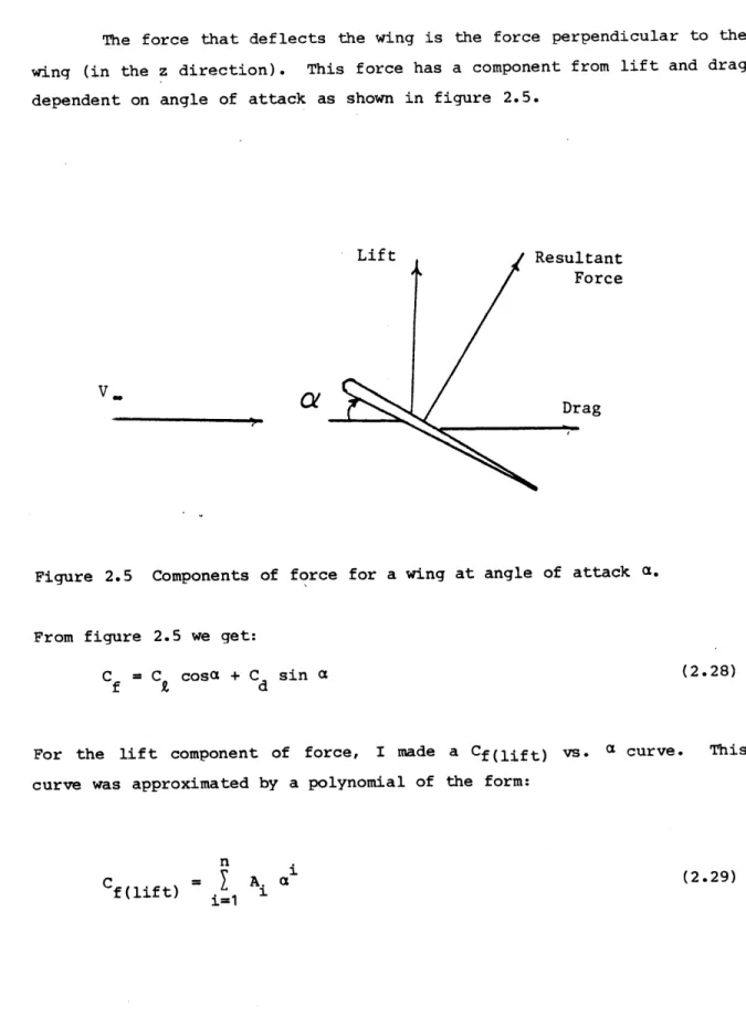
The force that deflects the wing is the force perpendicular to the wing (in the z direction). This force has a component from lift and drag dependent on angle of attack as shown in figure 2.5.
Lift
Vs
Resultant Force
Drag
Figure 2.5 Components of force for a wing at angle of attack a.
From figure 2.5 we get:
(2.28) Cf = CY cosa + Cd sin a
For the lift component of force, I made a Cf(lift) vs. a curve. This curve was approximated by a polynomial of the form:
n
Cf(lift) [ A a i=1
For our purposes n = 4 gave a sufficiently accurate curve. Both the coefficient of force curve and the polynomial approximation are shown in figure 2.6.
4 3 2
C = -37.7072a + 42.472a - 23.167a + 6.6746a
{a
in radians}f(2.30) (2.30) 0.6r Cf(lift) 0.2 reference 10 data - approximation U I 0 4 8 12 16 20 angle of attack
Figure 2.6 Approximation for the
This gives the section coefficient of force from lift as a function of angle of attack but we also need to know the dependance on x and y, or in other words, force distribution on the wing. In reference 4 Selby showed the lift distribution of a rigid wing. This.was used as a guide for modeling the force distribution on our wing. Again a polynomial approximation was used. The distribution in the chordwise y
direction and the approximation are shown in figure 2.7 as coefficients of pressure versus chord.
Approximation equation for force distribution in the chordwise y direction: C = C p p avg 0 3( 0.5 - y 2 (2.31) reference 4 data approximation 0 0.2 0.4 0.6 0.8 1.0 (y + 0.5)/cord
Figure 2.7 Approximation for the Cp curve.
Both the approximation and the theory give 25% chord as the center of pressure in the y direction. Reference 10 shows the coefficient of moment about the quarter chord vs. angle of attack. From this we can calculate the center of pressure movement with changing angle of attack by using:
(2.32)
C
=(py
-y
C
m
cp
.25c
itTo approximate this, a modification was made to equation (2.31). The center of pressure movement and its approximation are shown in figure
2.8.
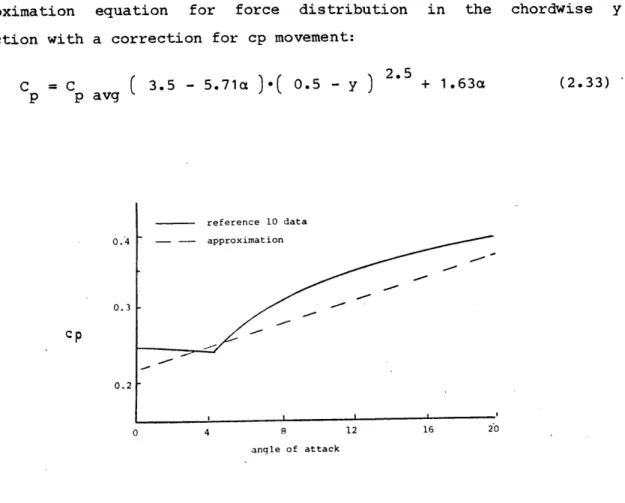
Approximation equation for force distribution in the chordwise y direction with a correction for cp movement:
C = C ( 3.5 - 5.71a )*( 0.5 - y 2.5 p p avg + 1.63a (2.33) reference 10 data 0.4 - - approximation 8 12 16 20 angle of attack
Figure 2.8 Center of pressure movement with changes in angle of attack.
In the spanwise x direction, the lift distribution was calculated using lifting line theory. I used the matrix equation given in reference 7.
1+F
rsinro
sinro
l
c
I
S 81 sin
i
Nwhere: a = 2w 0 c = chord £ = semi-span x = cos ( m m -r = ( 2n - 1
)
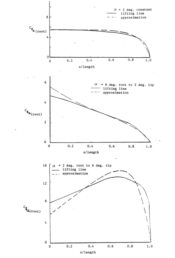
n = column number m = row numberThe lift distribution was calculated for three cases, a rigid wing
at 2 degrees angle of attack, a wing with positive twist of 4 degrees
with the root angle of attack at 2 degrees and a wing with negative twist of 4 degrees with the root angle of attack at 6 degrees. These three cases span a good part of the low angle of attack deformation conditions for our wings. The three cases along with the approximation used are plotted in figure 2.9. The same approximation was used in all cases.
Note that C£a(root) = C/a(root)
Approximation equation for force distribution in the spanwise x direction:
x 9(2.35)
C = C 1.111 1 -( ) } (2.35)
8 C (root) 4 0 C (root) C t(root) ( = 2 deg. constant lifting line - - - approximation 0 0.2 0.4 0.6 0.8 1.0 x/length
S = 6 deg. root to 2 deg. tip lifting line approximation 0.2 0.4 0.6 0.8 1.0 x/length 0 0.2 0.4 0.6 0.8 1.0 x/length
Figure 2.9 Spanwise lift distribution for various twist conditions for a
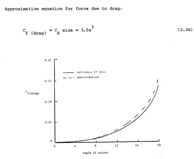
Finally, for drag I used the curve from reference 10 shown in figure 2.10 with its approximation. Drag was assumed to be a function of angle of attack only and not of x and y .
Approximation equation for force due to drag:
Cf. (drag) 0.20 0.15 Cf (drag) 0.10 0.05 0 Cd d sina = 3.5a3 (2.36) reference 10 data approximation 4 8 12 angle of attack 16 20
Figure 2.10 Change in force due to drag with changes in angle of attack
Putting all the approximations together we get a two dimentional force
distribution on the wing where:
p=Cp .Axy
4 3 2 C = A + A3a + A2a + A1 a *
1.11[
1
-
(
] {
(3.5-
5.71a
[ 0.5 - (
25
+
1.63a
}
3 + 3.5a (2.37)For a, the vast majority of the twist () is from the first assumed torsion mode so I used equation (2.38) for a = aO + 0 *
q3
a(x) = a + sin- ( - ) sin( '
)
(2.38)This completes the distributed force coefficient term. Multiply this by dynamic pressure and we get the distributed force per unit area. This was put in the Rayleigh-Ritz analysis to get the modal force Q.
X c/2
Qr =f
f
f(x,y) y(x,y) dx dy (2.40)0 -c/2
The equation was solved on a digital computer by numerical integration. Then equation (2.23) was solved for q. Solutions were calculated for three airspeeds 5, 11.5 and 16 meters per second at angles of attack from
2 to 20 degrees at 2 degree increments. If 16 m/s was higher than the
wing divergence speed, I omitted the calculation at that speed. For 5
m/s three iterations were sufficient, for 11.5 m/s five iterations were sufficient and for 16 m/s up to seven iterations were used. The results for a straight wing (A = 0) are plotted along with experimental data in figures C.1 through C.13.
2.4 Wing Divergence Analysis.
Basically a wing diverges when the aerodynamic forces from increased angle of attack due to twist are stronger than the resisting
forces from the wing's torsional stiffness. When wings are swept,
bending also causes changes in angle of attack while bending stiffness resists these changes.
To calculate divergence, therefore we need to relate the stiffness forces to the aerodynamic forces. In matrix form the torsional stiffness equation is :
{ 0
= [ c
z E(
[ C
I
M (2.41)If the forces and moments can be combined to make a force at a specific
chordwise point we get:
S)
= [C ( F ) (2.42)The aerodynamic forces for a station along the span are:
a
= cC ,q q = dynamic pressure)
(2.43)In matrix form we have:
L } =q cC
}
(2.44)Where
[
W]
is a weighting matrix for the stations chosen and contains the appropiate amount of spanwise length to make the running lift .thelift for the area covered by the station. In this case lift is the force in equation (2.42) so we have:
So
}
=[
c
]
q
[
]
cC
}
By use of an aerodynamic scheme we will get:
a =A(cC )
Where A is the aerodynamic operator. In matrix form:
Sa
=[
A
]
cC
or:
(2.48)
C,}=[A]
a
putting this into equation (2.45) we get:
-1
)
=q[c[
[
[A]
{a
We note that a a + 0
Where a0 is the rigid or root angle of attack. To calculate divergence, we set a0 = 0, so we get:
(2.49) (2.45)
(2.46)
(2.47)
and
-1
1 -1
-{ q
o }=[
C[
[ ]{}A
(2.51)This we recognize as a characteristic value equation where for the first
characteristic value, say X, we have:
= -- (2.52)
(divergence)
This is the form of the solution to the divergence problem. We need
only determine the three matricies [ C ], [ W ] and [ A ]. Because the compliance matrix will be made to match the aerodynamic matrix we will determine the aerodynamic matrix first.
To derive the aerodynamic matrix I used the Weissinger L-Method.
This method and its theoretical foundation are outlined in reference 7.
The final matrix form for lift symmetric about the fuselage is:
a{
=
[
A]
{
cCS}
(2.53)DeYoung and Harper is reference 11 write this equation in the form:
(m-1)/2
a = a G (2.54)
v vn n
n=1
The avn terms are the terms of the aerodynamic matrix and Gn is a form of the chord times the lift coefficient. They have graphed values
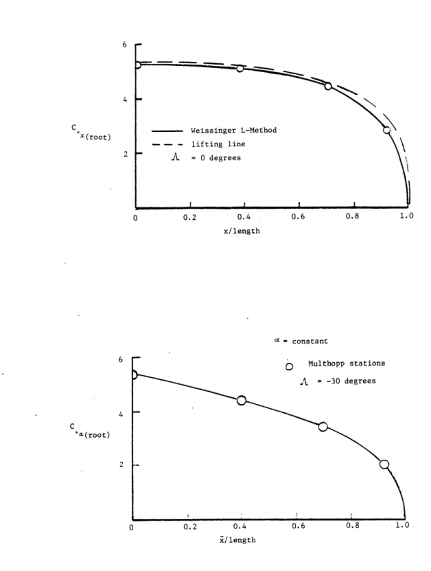
for the aerodynamic matrix terms versus wing geometry giving a 4 x 4 aerodynamic matrix. Although the swept wing was of primary interest in the divergence analysis, I constructed an aerodynamic matrix for both the straight wing and a 30 degree swept forward wing ( A = 0, -30 ). With the aerodynamic matrix and known angle of attack, a simple simultaneous solution of the four equations gives the section coefficient of lift. The results are shown for constant angle of attack for both straight and sweep forward wings in figure 2.11. The lifting line results for the straight wing are coplotted for comparison.
The four stations used by Harper and DeYoung are the four so called Multhopp stations and are at:
x
= .9239, .7071, .3827, 0.0
for the stations 1, 2, 3 and 4 respectively. This method puts the bound vortex at the quarter chord while meeting boundary conditions at the three quarter chord. This is equivalent to saying the force is at the quarter chord while the angle of attack is measured at the three quarter chord position. This gives us the necessary information to match the compliance matrix to the aerodynamic matrix.
Also reference 7 gives the terms in [E] when using the Multhopp stations.
To calculate the compliance matrix we will use the coordinate system in figure 2.12.
x (root) 0.2 0.4 0.6 0.8 x/length = constant m(root) i/length
Figure 2.11 Lift distribution in the spanwise x direction using the Weissinqer L-method
V,
A
---y y
Figure 2.12 Swept forward wing coordinate system.
In our case all loads can be considered point loads applied at quarter chord in the y-axis and at the Multhopp stations in the x-axis. This reduces equation (2.24) to:
4
(2.55)
j=1 F.x.,y.
1
(x ,
1(x2 2 ). Y1( x4' 4)2 x2'
2 "") 2(
x4
4)
75(Yx2
2 ..
5 x4'y 4
Let's call the matrix that premultiplies {F}, [R], so
{
Q} =[R] Fin short form:
(2.57)
Now putting that aside for the moment, let's get a relation for twist
angle 0. Using small twist angle assumptions we can say:
e
= - - (2.58)(2.59) = - cosA - a sinA
For w we substitute in equation (2.1)
5 ai (x,y)
yi
(x,y)0=- a( - cosA + sinA ) qi
i-=1
(2.60)
To get the twist at the four Multhopp stations we use the x-axis position of the station for 3j and three quarter chord for j where j is the index for the Multhopp station. This gives us:
1 \ Q2 5 F F2 F 4
5 ay x.,y yi
(x.,y
e
= - + +cosA - sinA)q.j
i=i=1
in expanded form a1(Xl,I )ay1
x
1
)
1xy 4)ay
2( x
1
ay
2(x
2f
2)
ay x2 a2(x4 4 .... ay5(x2 ,y 2)ay
a5 (x4,y 4 ) ay a5s(x11Y)a
ax Dy5(x4 4) 93Fa.
a7
1 (x2'Y 2 ) ay1(x 4'y 4)a 3E
a 2(x IYl .... ax ay2(x 2,' 2) ....ay
2(x4'Y 4) .... 37' ql 92 sinA q5Calling the matrix that premultiplies {q} in equation
have in short form:
S) =[
s]
{q}
(2.62), [S], we (2.63) (2.61) 01 2 e4 cosANow using equation (2.23) where we premultiply by the inverse of [K].
SK
q}= [K
Q }
(2.64)putting this in equation (2.63) we have:
{ }= [s]] K
{Q
(2.65)putting equation (2.57) into equation (2.65)
{ }=[s][K] [R ]{F (2.66)
We can now see that our compliance matrix is of the form:
[c] =[s][K] [R]
Finally, we put equation (2.67) in equation (2.51) giving us:
-1 -1
1
){
[s][K] [R][W][A] {}q
(2.67)
(2.68)
This equation was solved in a digital computer and the first characteristic value gives the divergence velocity. With some of the wings with negative bending torsion coupling, for the straight wing case, the divergence velocity was imaginary. This indicates that according to
linear theory .the wing will not diverge. The results of the analysis are shown together with experimental data in table 4.1.
2.5 Flutter Analysis.
For flutter analysis, I used the well known V - g method. In this method, structural damping (g) is introduced into the equation of
motion. since solutions of the equation of motion represent the neutral
stability condition solution, when g is negative the wing is stable.
When g is positive we see that damping is required for neutral stability. Flutter occurs when g is equal to the actual damping of the
structure.
Assuming harmonic motion q(t) = q eiLt
),
the equation ofmotion is:
2 ist
SK - M ) itQ (2.69)
First we need to derive the unsteady aerodynamic forces in terms of Q in equation (2.22). We will do this by deriving the variational work (W) and put that in terms of Q by using equation (2.70).
5
6W = I Q q (2.70)
n-1 r r
The general form for 6W is:
1 c/2
6w = f f p 6w dydx (2.71)
0 -c/2
The term p6w can be separated into three components and their respective displacements; lift, moment and camber force about the
midchord (L6h, M60 and N6). where: c/2 L = f p dy -c/2 c/2 M = - f yp dy -c/2 c/2 N = I 5 p dy (2.72) -c/2
V
+1
4-91?'
Figure 2.13
convention.
Swept wing coordinate system and the displacement sign
Using figure 2.12 (reproduced here) for the swept wing geometry and
figure 2.13 for the displacement sign convention, then relating the
assumed modes to the different displacements we can write:
h = (x) q1 + 2(x) q2 (2.73)
1 dh
=- 3(x)3 + 4( ) q4 cosA + d sinA
}
(2.74)55 (x) q5 (2.75)
Using equation (2.73) we can write equation (2.74) as:
8
e
-
{
[
0
3(x)
q
3 + 4(x)
q4cosA
1
+ - q + - q2 sinA
}
(2.76)Putting equation (2.72) in equation (2.71) we get:
W =
f
L Sh dx +f
M 6e dx +f
N 6~ dx (2.77)0 0 0
Now putting equation (2.73), (2,75), and (2.76) into equation (2.77) and rearranging terms we get:
d1(x) 6W = { fL 1 (X) dx - sinA fM d dx 6qi 1 f d 1 0 sd# 2(x) + f L 2 (x) dx - sinAI M d dx } 6 q2 0 cosA f M 43(x) dx 6q 3 0 C f M 4(x) dx
Sq4
0 (2.78) +f
N t5(x) dx 6q 5 0Now, taking the relations worked out by Spielberg for 2-D incompressible
aerodynamic theory in reference 12, and adapting them to our swept wing
case, we get equations for lift, moment and camber force.
Ab B Cb
M = wp2 be ( M h + MB + M C ) cosA
2 3 it h
N =
wrp
be(N
+ N + N ) cosAAb B Cb (2.79)
non-dimentional complex functions of reduced frequency k = Wb/V, given by: L =1 A i L B k 2C (k) -i k SC(k) 2C(k) + i X + k 2 k 1 L = C 12 C(k) 2C(k) -i 3k 2 k C(k) k 1 i M =---B 8 2k C(k) C(k) +i 2k + 2 k i C(k) 1 M -1 + C 2k 6k 2 k C(k) k 1 C(k) N =----NA 1 2 3k i C(k) C(k) N =-+i + B 3k 6k 2 3k 1 j C(k) 1 C(k) N =--i + C 36 1 8k 2 2 2k 3k
where C(k) is the Theodorsen function.
49
(2.80)
and the functions
These equations assume harmonic motion such that:
iwt
h(x,y,t) = h(x,y) e , etc. (2.81)
Putting equations (2.79), (2.73), (2.76) and (2.75) in equation (2.78),
using equation (2.70) and rearranging terms we get for Qi:
Q = pw2b3 iwt
LA 2 dx (x)
I [ cosA - f
(
(X))
dx - cosa sinA LB 1(x) d dxd (x) - cosA sinA M d A d x L + [ cosA f 1 ((X)
#2(x)
0 2 dO (x) 2 l (x) dx + b cosA sin A M(
)i
q1 0 d#2(x) dx - cosA sinA LB f 1 (x) d dx 0 da1(x) - cosA sinA M d 1 ( 2(x) dx 0 2 + b cosA sin A M B Sd (x) 0 d2 (x) d dx ] q2 dx 2 *cos 2 A (x) (x) b cos A sinA d (x)
c LB f 1 x) 3 (x) dx - c B dx 3 (x) dx ] q3
2 2 d1 (x)
cos ALB I ) 4(x) dx -bcos A sinA 1 f(x) d
c L 1 4 c B dx 4
L d (x)
+ [ cosA -
f
(x) (x) dx - cosA sinA Mc I d) dx]
qb 5 C dx 05 5 2 3 iwt Q2 = wpw b e LA
{
cosA
- f
2(x)
- cosA sinA MA/
0 d (x) W1(X) dx - cosA sinA LBI
2(x) dx dx d2(x)d 02 Wd dx 1(x) dx d 2(x) d 1(x) + b cosA sin2A M d(x) d x ] q B dx d d rx 1 L 2 d2 (x)+
[
cosA - 2 (x) dx - cosA sinA LB / 2 x dx dxb 2 LB J 2 dx
2 2 d(x)
A LLB B (x) x) (x) dx b cos A sinA MB f 2)
3(x) dx .q
cos A L 2(b cos A sinAM f 2
0 0 d 2 (x) + [ cosA do 2 W + LC f 2(x) 5(X) dx - cosA sinA MC f di 5 (x) dx ] q5 2 3 iwt Q3 - wPW b e 2 2 c A s (x) dx- b cos A sinA
S[
E A 3 x) 1 x)x c1 MB £ f 4)3(X) dl (x) d dx ] q1 + cos A M 3(x) c A 0 b cos A sinA2
(x)
2dx-
cM
BB d (x) X 2 ) f 3)x) d2 dx ] q2 0 _ [ b cosA A-
2 M f 03(x)
dx ] q3
0 £ - b MB f 3 (x) 4(x) dx ] q4 c 0cos A + c M f 3 (x) (x) dx
]
q 5 0 Q4= p2 3 iwt Q4=--Wpbe
* 2 cos A A MA f4 (x2
+ cos A + MA f t4(X) 0 2 a (x) 1BJ 4 dx]
0 2, d ( b cos A sinA _ 2(x) 2 (x) dx c MB f 4 (x) d dx ] q2 0 3 b cos A -2 B f *4() 03(x) dx ] q3 c 3 2 b cos A --2 MB f ( ) dx ] q4 c + cos2A S MC f 4 () 5(x)dx q5 0 2 3 iwt 5 = WpW b e d xS
cosA NA5 x)
1()dx
- cosA
sin
N5
x dr
i
Sd2~(x) +
[
sA Af
5(x) 42(x) dx - cosA sinA NB f 5) d dx]
q2 0 0 2 -[oL
NB 5(x) 3(x) dx] q3 0 (2.82) 2 [ cos A B 5 x) 0 *4(x) dx ] q4 + Nc f 5(x) dx] q 5 0Inorder to integrate with respect to the variable substitution;
x = E cosA
x we use the
(2.83)
This makes the limits of integration: 0 to X/cosA or 0 to
1,
which is the original distance in the unswept case. Now we write Q in the form:5
q
=wp2b3e
i t IAij q j=1
where the terms of [A] are:
2
cos A 2 2
A11 - b LA I - cos A sinA L I - cos A sinA M I
11 b A 1 B 24 A 24
2 2 1
+ b cos A sin A M I
Bt 25
A = 2 2
A = - cos AsinA L I - cos AsinA M I +
12 B 26 A 27 2 2 b cos A sin A
a
MB 28 3 cos A 13 c B 2 3 cosA 14 c LB 31 2 cos A 15 b C 33 3 b cos A sinA + M -9 c B 3 b cos A sinA 2 - cos A sinA M C 34134 2 2A2 1 = - cos A sinA L I -cos sinAM I +
21B 27 A 26 2 2 b cos A sin A X MB 28 2 cos A 2 2
A22 b LA I - cos A sinA L I - cos sinA M I
22 b A 2 B 35 A 35 2 2 + b cos A sin2 A 3 cos A = --
5
L LB B I3737 cos A A = -A L I 24 c B 39 1 M - I B 36 3 b cos A sinA MB 3 b cos A sinA + M c B 30 32 A 2 3 138 140I N VUTS V SOO -I N q V SOD LSv
0
- = sv0 V soo V s o q 0 I W + VUTs V Soo q 6£ V 0 V £S o o LE w 0 VI W V IOW V soo 8EI HN~
o S VuTs V soo q £ 0£I gW Vu T s o + V soo q IVI 3 vu VSo£ ZI DN VUTS V ,soo 0 = VT 0 EI '6W = V~ V soo q LEI'6
vW
Z V V Soo£ 6Z 0f LE V soo LI D Dq q _ Sq v r s O = V V =2 cos A 2 A5 2 52 = b b N A I 41 - cos A sinA N B 42I24 cos A 5 3 c B 43 cos 3A A N 14I 54 c B 44 2 cos A A5 5 55 bos NC b C I 1 5 (2.85)
The integrals and their values are listed in table A.1.
From this point on, the flutter analysis for the swept wing is the same as the analysis for the straight wing as give by Hollowell and Dugundji in reference 5.
Equation (2.84) is put in equation (2.69) and both sides are devided by eiwt.
2 2 3
K q - w M q = wpw b A q (2.86)
In the normal fashion for the V - g flutter analysis, structural damping (g) is introduced by multipling K by (1 + ig). We define a complex eigenvalue Z as:
1 + ig (2.87)
we define a new matrix B as:
3
B = M + rpb A (2.88)
Finally putting equations (2.87) and (2.88) in equation (2.86) we have, a standard form, complex eigenvalue problem:
{
-Z K I q = 0 (2.89)This equation was solved on a digital computer. Selected values of reduced frequency k were used to calculate the aerodynamic matrix.
The eigenvalues Z were used to get the oscillating frequency w, the structural damping required g, and the velocity V, according to equations
(2.90). 1 W Re(Z) Im(Z) g - (Z) Re(Z) (2.90)
The flutter velocity was chosen as the velocity at which the structural damping required to maintain neutral stability became zero on any of the five modes. The associated value of w is the flutter frequency. To simplify calculation of the Theodorsen function C(k), I used the R. T. Jones approximation given in equation (2.91).
2
C 0.5 p + 0.2808 p + 0.01365 p + 0.3455 p + 0.01365
Note that by using large values of k the output frequency will be
the natural vibration frequency of the wing in an atmosphere of density p. This technique was used to get the theoretical natural frequencies.
This analysis was done for all thirteen wings. The results are
CHAPTER 3. EXPERIMENTS 3.1 Test Wing Selection
The criteria defining desireable characteristics of the test wings are the same criteria used by Hollowell in reference 2. they are:
a) The wings should have a wide range of bending-torsion stiffness coupling.
b) The wings should have constant chord, thickness, sweep and zero camber.
c)The wings should flutter or diverge within the 0-30 m/s speed
range of the available wind tunnel.
d) The wings should be small enough to be made with the available
equipment for manufacturing graphite/epoxy plates at M.I.T..
e) The wings should not sustain any damage under repeated large static and dynamic deflections.
To give a good cross section of the range of bending-torsion coupling and stiffness, both balanced and unbalanced
laminates were made at three different ply angles. In table 3.1 we can see the range covered.
[+15 2/0]s [+302/0]s [+452/01s increased [±15/0]s [±30/0]s [±45/0]s negative [T15/0]s [T30/0]s [T45/0]s [-152/0] [-302/0 s (-452/01s increased positive bending-torsion coupling
Table 3.1 Different laminate layups used for the test wings.
bending-torsion coupling
The [02/90]s serves as the only uncoupled example. Positive
bending-torsion coupling means when the wing is bent in the positive z direction the wing will twist in the positive twist direction. The positive twist direction is the same direction as positive angle of
attack. Because of the layup convention shown in figure 2.1, +0 fibers
on the outside plies result in negative bending-torsion stiffness
coupling and vice versa.
3.2 Static Deflection Tests
The goal for the static deflection tests was to test the
wings under static loads of pure force and pure moment. Also the loads should be large enough to cause large deformations, inorder to identify
any non-linearities in the stress-strain relations and thus identify the
limitations of our linear analysis.
The static deflection setup is shown in fig 3.1. It is
Figure 3.1 Static deflection test apparatus.
--i.--
- .
~---*--X--~X-l --..
~--
3~-C- -C_-
- -~----
I-
---constructed of sturdy wood beams with metal rulers attached to the
insides of the top horizontal beams. These rulers were used to measure horizontal deflection while a carpenters square was used to measure vertical deflection. To minimize measuring error we extended pins from a
balsa wood clamp at the wing tip. threads ran from two eyelets on the balsa wood clamp around pulleys clamped to the side of the test apparatus
Figure 3.2 Static test stand with a moment being applied.
and down to weight holders. One eyelet was at the wing leading edge
while the other was at the trailing edge. To apply a force the pulleys and weights were put on the same side of the test apparatus while to apply a moment the pulleys and weights for the leading edge were put on
one side and those for the trailing edge were put on the other side. (see
figure 3.2)
We applied force in increments of approximately 0.2 N up to 1.0 N then in double increments till a bending deflection of approximately 12
cm. Moment was applied in a similar manner with initial increments of .0075 NM till approximately 0.2 NM. This caused a twist of from 8 to 22
degrees depending upon the torsional stiffness of the wing.
3.3 Wind Tunnel Test Setup.
We did the wind tunnel tests in the M.I.T. acoustic wind tunnel.
This tunnel has continuous flow with a 1.5 by 2.3 meter free-jet test
Figure 3.2 M.I.T. wind tunnel test setup.
section 2.3 meter long, located inside a large anechoic chamber. The
tunnel speed range is continuously variable up to approximately 30 m/s. Velocity was sensed by a pitot tube in the throat immediately before the
test section and registered on a electrical baratron.
a turntable machined from alluminum and mounted on a rigid pedestal. The mount for the wing is attached to the top of the turntable. The
turntable allows rotation of the wing to angles of attack from -4 to 20 degrees while the top of the wing mount allows wing sweep in increments
of 15 degrees from -45 to +45 degrees of sweep. The photo shows the wing in -30 degrees of sweep. In our testing only the -30 and 0 degrees of sweep positions were used. Slightly below the base of the wing we
Figure 3.4 Looking down on a test wing by using a mirror.
mounted a flat disk to provide smooth airflow past the model, a good background for the vertical photos, a place to mount the angle of attack control rod and also a place to mount a terminal for the strain gauge wires. The disk was also labeled for each test to identify the still and
figure 3.4. We hung a mirror over the wing to get the pictures looking down on the wing. Figure 3.5 shows the location of the video camera, still camera, strobe and floodlight. When it was necessary to "slow down" the motion during a flutter test we used a strobe, otherwise
floodlights were used. By checking the strobe frequency we could determine the wing flutter frequency.
The scale on the disk was used to measure wing tip bending and twisting. It is graduated in 1 cm increments. Since viewing angle and position affect the picture you see when looking at the test wing through the mirror, tests and calculations were made to adjust the apparent displacement to the actual displacement. These adjustments were then
applied to the data readings off the pictures.
Fig.3.5 Equipment used to illuminate and record test wing movement.
-3.4 Natural Frequency Tests.
Hollowell, Jensen, and Selby (references 2,3 and 4), already
tested many of these wings for their natural frequencies. Also they have shown that the theoretical analysis using the five Rayleigh-Ritz modes gives accurate results for the first and second bending and first torsional natural frequencies. Therefore instead of doing extensive
natural frequency tests we did a simple initial deflection vibration test. With the wing mounted for the wind tunnel test we gave it an
initial deflection in twist and bending, released the wing and recorded the oscillations on the strip chart recorder. The resulting oscillations contained strong first bending with weak second bending and first torsion oscillations.
3.5 Steady Airload Test.
The steady airload tests were to be run at zero sweep and wind speeds of 5, 10 and 15 m/s. However after investigating the results and
repeating selected tests we determined that the baratron on the original tests was indicating a lower airspeed than the actual tunnel airspeed. Using a different and accurately calibrated baratron during the repeat
tests we determined that the actual tunnel airspeeds on the original
tests were 5, 11.5 and 16 m/s within a tolerance of 0.5 m/s.
To run the test, first we set the tunnel speed, then using the
strain gauge readings we zeroed the angle of attack by setting it so that the average bending and torsion gauge readings were zero. (The tunnel, especially at higher speeds has enough turbulence to cause small irregular deflections in the wing causing temporary non zero readings even at zero degrees angle of attack.) The wing was then run through angles of attack from 0 to 20 degrees at two degree increments. We made records of each incremental stop by strip chart records of the strain gauge readings, still photos and video recordings. Following the
completion of tests at one airspeed we repeated the procedure at the next
was not increased at that speed. Some of the wings will flutter at 16
m/s at any angle of attack so that portion of the test for those wings
was omitted.
3.6 Flutter Boundary Tests.
A flutter boundary is a curve plotted on a airspeed vs. angle of
attack graph for a particular wing where one side of the graph,
invariably the lower airspeed side, is a flutter free area while the other is a flutter area. Previous experimenters had found the flutter boundaries of many of the wings in our tests. Our goal was to complete these tests for all the wings at both no sweep and 30 degrees forward
sweep. Our procedure was to set the airspeed, zero the angle of attack
and then run through the different angles of attack checking for
flutter. When we encountered any flutter, either bending or torsion, we
made strip chart recordings and checked the frequency with the strobe.
After finishing tests at that airspeed the angle of attack was reduced, the airspeed was increased by 1 m/s and the test procedure was repeated. When airspeed is increased to the point where the wing flutters at all angles of attack or the maximum tunnel speed is reached final readings are taken and the test for that wing is complete.
3.7 Flutter Test.
Our goal was to observe the actual shapes of the wing during both
low and high angle of attack flutter. In particular we wanted to concentrate on observing the wing tip, getting not only qualitative data but actual measurements of the bending and twisting seen at the tip. We chose 1 degrees AOA for the low angle of attack flutter and 10 degrees
AOA for the high angle of attack flutter. Using data from the previously
run flutter boundary tests, we set the airspeed at the flutter speed and then set the angle of attack. If the flutter was intermittent or of very small amplitude we increased the airspeed by as much as one meter per
all the flutter cases with the various wings, the wings fell into two
main categories; ones that had flutter dominated by torsion oscillations
and ones that had flutter dominated by bending oscillations. The torsion flutter frequencies were in the area of 30 to 60 hz. This is much to
fast to see clearly with the eye and even using a video camera the motion will come out blurred on each frame. However since the motion is steady
in a periodic sense it can be captured by use of a strobe. The strobe flash frequency is set near the flutter frequency by visual observation, resulting in flutter motion that can be viewed at apparent slow motion. The images also record relatively well on a video camera. The strobe has a very fast flash during which the wing moves very little, giving a sharp but brief image. the video camera elements, however, have a certain
amount of persistency, holding the image after the flash has stopped. So
when the video camera scans it has an image nearly all the time even though the flash lasts less than 1/1000th of a second. For this reason
the video pictures made using the strobe provided all the quantitative
data on the high frequency flutter. When the flutter-frequency was low, as in bending flutter, we took video pictures using alternately strobe
and floodlight. Under floodlighting the video picture was clear but still to fast to take measurements. While recording under the strobe the video recording was blank with an occational brief picture. However,
when individual frames were viewed in still motion, the floodlight video
pictures were easy to interpret. The strobe lighted video pictures were another matter. When the strobe had flashed a single video frame was
clear, otherwise it was blank. With the strobe flashing at about 5 hz
and the video camera scanning at 30 hz there is one clear frame followed by approximately 6 blank frames. This large spacing between good video frames along with the slow flash rate in relation to random turbulence induced motion in the tunnel made it difficult to know when we had a picture of the wing at maximum deflection. Therefore the floodlight video pictures provided the bulk of the data for the bending flutter
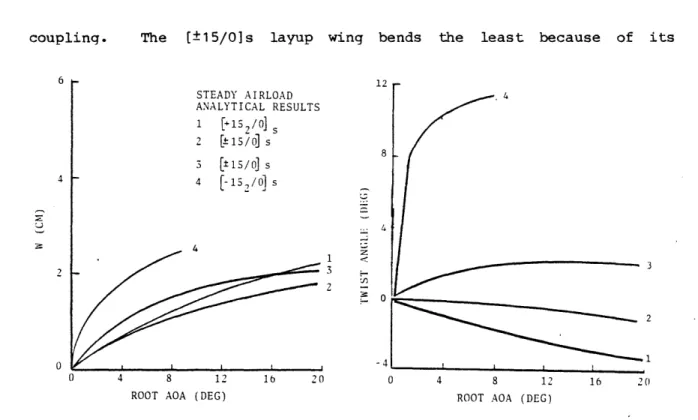
![Figure B.2 [+152/0]s layup wing, static deflection.](https://thumb-eu.123doks.com/thumbv2/123doknet/13895387.447740/99.1188.261.982.152.751/figure-b-s-layup-wing-static-deflection.webp)
![Figure B.5 [±30/0]s layup wing, static deflection.](https://thumb-eu.123doks.com/thumbv2/123doknet/13895387.447740/102.1188.209.1006.142.739/figure-b-s-layup-wing-static-deflection.webp)
![Figure B.7 [±45/0]s layup wing, static deflection.](https://thumb-eu.123doks.com/thumbv2/123doknet/13895387.447740/104.1188.264.1031.94.747/figure-b-s-layup-wing-static-deflection.webp)
