Lidar observations of ozone changes induced by subpolar air mass motion over Table Mountain, California (34.4°N)

HAL Id: insu-03041869

https://hal-insu.archives-ouvertes.fr/insu-03041869

Submitted on 2 Feb 2021

HAL is a multi-disciplinary open access

archive for the deposit and dissemination of

sci-entific research documents, whether they are

pub-lished or not. The documents may come from

teaching and research institutions in France or

abroad, or from public or private research centers.

L’archive ouverte pluridisciplinaire HAL, est

destinée au dépôt et à la diffusion de documents

scientifiques de niveau recherche, publiés ou non,

émanant des établissements d’enseignement et de

recherche français ou étrangers, des laboratoires

publics ou privés.

Lidar observations of ozone changes induced by subpolar

air mass motion over Table Mountain, California

(34.4°N)

Thomas Mcgee, Paul Newman, Richard Ferrare, David Whiteman, James

Butler, John Burris, Sophie Godin, I. Stuart Mcdermid

To cite this version:

Thomas Mcgee, Paul Newman, Richard Ferrare, David Whiteman, James Butler, et al.. Lidar

ob-servations of ozone changes induced by subpolar air mass motion over Table Mountain, California

(34.4°N). Journal of Geophysical Research: Atmospheres, American Geophysical Union, 1990, 95

(D12), pp.20527-20530. �10.1029/JD095iD12p20527�. �insu-03041869�

JOURNAL OF GEOPHYSICAL RESEARCH, VOL. 95, NO. D12, PAGES 20,527-20,530, NOVEMBER 20, 1990

Lidar Observations of Ozone Changes Induced by Subpolar Air Mass Motion

Over Table Mountain, California (34.4øN)

THOMAS J. MCGEE, • PAUL NEWMAN, l RICHARD FERRARE, 1 DAVID WHITEMAN, 2 JAMES BUTLER, 3 JOHN BURRIS, 1 SOPHIE GODIN, 4 AND I. STUART MCDERMID 4

Between October 15 and November 8, 1988, the Goddard Space Flight Center mobile stratospheric lidar was in place at the (JPL) Table Mountain Facility (located at 34.4øN, 117.7øW) for the purpose of intercomparing with the JPL lidar permanently stationed at the observatory. During the course of the intercomparison both lidar systems detected a significant change in the vertical profile of ozone lasting for several days. An analysis of meteorological data available from the National Meteorological Center has shown this change to be dynamical in origin due to the transport of subpolar air over Table

Mountain.

INTRODUCTION

In October 1988 an ozone measurement intercomparison was held at the Jet Propulsion Laboratory (JPL) Table Mountain Facility in the San Gabriel Mountains east of Los

Angeles (34.4øN, 117.7øW). The purpose behind the inter-

comparison was to test the performance of two stratospheric lidars: the permanent JPL system housed at Table Mountain, and the mobile lidar built at NASA's Goddard Space Flight Center (GSFC). Both systems were funded by the NASA Upper Atmosphere Research Program for eventual inclusion

in a network for the early detection of stratospheric change.

Such a network is to be set up for the ground-based detection of long-term stratospheric trends [Watson, 1986] and would include a number of stations located at appropriate latitudes around the globe. During the course of the intercomparisons period, both lidars independently detected a large and sud- den change in the ozone concentration between 24 and 35 km. The maximum ozone depletion occurred at 27 km on October 20. This event was followed by a slow return to what was considered to be a "normal" profile. This paper reports the observations and the interpretation of the atmo- spheric phenomenon taking place from October 18-24.

EXPERIMENT

Both lidar systems have been previously described in detail [McDermid et al., 1990a, McGee et al., 1990]. Briefly, both are differential absorption lidars using XeC1 excimer lasers to generate the on-line wavelength at 307.9 nm. The systems differ, however, in the manner in which the off-line wavelength is generated. The GSFC instrument transmits

the third harmonic of a Nd-YAG laser at 354.7 nm. This laser

operates at 16.5 Hz., corresponding to every fourth shot of the excimer. The JPL lidar uses stimulated Raman scattering (SRS) in molecular hydrogen to generate 353 nm radiation.

•NASA Goddard

Space

Flight Center, Laboratory

for Atmo-

spheres, Greenbelt, Maryland.

2NASA Goddard

Space

Flight Center,

Laboratory

for Oceans,

Greenbelt, Maryland.

3ST Systems

Corporation,

Lanham,

Maryland.

4jet Propulsion

Laboratory,

Table Mountain

Facility,

California

Institute of Technology, Wrightwood.

Copyright 1990 by the American Geophysical Union.

Paper number 90JD01878. 0148-0227/90/90JD-01878505.00

Both of the off-line wavelengths have ozone absorption cross sections which are about 3 orders of magnitude lower than the on-line wavelengths. Because of the large solar flux at the transmitted wavelengths, the lidar systems currently make ozone measurements only at night. The lidars were physically separated by approximately 300 m during the intercomparison, but this separation was insufficient to avoid interference between the systems. Consequently it was necessary to operate the lidars sequentially rather than simultaneously. A detailed analysis of the data from the two lidars has been made and published elsewhere [McDermid et al., 1990b]. The two systems agree very well between 20 and 40 km. Because of this excellent agreement and the fact that the systems were operated over slightly different time inter- vals, the lidar data for each evening were combined to yield a single profile. These averaged profiles are discussed in this

paper.

RESULTS AND DISCUSSION

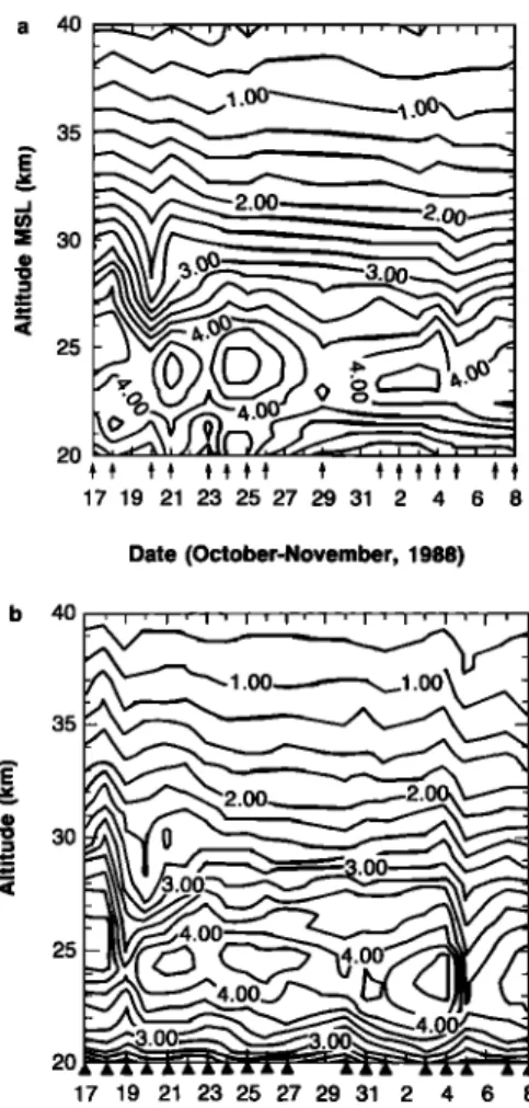
The contour plots of Figure 1 contain the GSFC (Figure la) and the JPL (Figure lb) data recorded during the intercomparison. The days on which data were taken are noted at the base of each figure. Data between these dates were obtained by interpolation. Between 20 and 40 km, the agreement between the lidar data is quite good, as can be seen from the similarity between the plots. The plots show a marked depletion in ozone number density between 24 and 32 km, occurring between October 18 and October 24. The largest change was measured at 27.5 km by both lidars on the night of October 20. There was approximately a 30% change in ozone number density observed at this altitude between October 18 and 20. The depletion at 27.5 km is also accom- panied by a downward shift in the ozone maximum of about 2 km. There is some recovery in the measured profiles after October 20, but the measured ozone concentration at these

altitudes did not return to the levels of October 18.

Also evident in the figures is a sharp feature detected in

the measurements made November 5. This feature was

noted by the rocket, balloon, and satellite measurements made on the same day. An analysis of the available National Meteorological Center (NMC) data along with the chronol- ogy of the ozone soundings indicated that the dynamics of the ozone decrease occurred too rapidly to be captured by the available meteorological data, and so is not addressed in this publication.

20,528 MCGEE ET AL.' LIDAR 0 3 OBSERVATIONS a 4O 35 •: 30 25 20 17 19 21 23 25 27 29 31 2 4 6 8 Date (October-November, 1988) 40 , , , , , , , , , , 30 17 19 21 23 25 27 29 31 2 4 6 Date (October-November, 1988)

Fig. 1. Contour map of the (a) GSFC and (b) JPL ozone data

between October 17 and November 8, 1988. Dates on which data

were obtained are noted along the base of the figure. Other data were obtained by interpolation. Units are 1018 m -3.

Since the photochemical lifetime of odd oxygen is greater than 12 days at altitudes below 35 km [Garcia and Solomon, 1985], it is unlikely that the rapid depletion observed be- tween October 18 and 20 is photochemical in origin. In order to assess the transport effects involved in the change, it is necessary to analyze the available meteorological data. Radiosonde measurements were obtained from Point Mugu, California (34.2øN, 119.1øW) and from San Nicholas Island, California (33.3øN, 119.5øW), while global stratospheric analyses were obtained from the Climate Analysis Center within the National Meteorological Center. These NMC analyses have been previously described in detail [Gelman et al. , 1986].

Transport changes in ozone occur by either vertical or

horizontal advection, or some combination of the two. For vertical advection, potential temperature 0 can be used as a conserved vertical coordinate. Potential temperature is de- fined as the temperature 0 a parcel of air would acquire if it were adiabatically brought to 1000 mbar

0 = T(Po/P) • (1)

Here, T is the temperature at the starting pressure P; P0 =

1000 mbar, and y - 2/7 (the ratio of the gas constant of dry air to the specific heat of dry air at constant pressure). The

diabatic heating rate Q can be expressed in terms of potential

temperature:

dO/dt- Q (2)

Under the condition that the diabatic heating rate is small (this is generally true; average diabatic heating rates for October at 35øN latitude in the altitude range 24-30 km have been calculated to be less than 1 K/day [Rosenfield et al.,

1986]), potential temperature remains constant and air par- cels then move quasi-adiabatically. Therefore an air parcel

will tend to remain on a surface of constant potential temperature (which is an isentropic surface). For this rea-

son, potential temperature is superior to geometric altitude as a vertical coordinate, since a parcel will remain on a potential temperature surface, whereas it can move over a large range of geometric altitude.

The horizontal motion of air masses can be best followed

using Ertel's potential vorticity (EPV) on isentropic surfaces

[Andrews et al., 1989]. Potential vorticity is calculated from the following expression:

00

EPV = -g(• + f) (3)

OP

where g is the gravitational constant, • is the relative vorticity, f is the planetary vorticity, and 0 is the potential temperature. EPV is in units of km/(kg s) and has a typical

mid-latitude

value

of approximately

10 x 10

-5 for the middle

stratosphere. EPV is conserved for periods of the order of 1-3 weeks in the stratosphere when diabatic processes and frictional forces are small. Potential vorticity for a given isentropic surface has well-defined horizontal gradations. Typically, there are large values of EPV in the polar region, and smaller values in the tropics. The boundary between polar values and mid-latitude values is generally very sharp [Clough et al., 1987; Juckes and Mcintyre, 1987]. The equator-pole gradient is not uniform, but it is small in both the polar and equatorial regions and is sharply peaked in the

mid-latitudes. This sharp EPV gradient defines the boundary

between polar and mid-latitude air.

Because rapid ozone changes took place between October 18 and 20, the profiles obtained on these two nights have been used in the dynamical analysis. Radiosonde data from Point Mugu have been combined with the lidar number density data to form the volume mixing ratio. This is employed because unlike number density the mixing ratio is not influenced by local vertical motions when it is viewed on a potential temperature surface (i.e., mixing ratio is thus conserved along an isentropic surface). Figure 2 plots the calculated mixing ratio as a function of altitude. If vertical motion is the only mechanism considered, the mixing ratio shown in Figure 2 suggests that the ozone profile has been vertically lifted by 3-4 km in the 24- to 30-km altitude range. Since the potential temperature is approximately conserved on this time scale, a local lifting of 3-4 km would induce an adiabatic cooling of approximately 30 K. The plot of tem- perature versus altitude shown in Figure 3 shows that there has been a change of only 4-6 K at altitudes of interest over the days in question. Since the predicted adiabatic cooling calculated from the lifting of the ozone profile is inconsistent with the observed temperatures, vertical advection is not a significant source of the ozone reduction. The slight cooling

MCGEE ET AL.' LIDAR 0 3 OBSERVATIONS 20,529 40 i [ [ [ 35 E 30 _.- 25 2O 15

'"•m

18

Oct.

1988

Ozone Mixing Ratio (ppmv)

Fig. 2. A plot of the ozone volume mixing ratio as a function of altitude for October 18 and 20. The mixing ratios were constructed from the combined lidar ozone profiles and the temperatures ob- tained from balloon sondes launched from Point Mugu and San

Nicholas Island.

observed in the radiosonde data indicates a small lifting of

about 0.5 km.

The Ertel's potential vorticity plots derived from the NMC data show horizontal motion as the primary source of the ozone depletion. Figure 4 shows volume ozone mixing ratio

as a function of potential temperature and indicates that the

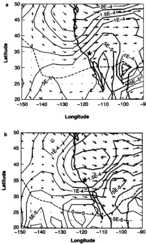
largest change in ozone mixing ratio occurred at 700 K. Figures 5a and 5b show the EPV fields on the 700 K

isentropic surface for October 18 and 20, respectively. The

thin solid lines are the EPV contours, while the thick solid

line delineates the transition from easterly to westerly winds. The wind vectors are also displayed to indicate the direction of EPV movement. The winds are northwesterly in the North Pacific and eventually become westerly over the western coast of the United States. Figure 5a shows a large high of potential vorticity extending southwestward from

Vancouver Island into the Pacific Ocean. The winds advect

this high potential vorticity systems southeastward, and by

October 20 (Figure 5b) the disturbance has moved into a

position over the central portion of the western United States. In the process of this movement, potential vorticity

values have doubled over Table Mountain. Note that the

lOOO

900

-

_ /•"' __

18

Oct.

1988

Ozone Mixing Ratio (ppmv)

Fig. 4. Ozone volume mixing ratio as a function of potential

temperature.

volume mixing ratio generally remains constant on an isen-

tropic surface along the contours of constant potential vor- ticity. Therefore since the large values of potential vorticity

observed over Table Mountain on October 20 are normally at latitudes substantially north of 34 ø , the observed ozone

values are characteristic of early winter subpolar ozone, not

mid-latitude ozone.

The horizontal ozone gradient can be estimated from the decrease in ozone mixing ratio between October 18 and 20.

a 50 45 4O :3 35 3O 25 20 -150

- \,, "

---

20

0ct.

1988

Fig. 3. The balloon temperature profiles measured on October 18

and 20. b 50 45 4O 35 30 20 -150 -140 -130 -120 -110 -100 -90 Longitude

Fig. 5. Ertel's potential calculated for the 700 K potential tem- perature surface for (a) October 18 and (b) October 20. Table Mountain (34øN, 117øW) is denoted by a star. The heavy dashed line is the boundary between easterly and westerly winds.

20,530 MCGEE ET AL.: LIDAR 0 3 OBSERVATIONS

The decrease in ozone mixing ratio was 3-4 ppmv at the 700 K potential temperature surface. The mixing ratio on Octo- ber 18 is approximately associated with potential vorticity values near 7.5 x 10 -5 while on October 20 it is associated

with potential

vorticity values near 1.5 x 10

-4. If the

average distance between these EPV contours is taken to be 400 km, then the mixing ratio gradient near Table Mountain

is approximately-1.0

x 10 -2 ppmv/km.

Using

the 10-mbar

solar backscatter ultraviolet (SBUV) mixing ratios of Naga- tani et al., [1988] we can estimate an average gradient of

-1.6 x 10 -3 in the zonal mean at 35øN.

This mean

gradient

is 6 times smaller than that estimated from the lidar and

potential vorticity measurements.

The disparity between the lidar/EPV-estimated gradient

and the SBUV mean data is almost certainly due to the SBUV monthly and zonal averaging. As is shown in Figure 5, the vortex is far from zonally symmetric. Hence the zonal averaging produces a smeared image of the rather sharp vortex boundary. The large depletion between October 18 and 20 indicates large zonal asymmetry in the mid-latitudes, and the large horizontal ozone gradients.

SUMMARY

We have made iidar measurements of the vertical profile of ozone above Table Mountain and observed a large de- crease in ozone density between 24 and 32 km. The pertur- bation lasted several days and was observed independently by both the JPL and GSFC lidars. An analysis of the available meteorological data has shown that the decrease was caused by an influx of subpolar air over the lidar site. A much sharper gradient between high-latitude air and mid- latitude air was measured by the lidars than had previously been reported based on satellite measurements.

Acknowledgments. The funding for both lidar instruments was provided by the NASA Upper Atmosphere Research Program. We would particularly like to thank the staff from the JPL Table Mountain Facility for their assistance throughout the intercompari- son. P.N. and R.F. are University Space Research Associates.

Clough, S. A., N. S. Grahame, and A. O'Neil, Potential vorticity in the stratosphere derived using satellites, Q. J. R. Meteorol. Soc.,

111,335, 358, 1985.

Garcia, R. R., and S. Solomon, The effect of breaking gravity waves on the dynamics and chemical structure of the mesophere and lower thermosphere, J. Geophys. Res., 90, 3850-3868, 1985. Gelman, M. E., A. J. Miller, K. W. Johnson, and R. M. Nagatani,

Detection of long-term trends in global stratospheric temperature from NMC analyses derived from NOAA satellite data, Adv. Space Res., 6, 17-25, 1986.

Juckes, M. N., and M. E. Mcintyre, A high resolution, one-layer model of breaking gravity waves in the stratosphere, Nature, 328,

590, 1987.

McDermid, I. S., S. M. Godin, and L. O. Linqvist, Ground-based laser dial system for long-term measurements of stratospheric ozone, Appl. Opt., 29, 3603-3612, 1990a.

McDermid, I. S., S. M. Godin, L. O. Linqvist, T. D. Walsh, J.

Burris, J. Butler, R. Ferrare, D. Whiteman, and T. J. McGee,

Measurement intercomparison of the JPL and GSFC strato- spheric ozone lidar systems, Appl. Opt., in press, 1990b.

McGee, T. J., D. Whiteman, R. Ferrare, J. Butler, and J. Burris,

STROZ Lite: NASA/GSFC stratospheric ozone lidar trailer ex- periment, Opt. Eng., in press, 1990.

Nagatani, R. M., A. J. Miller, K. W. Johnson, and M. E. Gelman, An eight-year climatology of meteorological and SBUV ozone data, NOAA Tech. Rep. NWS 40, 1988.

Rosenfield, J. E., M. R. Schoeberl, and M. A. Geller, A computa- tion of stratospheric diabatic residual circulation using an accu-

rate radiative transfer mode, J. Atmos. Sci., 44, 859-876, 1987.

Watson, R. T. (Ed.), Network for the Detection of Stratospheric Change, Report of the Workshop, Upper Atmosphere Research Program, NASA, Washington, D.C., 1986.

J. Burris, R. Ferrare, T. J. McGee, and P. Newman, Laboratory for Atmospheres, NASA Goddard Space Flight Center, Greenbelt,

MD 20771.

J. Butler, ST Systems Corporation, 4400 Forbes Boulevard,

Lanham, MD 20707.

S. Godin and I. S. McDermid, Table Mountain Facility, Jet Propulsion Laboratory, California Institute of Technology, Wright-

wood, CA 92397.

D. Whiteman, Laboratory for Oceans, NASA Goddard Space Flight Center, Greenbelt, MD 20771.

REFERENCES

Andrews, D. G., J. R. Holton, and C. B. Leovy, Middle Atmo- spheric Dynamics, pp. 115, 139-141, Academic, San Diego,

Calif., 1989.

(Received October 31, 1989;

revised August 16, 1990; accepted August 20, 1990.)