Directionally controlled open channel microfluidics

HAL Id: insu-02474428

https://hal-insu.archives-ouvertes.fr/insu-02474428

HAL is a multi-disciplinary open access

archive for the deposit and dissemination of sci-entific research documents, whether they are pub-lished or not. The documents may come from teaching and research institutions in France or abroad, or from public or private research centers.

L’archive ouverte pluridisciplinaire HAL, est destinée au dépôt et à la diffusion de documents scientifiques de niveau recherche, publiés ou non, émanant des établissements d’enseignement et de recherche français ou étrangers, des laboratoires publics ou privés.

Directionally controlled open channel microfluidics

Golak Kunti, Jayabrata Dhar, Anandaroop Bhattacharya, Suman

Chakraborty

To cite this version:

Golak Kunti, Jayabrata Dhar, Anandaroop Bhattacharya, Suman Chakraborty. Directionally con-trolled open channel microfluidics. Physics of Fluids, American Institute of Physics, 2019, 31 (9), pp.092003. �10.1063/1.5118728�. �insu-02474428�

Directionally Controlled Open Channel Microfluidics

Golak Kunti,1 Jayabrata Dhar,2 Anandaroop Bhattacharya,1 and Suman Chakraborty1*

1

Department of Mechanical Engineering, Indian Institute of Technology Kharagpur, Kharagpur, West Bengal - 721302, India

2

Universite de Rennes 1, CNRS, Geosciences Rennes UMR6118, Rennes, France

*

2

ABSTRACT

Free-surface microscale flows have been attracting increasing attention from the research community in recent times, as attributable to their diverse fields of applications ranging from fluid mixing, particle manipulation, to bio-chemical processing on a chip. Traditionally, electrically-driven processes governing free surface microfluidics are mostly effective in manipulating fluids having characteristically low values of the electrical conductivity (lower than 0.085 S/m). Biological and biochemical processes, on the other hand, typically aim to manipulate fluids having higher electrical conductivities (0.1S/m). To circumvent the inherent limitation of traditional electrokinetic processes in manipulating highly conductive fluids in free surface flows, here we experimentally develop a novel on-chip methodology for the same by exploiting the interaction between an alternating electric current and an induced thermal field. We show that the consequent local gradients in physical properties as well as interfacial tension can be tuned to direct the flow towards a specific location on the interface. The present experimental design opens up a new realm of on-chip process control without necessitating the creation of a geometric confinement. We envisage that this will also open up research avenues on open-channel microfluidics; an area that has vastly remained unexplored.

3

I. INTRODUCTION

Free-surface problems often pertain to situations in which the interface topology is not known a-priori and is determined from the coupled solution of the non-linear field equations.

1–4

In many engineering and geophysical applications, such as flow in open channels, bubbly flows, hydrodynamics, rivers, lakes, boiling, cavitations, sea waves etc., free-surface flow is encountered. The physics of such flows becomes truly fascinating when other external fields, such as electrical fields, are employed to manipulate the free surface. 5–7

Recent studies on free-surface flows in miniaturized devices have promised potential applications in fluid mixing, chip cooling and cleaning.8,9 Such progresses have been possible as a consequence of a phenomenal recent advancements in microfluidic and nanofluidic device fabrication processes,10,11 which brought to focus several reduced-scale electrokinetic transport mechanisms12–17 and their derived technology.18 Recently, electric field-driven actuation has emerged tremendously in microscale transport system due to its several advantages, such as chip scale integrability, no moving part, high reliability, portability, etc.19–24 Alternating current electrokinetics (ACEK) stands as an effective choice for manipulating fluid flows in several devices of these kinds, considering its excellent on-chip integrity, low excitation voltage and precise controllability over miniaturized scales. 25–27 Efficient and effective fluid mixing, 28–31 pumping, 32–36 particle manipulation, 37–41 and two-phase flow42,43 have been demonstrated with success, by employing ACEK mechanisms of flow manipulation.

Alternating current electroosmosis (ACEO) flow may arise through the interaction between the induced charges in the electrical double layer (EDL) and tangential component of the electric field.44,27 The pertinent operating parameters that control the efficacy of an ACEK process primarily include the frequency of the electrical pulsation and electrical conductivity of the working fluid. Beyond a threshold frequency (>100 kHz45–47) and electrical conductivity (0.085S/m48), ACEO remains inefficient for fluid manipulation. However, a wider operating regime of the device may be potentially explored, by exploiting thermal gradients in the system, through the realization of an intricate interplay between the temperature-depended electrical properties and the electrical stresses.49–52 Such mechanisms have been successfully used for transporting fluids in confined geometrical pathways.33,53,35 The performance of such pumping mechanisms has been successfully demonstrated widely varying geometrical and physical conditions such as grooved channel,33,45 thin film heater,54,55 DC (direct current) biasing56 and two-phase electrical signalling.36

Demands of deploying geometric confinements, such as microchannels, may often impose fabrication and implementation restrictions for applying electrothermal flows in conjunction with simple on-chip configurations for practical applications ranging from chemical and thermal processing to biomedical technology. Evading these limitations, here we report the first experimental results of generating controlled

4

directional free-surface flows on a microfluidic chip by deploying an intricate interaction between the electrical and the thermal field, without necessitating the fabrication of a confined geometric passage. Interestingly, the thermal field exploited for this purpose is not externally imposed but is intrinsically induced through electrical Joule heating. This, in turn, imposes gradients in conductivity and permittivity, inducing free charges into bulk fluid. These mobile charges effectively set the free-surface fluid into motion. On the other hand, gradients in fluid density and free-surface tension generate buoyancy force and thermocapillary force, respectively which interplay with electric forces, and tune the free surface flow in a rather intriguing manner. With suitable arrangement of the electrodes on the chip, one may impose patterned variations in the temperature gradient over the domain, leading to the inception of free-surface flow in a preferential direction. In what follows, we thoroughly discuss the experimental setup, the methodology, and the theoretical basis of the present study in Section II. Then, we focus on our key findings and associated discussion in the Section III. Finally, we summarise with the principal conclusions of this study in Section IV.

II. MATERIALS AND METHODS A. Experimental method

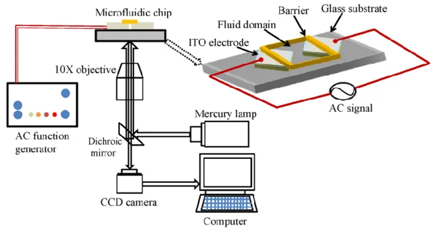
The concept geometry is shown in Fig. 1, where, for simplicity, we have taken two pieces of indium-tin-oxide (ITO) electrodes. These electrodes are embedded on a clean glass to form a microfluidic chip. The thickness of the ITO coating is 150 nm. While deployment of more numbers of electrodes with tunable spacing may offer better control over the free surface flow, we do not attempt to elucidate those additional results here, with a sole purpose of demonstrating the essential physical concept.

In a demonstrative example we first refer to, the minimum gap between the electrodes is _{65μm and is increasing from the centre to the edges of the electrodes.} The height of water and glass are 1.1 mm, and 1 mm, respectively. The electric field is maximum at the narrow gap and it gradually decreases towards the edges of the electrodes. As mentioned previously, Joule heat is generated due to the presence of an external electric field; hence, it will be stronger in the region of high electric field. A maximum temperature will thus be generated over the electrode gap where the electrode spacing is minimum. As the electric field strength decreases with increasing electrode spacing, temperature also decreases towards the wider spacing. The established temperature gradient therefore shows its peak at the narrow gap (maximum temperature occurs around the electrode tip) and decreases towards the wider gap. Far away from the electrode gap, temperature rise does not occur due to weak electric field strength. This temperature gradient drives the fluid towards the narrow gap of the electrodes where temperature is high. Glasses with ITO electrodes (thickness: 1.1 mm)

5

were kept on a clean glass substrate. To maintain the gap between the electrodes and to make a barrier, we used a sealing element around the electrodes (see Fig. 1). The barrier is far away from the narrow gap so that end effects do not disturb the flow field. KCl (Merck Life Science Pvt. Ltd.) electrolyte solution of electrical conductivity 0.099-1.92 S/m was used as fluid medium. AC field was employed using a function generator (33250A, Agilent). Fluorescence microscopy imaging technique was adopted to track the fluorescent particle (diameter 1 μm, FluoSpheres@carboxylate, Life Technologies Pvt. Ltd) motion. An inverted microscope (IX71, Olympus) and a CCD (charge-coupled device) camera (ProgRes MFcool) were used to observe and record the fluid motion, respectively.

FIG. 1. Schematic of experimental set up of free-surface flow. Fluid domain is filled by KCl solution.

On activation of electric filed a hot spot is generated at the centre of the fluid domain and fluid flows towards the hot spot.

B. Theoretical basis

Here, we have considered quasi-electrostatic field,57,58 where induced magnetic field can be neglected. The spatial distribution of the voltage () in the domain can be obtained solving the following equation: 47,59





   (1)

where  is the electrical conductivity. Electrothermal forces arise from the gradients of electrical properties which are generated by the temperature gradient in the electrolyte. Application of electric field causes Joule heating, which can be expressed as a volumetric source term in the energy equation, as:

2 2

, p

E C T k T

6

where E ( E E,  ) is the electric field, V is the fluid velocity,  is the mass density, p

C is the specific heat at constant pressure and k is the thermal conductivity. Generated

gradients in conductivity and permittivity are    (  / T) T and      ( / T) T,

respectively. For aqueous solutions, these gradients, typically are

1

( /T) / c_  0.4% K and 1

( /T) / c_ 2% K . 60 Inhomogeneities in electrical properties generate mobile charges in the electrolytic medium, as governed by the

following expression for the volumetric charge density:

( ( / ) ( / )) / ( ) ;

q     T   T  i  T E   / t i;  _{being the frequency of the} AC signal. 61

Combined effects of induced mobile charges and electric field generate electrothermal forces, where the volumetric force density is given by: 61–63

2

0.5 .

E q 

F E - E (3)

The equation governing fluid motion is then given by:

 

where  is the fluid viscosity. F_E is the time average electrothermal forces 61,64,65.  is the charge relaxation time. The buoyancy force reads Fb  g= (/ T) TgTg, where

 is the thermal expansion coefficient. Thermocapillary forces (FTH) may alter the fluid

velocity due to surface tension gradient with temperature. The expression of the

thermocapillary force can be found in Ref. 66,67, which is





F .  is the thickness of the interface

between water and air. T is the gradient of interfacial tension. In addition, electrical stresses at the interface may also play role in perturbing the velocity field.

For low fluid velocity (~10-4 m/s) the convection heat transfer is negligible compared to conduction heat transfer. Therefore, from the energy balance (Eq. (2)) one may obtain

2 2 ~ E lr T k   (5)

where lris the reference length scale. Due to negligible effect of inertia force, viscous force (~u l/ _r2) is balanced by the electrothermal, buoyancy and thermocapillary forces and can be expressed by

2 2 3 / ~ ( ) T r r r T u l E g T l           _ _{  } (6)

7

The reduced order form of the above equation can be explored to avail a scaling analysis of the system, the results of which are shown in Fig. 3. Here, u_ris the reference velocity. Further, gradients of conductivity and permittivity can be written as

60,61 1 / ( )( ) 0.01 1 / ( )( ) 0.001 T c T T T T c T T T                   _{ }    _            (7)

Eqs. (5), (6) and (7) can be combined to evaluate the reference velocity as a function of electric field as 4 2 ~ r u AE BE (8) where,





  . The typical values of the physical

quantities used here, consistent to experimental values, are given in Table 1. Apart from the scaling between various forces, some important dimensionless groups, such as Reynolds number, Peclet number, capillary number have a range of 0.001, 0.1-0.01, and 0.5-0.1-0.01, respectively, in this problem.

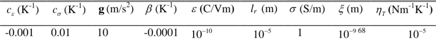
Table 1. Values of the parameters used in the scaling analysis.

c_(K-1) c_ (K-1) g (m/s2)  (K-1) (C/Vm) lr (m)  (S/m) (m) T(Nm

-1

K-1)

-0.001 0.01 10 -0.0001 10

10 105 1 10968 105

Some other parameters which are not mentioned in the table are : k ~ 0.1W/mK,

0.001

 Pa.s, and ~ 1000kg/m3.

8

FIG. 2. (a) and (b) show the tracking of particles to measure fluid velocity (Multimedia view) [URL: ... .1].

(c) depicts vector field of the flow and shows direction of the flow. The operating parameters are electrical conductivity: 0.36 S/m, peak to peak voltage: 10 V, and frequency: 1 MHz.

In this section, we discuss the influence of operating parameters on controlled directional free-surface flow. To illustrate the flow field characteristics, we have shown the experimental results of particle tracking and the corresponding velocity vector field (at a plane that is 30 μm below the electrode surface) in Fig. 2 (Multimedia view); the parameters used in the investigation are mentioned in the figure caption.

We start by considering two particles A and B in Fig. 2a (Multimedia view). As the electric field is switched on, both the particles traverse towards the narrower edge of the electrode. This can be seen from Fig. 2b (Multimedia view), where electric field and thermal field are the strongest. Directions of motion of the particles A and B are

t =10 s t =10.04 s

(a) (b)

9

shown by arrow. The electric field strength is maximum at the narrow gap of the electrodes. Accordingly, the temperature is highest at the narrow gap of the electrodes. Using a thermocouple temperature was measured above the narrow gap. A temperature rise of 7.5 °C was found. The present configuration deals with low Reynolds number flow where inertial effects are less compared to the viscous and electrothermal forces. Hence, in the energy balance, thermal conduction scales with the Joule heating source, so thatT : E2. Therefore, high local temperature gradients prevail at locations having high local electric field strength. The temperature sharply drops as one traverse from the narrow gap to the wider gap. This implicitly induces high temperature gradients within the system at close proximity to the electrode edge. The strong thermal field is effective in generating strong electrothermal forces. Besides, due to the local change in density, a buoyancy force is also induced that controls recirculation near the electrode gap. Further, variation in surface tension due to temperature gradient generates thermocapillary flow. The direction of this flow takes place from a higher temperature location to a lower temperature location. Therefore, thermocapillary force may oppose the electrothermal forces at some locations.

The corresponding vector field, depicted in Fig. 2c, shows overall converging flow characteristics due to the combined effects of electrothermal, buoyancy, and thermocapillary forces consistent with such electrode arrangement. The resultant fluid motion takes place from the cooler region to hotter region which implies that the electrothermal force is dominant over the thermocapillary force. The arrows show the flow direction of the directional free-surface flow. It is clear that fluid motion takes place from wide region to narrower region at this plane, owing electrothermal effects. Strong electrothermal forces bring the surrounding fluid towards the centre of the electrode system. It is noted that at this observation plane, the flow flux is directed towards the central location of the chip. Another flow flux from the centre to the outward direction is inevitable due to the fluid continuity constraint in the domain and such a flux is actually observed at the free surface near the fluid-air interface.Here on, we proceed to further explore the involved dynamics of electrothermally driven free-surface flow in more details in the subsequent discussions.

10

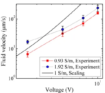
FIG. 3. Log-log plot of fluid velocity with applied voltage for two different conductivities

0.93,1.92

 S/m at frequency 1 MHz. We also show the velocity vs voltage plot (solid line) obtained from scaling analysis with index 2.9.

Our experiments have demonstrated that the flow velocity is strongly dependent on the applied voltage and the solution conductivity. Fig. 3 highlights the variation in fluid velocity with the applied voltage (log-log plot) for conductivity values of 0.93, 1.92 S/m, whereas the frequency of electrical pulsation is kept at 1 MHz. Here, we have taken average flow velocity of the tracer particles. We have also shown the velocity vs voltage plot (solid line) obtained from scaling analysis. It is clear that the flow velocity drastically increases with the voltage. Stronger the electric field, higher will be the temperature gradients due to Joule heating which increase the various forces in the system. From the scaling analysis (Eq.(8)) fluid velocity due to electrothermal forces varies with fourth power of the electric field strength. Accordingly, dependence of the fluid velocity on voltage is u_ACET ~4(since

~ /

E  g). However, in the system, other forces, such as buoyancy force and thermocapillary force influence the overall velocity and interplay with electrothermal forces. From regression analysis of the experimental data of velocity versus voltage for four different conductivity values ( 0.099, 0.36, 0.93and 1.92 S/m), the experimentally obtained index of electric field dependence of flow velocity is 2.69, resulting in some deviations from the scaling analysis (it is 2.9 for scaling). This deviation can be attributed to the fact that other phenomena viz. dielectrophoresis, evaporation alter the flow field with some lesser extent. As a result, experimentally obtained velocity slightly deviates from the scaling argument.

11

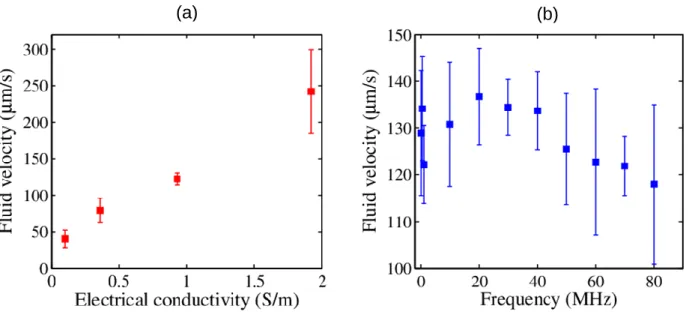
FIG. 4. Experimentally obtained fluid velocity as a function of (a) conductivity for peak to peak voltage

10 V and frequency 1 MHz; (b) frequency for peak voltage of 10 V and conductivity 0.93 S/m. Error bars depict the standard deviation of the velocity data. Due to large fluctuation in the velocity at high conductivity (= 1.92 S/m) the error bar is quite large for  1.92S/m as compared to error bars at other conductivities.

In Fig. 4a, fluid velocity variation with the electrical conductivity of the solution, for applied voltage 10Vpp and frequency 1 MHz, is presented. It is noted that fluid

velocity varies almost linearly with the electrical conductivity of the solution. One can see that in the energy equation, the temperature gradient varies as  T . Since from force balance it was found that fluid velocity is proportional with T, it is expected that fluid velocity has linear dependence with electrical conductivity. Fig. 4b depicts the influence of the frequency on the fluid velocity, for conductivity of 0.93 S/m and voltage of 10V . The pertinent electrokinetic forces comprise Coulomb force and dielectric force. Coulomb force directly depends on operating frequency whereas dielectric force is independent of the frequency. These two forces oppose each other and form an angle between the relevant force vectors in the phasor space. A crossover frequency, at which the magnitudes of the two forces are equal, may be obtained as:

/ 2 (1 2 / )

c

f      . Thus, it depends on the physical property of the fluid medium. For conductivity  0.93S/m, the crossover frequency becomes 718.5 MHz. Below this frequency, the Coulomb force dominates over the dielectric force and owing to complete saturation of free charges the net force almost becomes invariant with the frequency. Our experiments were conducted in the frequency range of 0.1 to 80 MHz. Frequencies beyond 80 MHz were not imposed due to limitation of the function generator. The adopted highest frequency is quite below that of the crossover frequency. Accordingly, the net force in the free surface flow remains almost constant. The measured velocity data shows imperceptible variations in the mean flow velocity, with the lowest and highest velocities in the tune of 118 μm/s and 136 μm/s ,

(b) (a)

12

respectively. Therefore, alteration of fluid velocity with AC frequency agrees well with the theoretical predictions.

In the previous discussions, we have analyzed the characteristics of directional free-surface flow and effects of various important parameters. It is seen that by tuning the directionality of the imposed thermal field, it is possible to direct the free surface flow along a specified location. In the following discussion, we show the application of the concept to direct the fluid through an open channel. To form an open channel flow configuration, we consider a taper electrode arrangement whose entry (at wider gap of electrodes) and exit (at narrow gap of electrodes) appear as inlet and outlet of the open channel, respectively.

Fig. 5 (Multimedia view) shows the particle tracking and velocity vector to estimate the velocity magnitude and direction of the flow, respectively. The tracking particles (particles A, B, and C) move along the tapper path (shown by green arrow). As we have mentioned earlier that the temperature is increased from wider gap to narrower gap, fluid flows from wide region to narrower region along the tapper channel. Corresponding vector field shows the flow direction.

13

FIG. 5. (a) and (b) show the tracking of particles to measure fluid velocity (Multimedia view) [URL: ... .2].

(c) Depicts vector field of the flow and shows direction of the flow. The parameters are electrical conductivity 0.36 S/m, peak to peak voltage 10Vand frequency 1 MHz.

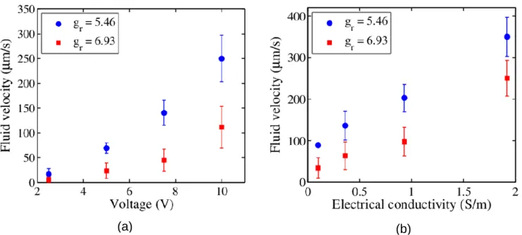
To make an assessment of dependency of fluid velocity with electrode spacing and characteristics of tapering, we have shown mean fluid velocity at inlet of the open channel for two different cases: (i) widths of the narrow gap go 65μm and wider gap

355μm

i

g  (ii) widths of the narrow gap g_o 80 μm and wider gap g_i 555μm (Fig. 6). Subscripts i and o stand for inlet and outlet, respectively. For cases (i) and (ii) the gap ratios are gr a, 5.46and gr b, 6.93, respectively. The results are shown as a function of voltage (Fig. 6a) and fluid conductivity (Fig. 6b). Although increase in electrode gap from narrow to wider region is sharp for case (ii) (since g_{r b,} g_{r a,} ), the mean fluid velocity is higher for case (i). Fluid velocity depends not only on how fast electrode spacing becomes narrow to wide but also on the actual electrode spacing. In the present scenarios, effect of electrode spacing is much significant than the drastic change in electrode spacing. For the case (i), the electrode spacing is smaller compared

t = 20 s t = 20.04 s

(a) (b)

14

to case (ii). The electric field strength is higher for case (i) which causes a much sharper temperature gradient that induces large electric forces. As a result, fluid velocity is high in case (i). An important point to be to be mentioned at this juncture that due to occurrence of electrolytic reaction at high voltage (~ 12.5 V) for g_r 5.46,

1.92

  S/m we have taken upper limit of voltage as 10 V (safe operating voltage i.e., free from electrolytic reaction).

FIG. 6. Fluid velocity as a function of (a) voltage and (b) conductivity for two different electrode

arrangements: case (i) electrode gap at inlet and outlet gi355μmand go65μm, respectively; case

(ii) electrode gap at inlet and outlet gi555μmand 80μm, respectively. For (a) other parameters are:

conductivity 1.92 S/m and frequency 1 MHz. For (b) other parameters are: peak to peak voltage 10 V and frequency 1 MHz. Error bars show the standard deviation. From the value of error bars, it is confirmed that due to large fluctuation in velocity measurement at higher voltage the standard deviations are also high at higher voltages.

From Figs. 6a and 6b it is evident that fluid velocity is also function of the applied voltage and solution concentration. Mean fluid velocity drastically increases with voltage and gradually increases with electrical conductivity. At higher voltage, strength of the electric field becomes more to generate high electrothermal forces. On the other hand, increased concentration also increases temperature gradient in the fluid domain. Therefore, fluid velocity increases with electrothermal forces, which gets enhanced with increasing voltage and conductivity.

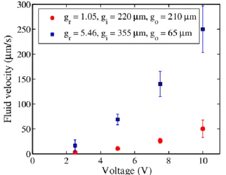
The understanding of alternating current electrothermal mechanism to control the open channel flow can be further elucidated by comparing the results for cases:

1.05( 220μm, 210μm)

r i o

g  g  g  and g_r 5.46 (g_i 355μm,g_o 65μm) shown in Fig. 7; parameters used in the simulation are conductivity 1.92 S/m and frequency 1 MHz. For g_r 1.05, the spacing of the electrodes along the channel is almost same and the

15

temperature gradient is almost uniform. Uniform temperature cannot generate variation in properties and thereby low electrothermal forces are induced. It is noteworthy that fluid velocity is much lower for g_r 1.05 in comparison with the case of g_r 5.46 at which the electrode spacing drastically changes from narrow gap to wider gap. Although the electrode gap gi 355μm is large compared to an electrode gap of gi 220 μm, where electric field strength is high (for gi 220 μm), steeper

temperature gradient prevailing in the fluid domain for gi 355μm results in higher fluid velocity. Therefore, tapering of the open channel plays a critical role to alter the flow velocity.

FIG. 7. Comparison of experimentally obtained fluid velocity for two different electrode arrangement:

1.05,5.46 r

g  . Parameters used in the experiment are: conductivity 1.92 S/m and frequency 1 MHz. Error bars are highlighted by the standard deviation. It is clear that value of error bar is the highest at relatively high voltage (= 10 V) due to fluctuation in the velocity values during experiments at 10 V.

IV. CONCLUSIONS

In summary, we demonstrate a novel strategy of generating directional free surface flow on a microfluidic chip, by deploying interactions between electrical forcing and strong local thermal gradients. Using the internally evoked Joule heating, spatially varying gradient in electrical conductivity and permittivity can be generated in the domain. Interactions between the gradients in electrical properties and the alternating voltage give rise to motion of mobile charges on the free surface of fluid, setting the fluid also into motion in a specific direction via interactions between electrical forces, buoyancy forcer and thermocapillary force. Our findings are likely to open up novel

16

research on efficient free-surface targeted transport for on-chip platforms used in biochemical analysis, without employing a geometrical confinement.

ACKNOWLEDGMENTS

This research has been supported by Indian Institute of Technology Kharagpur, India [Sanction Letter no.: IIT/SRIC/ATDC/CEM/2013-14/118, dated 19.12.2013]. SC acknowledges J. C. Bose National Fellowship awarded by the Department of Science and Technology, Government of India.

REFERENCES 1

V. Shankar and A. Sharma, “Instability of the interface between thin fluid films subjected to electric fields,” J. Colloid Interface Sci., 274, 294 (2004).

2

S. Qian, S.W. Joo, Y. Jiang, and M.A. Cheney, “Free-surface problems in electrokinetic micro- and nanofluidics,” Mech. Res. Commun., 36, 82 (2009).

3

M.A. André and P.M. Bardet, “Experimental study of shear layer instability below a free surface,” Phys. Fluids, 27, 112103 (2015).

4

J. Dhar, S. Mukherjee, S. Chakraborty, and others, “Universal oscillatory dynamics in capillary filling,” EPL (Europhysics Lett., 125, 14003 (2019).

5

W. Choi, A. Sharma, S. Qian, G. Lim, and S.W. Joo, “Is free surface free in micro-scale electrokinetic flows?,” J. Colloid Interface Sci., 347, 153 (2010).

6

S.W. Joo, “A new hydrodynamic instability in ultra-thin film flows induced by electro-osmosis,” J. Mech. Sci. Technol., 22, 382 (2008).

7

Y. Gao, T.N. Wong, C. Yang, and K.T. Ooi, “Two-fluid electroosmotic flow in microchannels,” J. Colloid Interface Sci., 284, 306 (2005).

8

U. Rosendahl, A. Grah, and M.E. Dreyer, “Convective dominated flows in open capillary channels,” Phys. Fluids, 22, 52102 (2010).

9

A.A. Kumar, B.J. Medhi, and A. Singh, “Experimental investigation of interface deformation in free surface flow of concentrated suspensions,” Phys. Fluids, 28, 113302 (2016).

10

Y. Temiz, R.D. Lovchik, G. V Kaigala, and E. Delamarche, “Lab-on-a-chip devices: How to close and plug the lab?,” Microelectron. Eng., 132, 156 (2015).

11

J. Gao, M.L.Y. Sin, T. Liu, V. Gau, J.C. Liao, and P.K. Wong, “Hybrid electrokinetic manipulation in high-conductivity media,” Lab Chip, 11, 1770 (2011).

12

G. Kunti, A. Bhattacharya, and S. Chakraborty, “Rapid mixing with high-throughput in a semi-active semi-passive micromixer,” Electrophoresis, 38, 1310 (2017).

13

T.M. Squires and M.Z. Bazant, “Induced-charge electro-osmosis,” J. Fluid Mech., 509, 217 (2004).

14

G. Kunti, A. Bhattacharya, and S. Chakraborty, “Numerical investigations of electrothermally actuated moving contact line dynamics: Effect of property contrasts,” Phys. Fluids, 29, 82009 (2017).

15

S. Chakraborty and S.K. Som, “Heat Transfer in an evaporating thin liquid film moving slowly along the walls of an inclined microchannel,” Int. J. Heat Mass Transf., 48, 2801 (2005).

16

17

viscoelastic fluids through concentric annulus,” RSC Adv., 6, 60117 (2016).

17

J. Dhar, U. Ghosh, and S. Chakraborty, “Electro-capillary effects in capillary filling dynamics of electrorheological fluids,” Soft Matter, 11, 6957 (2015).

18

E. Boyko, S. Rubin, A.D. Gat, and M. Bercovici, “Flow patterning in Hele-Shaw configurations using non-uniform electro- osmotic slip,” Phys. Fluids, 27, 102001 (2015).

19

C. Qi and C. Ng, “Electroosmotic flow of a two-layer fluid in a slit channel with gradually varying wall shape and zeta potential,” Int. J. Heat Mass Transf., 119, 52 (2018).

20

G. Kunti, A. Bhattacharya, and S. Chakraborty, “Alternating current electrothermal modulated moving contact line dynamics of immiscible binary fluids over patterned surfaces,” Soft Matter, 13, 6377 (2017).

21

G. Kunti, A. Bhattacharya, and S. Chakraborty, “Interfacial dynamics of immiscible binary fluids through ordered porous media: The interplay of thermal and electric fields,” Phys. Fluids, 31, 32002 (2019).

22

R. Chakraborty, R. Dey, and S. Chakraborty, “Thermal characteristics of electromagnetohydrodynamic flows in narrow channels with viscous dissipation and Joule heating under constant wall heat flux,” Int. J. Heat Mass Transf., 67, 1151 (2013).

23

S. Mandal, U. Ghosh, A. Bandopadhyay, and S. Chakraborty, “Electro-osmosis of superimposed fluids in the presence of modulated charged surfaces in narrow confinements,” J. Fluid Mech., 776, 390 (2015).

24

S. Chakraborty and S. Ray, “Mass flow-rate control through time periodic electro-osmotic flows in circular microchannels,” Phys. Fluids, 20, 83602 (2008).

25

M.Z. Bazant and T.M. Squires, “Induced-charge electrokinetic phenomena,” Curr. Opin. Colloid Interface Sci., 15, 203 (2010).

26

G. Kunti, P.K. Mondal, A. Bhattacharya, and S. Chakraborty, “Electrothermally modulated contact line dynamics of a binary fluid in a patterned fluidic environment,” Phys. Fluids, 30, 92005 (2018).

27

S. Talapatra and S. Chakraborty, “Double layer overlap in ac electroosmosis,” Eur. J. Mech., 27, 297 (2008).

28

W.Y. Ng, S. Goh, Y.C. Lam, C. Yang, and I. Rodríguez, “DC-biased AC-electroosmotic and AC-electrothermal flow mixing in microchannels,” Lab Chip, 9, 802 (2009).

29

G. Kunti, J. Dhar, S. Bandyopadhyay, A. Bhattacharya, and S. Chakraborty, “Energy-efficient generation of controlled vortices on low-voltage digital microfluidic platform,” Appl. Phys. Lett., 113, 124103 (2018).

30

J.J. Feng, S. Krishnamoorthy, and S. Sundaram, “Numerical analysis of mixing by electrothermal induced flow in microfluidic systems,” Biomicrofluidics, 1, 24102 (2007).

31

G. Kunti, A. Bhattacharya, and S. Chakraborty, “Analysis of micromixing of non-Newtonian fluids driven by alternating current electrothermal flow. Journal of Non-Newtonian Fluid Mechanics (Accepted article),” J. Nonnewton. Fluid Mech., (2017).

32

J.P. Urbanski, J.A. Levitan, D.N. Burch, T. Thorsen, and M.Z. Bazant, “The effect of step height on the performance of three-dimensional ac electro-osmotic microfluidic pumps,” J. Colloid Interface Sci., 309, 332 (2007).

33

E. Du and S. Manoochehri, “Microfluidic pumping optimization in microgrooved channels with ac electrothermal actuations,” Appl. Phys. Lett., 96, 34102 (2010).

34

A. Salari, M. Navi, and C. Dalton, “A novel alternating current multiple array electrothermal micropump for lab-on-a-chip applications,” Biomicrofluidics, 9, 14113 (2015).

35

Q. Lang, Y. Wu, Y. Ren, Y. Tao, L. Lei, and H. Jiang, “AC Electrothermal Circulatory Pumping Chip for Cell Culture,” ACS Appl. Mater. Interfaces, 7, 26792 (2015).

36

18

coplanar asymmetric electrode array,” Microfluid. Nanofluidics, 10, 521 (2011).

37

A. Kumar, S.J. Williams, H.-S. Chuang, N.G. Green, and S.T. Wereley, “Hybrid opto-electric manipulation in microfluidics—opportunities and challenges,” Lab Chip, 11, 2135 (2011).

38

Y. Ai, Z. Zeng, and S. Qian, “Direct numerical simulation of AC dielectrophoretic particle--particle interactive motions,” J. Colloid Interface Sci., 417, 72 (2014).

39

G. Kunti, J. Dhar, A. Bhattacharya, and S. Chakraborty, “Joule heating-induced particle manipulation on a microfluidic chip,” Biomicrofluidics, 13, 14113 (2019).

40

S.J. Williams, A. Kumar, and S.T. Wereley, “Electrokinetic patterning of colloidal particles with optical landscapes †,” Lab Chip, 1879 (2008).

41

S.J. Williams, A. Kumar, G. Green, and S.T. Wereley, “A simple , optically induced electrokinetic method to concentrate and pattern nanoparticles,” Nanoscale, 1, 133 (2009).

42

G. Kunti, A. Bhattacharya, and S. Chakraborty, “Alteration in contact line dynamics of fluid-fluid interfaces in narrow confinements through competition between thermocapillary and electrothermal effects,” Phys. Fluids, 30, 82005 (2018).

43

G. Kunti, J. Dhar, A. Bhattacharya, and S. Chakraborty, “Electro-thermally driven transport of a non-conducting fluid in a two-layer system for MEMS and biomedical applications,” J. Appl. Phys., 123, 244901 (2018).

44

J. Cao, P. Cheng, and F.J. Hong, “A numerical study of an electrothermal vortex enhanced micromixer,” Microfluid. Nanofluidics, 5, 13 (2008).

45

E. Du and S. Manoochehri, “Enhanced ac electrothermal fluidic pumping in microgrooved channels,” J. Appl. Phys., 104, 64902 (2008).

46

F.J. Hong, J. Cao, and P. Cheng, “A parametric study of AC electrothermal flow in microchannels with asymmetrical interdigitated electrodes,” Int. Commun. Heat Mass Transf., 38, 275 (2011).

47

F.J. Hong, F. Bai, and P. Cheng, “Numerical simulation of AC electrothermal micropump using a fully coupled model,” Microfluid. Nanofluidics, 13, 411 (2012).

48

V. Studer, A. Pepin, Y. Chen, and A. Ajdari, “An integrated AC electrokinetic pump in a microfluidic loop for fast and tunable flow control.,” Analyst, 129, 944 (2004).

49

M. Zehavi, A. Boymelgreen, and G. Yossifon, “Competition between Induced-Charge Electro-Osmosis and Electrothermal Effects at Low Frequencies around a Weakly Polarizable Microchannel Corner,” Phys. Rev. Appl., 5, 44013 (2016).

50

K. Yang and J. Wu, “Investigation of microflow reversal by ac electrokinetics in orthogonal electrodes for micropump design,” Biomicrofluidics, 2, 24101 (2008).

51

P. García-Sánchez, A. Ramos, and F. Mugele, “Electrothermally driven flows in ac electrowetting,” Phys. Rev. E, 81, 15303 (2010).

52

Q. Lang, Y. Ren, D. Hobson, Y. Tao, L. Hou, Y. Jia, Q. Hu, J. Liu, X. Zhao, and H. Jiang, “In-plane microvortices micromixer-based AC electrothermal for testing drug induced death of tumor cells,” Biomicrofluidics, 10, 64102 (2016).

53

J. Wu, M. Lian, and K. Yang, “Micropumping of biofluids by alternating current electrothermal effects,” Appl. Phys. Lett., 90, 234103 (2007).

54

S.J. Williams and N.G. Green, “Electrothermal pumping with interdigitated electrodes and resistive heaters,” Electrophoresis, 36, 1681 (2015).

55

G. Kunti, A. Bhattacharya, and S. Chakraborty, “Electrothermally actuated moving contact line dynamics over chemically patterned surfaces with resistive heaters,” Phys. Fluids, 30, 62004 (2018).

56

M. Lian and J. Wu, “Ultrafast micropumping by biased alternating current electrokinetics,” Appl. Phys. Lett., 94, 64101 (2009).

57

19 Studies Press, Philadelphia, 2003).

58

A. Ramos, Electrokinetics and Electrohydrodynamics in Microsystems (Springer, New York, 2011).

59

Castellanos A, Electrohydrodynamics (Springer, New York, 1998).

60

D.R. Lide, CRC Handbook of Chemistry and Physics, 84th ed. (CRC Press, London, 2003).

61

A. Ramos, H. Morgan, N.G. Green, and A. Castellanos, “Ac electrokinetics: a review of forces in microelectrode structures,” J. Phys. D. Appl. Phys., 31, 2338 (1998).

62

N.G. Green, A. Ramos, A. Gonzalez, A. Castellanos, and H. Morgan, “Electrothermally induced fluid flow on microelectrodes,” J. Electrostat., 53, 71 (2001).

63

A. Castellanos, A. Ramos, A. González, N.G. Green, and H. Morgan, “Electrohydrodynamics and dielectrophoresis in microsystems: scaling laws,” J. Phys. D. Appl. Phys., 36, 2584 (2003).

64

M. Sigurdson, D. Wang, and C.D. Meinhart, “Electrothermal stirring for heterogeneous immunoassays,” Lab Chip, 5, 1366 (2005).

65

H.C. Feldman, M. Sigurdson, and C.D. Meinhart, “AC electrothermal enhancement of heterogeneous assays in microfluidics,” Lab Chip, 7, 1553 (2007).

66

H. Liu, A.J. Valocchi, Y. Zhang, and Q. Kang, “Phase-field-based lattice Boltzmann finite-difference model for simulating thermocapillary flows,” Phys. Rev. E, 87, 13010 (2013).

67

H. Liu, A.J. Valocchi, Y. Zhang, and Q. Kang, “Lattice Boltzmann phase-field modeling of thermocapillary flows in a confined microchannel,” J. Comput. Phys., 256, 334 (2014).

68

D. Jacqmin, “Contact-line dynamics of a diffuse fluid interface,” J. Fluid Mech., 402, 57 (2000).