HAL Id: hal-02625146
https://hal.archives-ouvertes.fr/hal-02625146
Submitted on 2 Jul 2020
HAL is a multi-disciplinary open access
archive for the deposit and dissemination of
sci-entific research documents, whether they are
pub-lished or not. The documents may come from
teaching and research institutions in France or
abroad, or from public or private research centers.
L’archive ouverte pluridisciplinaire HAL, est
destinée au dépôt et à la diffusion de documents
scientifiques de niveau recherche, publiés ou non,
émanant des établissements d’enseignement et de
recherche français ou étrangers, des laboratoires
publics ou privés.
LMDZ-NEMO-med-V1, to conduct global-to-regional
past climate simulation for the Mediterranean basin: an
Early Holocene case study
Tristan Vadsaria, Laurent Li, Gilles Ramstein, Jean-Claude Dutay
To cite this version:
Tristan Vadsaria, Laurent Li, Gilles Ramstein, Jean-Claude Dutay. Development of a sequential tool,
LMDZ-NEMO-med-V1, to conduct global-to-regional past climate simulation for the Mediterranean
basin: an Early Holocene case study. Geoscientific Model Development, European Geosciences Union,
2020, 13 (5), pp.2337-2354. �10.5194/gmd-13-2337-2020�. �hal-02625146�
https://doi.org/10.5194/gmd-13-2337-2020 © Author(s) 2020. This work is distributed under the Creative Commons Attribution 4.0 License.
Development of a sequential tool, LMDZ-NEMO-med-V1, to
conduct global-to-regional past climate simulation for the
Mediterranean basin: an Early Holocene case study
Tristan Vadsaria1,3, Laurent Li2, Gilles Ramstein1, and Jean-Claude Dutay1
1Laboratoire des Sciences du Climat et de l’Environnement, CEA-CNRS- Université Paris Saclay,
Gif-sur-Yvette, France
2Laboratoire de Météorologie Dynamique, CNRS-ENS-Ecole Polytechnique Sorbonne Université, Paris, France 3Atmosphere and Ocean Research Institute, the University of Tokyo, Kashiwa, Chiba, Japan
Correspondence: Tristan Vadsaria ([email protected], [email protected])
Received: 19 July 2019 – Discussion started: 30 August 2019
Revised: 29 February 2020 – Accepted: 6 April 2020 – Published: 19 May 2020
Abstract. Recently, major progress has been made in the simulation of the ocean dynamics of the Mediterranean using atmospheric and oceanic models with high spatial resolution. High resolution is essential to accurately capture the synoptic variability required to initiate intermediate- and deep-water formation, the engine of the Mediterranean thermohaline cir-culation (MTC). In paleoclimate studies, one major prob-lem with the simulation of regional climate changes is that boundary conditions are not available from observations or data reconstruction to drive high-resolution regional models. One consistent way to advance paleoclimate modelling is to use a comprehensive global-to-regional approach. However, this approach needs long-term integration to reach equilib-rium (hundreds of years), implying enormous computational resources. To tackle this issue, a sequential architecture of a global–regional modelling platform has been developed for the first time and is described in detail in this paper. First of all, the platform is validated for the historical period. It is then used to investigate the climate and in particular, the oceanic circulation, during the Early Holocene. This period was characterised by a large reorganisation of the MTC that strongly affected oxygen supply to the intermediate and deep waters, which ultimately led to an anoxic crisis (called sapro-pel). Beyond the case study shown here, this platform may be applied to a large number of paleoclimate contexts from the Quaternary to the Pliocene, as long as regional tectonics re-main mostly unchanged. For example, the climate responses of the Mediterranean basin during the last interglacial
pe-riod (LIG), the Last Glacial Maximum (LGM) and the Late Pliocene all present interesting scientific challenges which may be addressed using this numerical platform.
1 Framework of the study
1.1 Introduction
The Mediterranean basin is a key region for the global cli-mate system. It is considered to be a clicli-mate “hotspot” (Giorgi, 2006) due to its high sensitivity to global warming. In the past, it has been the seat of important human civil-isations, and it continues to play a very important role in international geopolitics with a dense population along its coasts. There is great diversity in the Mediterranean ecosys-tems, both marine and terrestrial. The Mediterranean region is also rich in paleoclimate records with a variety of prox-ies. Indeed, this area experienced major changes during the glacial–interglacial cycles (Jost et al., 2005; Ludwig et al., 2018; Ramstein et al., 2007). Another long-term cycle of changes due to high-frequency precession which drastically modified the hydrological patterns of this area (monsoon, sapropels) is also superimposed.
Due to the peculiarities of both the atmospheric and oceanic circulation in the region, high-quality climate mod-elling of the Mediterranean region needs to have high spatial resolution (Li et al., 2006). Indeed, the presence of strong
gusts of wind in winter is essential to trigger oceanic con-vection, and these can only be correctly represented in high-resolution models. Limited area models (LAMs), or regional climate models (RCMs), present some advantages in this re-gard, since they generally demand less computing resources, allowing them to be run at high spatial resolution for a given region. However, their usefulness for paleoclimate purposes is limited because of the lack of adequate lateral boundary conditions to drive the RCMs. The main reason why few comprehensive modelling exercises to explain paleoclimate changes around the Mediterranean have been performed is that the level of computing resources required for high reso-lution and long simulations is inaccessible. This is especially true in the case of the Mediterranean thermohaline circula-tion (MTC), which has significantly changed in the past, at both centennial and millennial scales.
Here, we describe a modelling suite to define high-resolution atmospheric conditions over the Mediterranean basin from global Earth system model (ESM) paleoclimate simulations. This atmospheric forcing can then be used to run a highly resolved ocean model (NEMOMED8 1/8◦) to accurately simulate ocean dynamics. This tool allows us to achieve a high spatial resolution and equilibrated simulations with a runtime of 100 years. The objective of this study is to develop a modelling platform sufficiently comprehensive to conduct paleoclimate studies of the Mediterranean basin. The potential of this platform is illustrated by investigating climate situations from the present period and from the Early Holocene which is supposed to generate sapropel events.
The sapropel events provide excellent case studies on the impact of global changes on the Mediterranean basin. These periodic events are related to a long period of anoxia of the deep and bottom waters triggered by an enhancement of the African monsoon caused by periodicities of the orbital precession. However, the localisation of the forcing source caused by orbital variability is still a subject of debate. This is especially true for the last sapropel, denoted S1, which occurred during the Early Holocene (between 10 500 and 6800 BP) (De Lange et al., 2008). Reproducing past climate variations over the Mediterranean basin, including the sapro-pel events, is therefore a challenge for the modelling com-munity.
The paper is organised as follows. In the first section, we briefly review the different approaches used to simulate the Mediterranean climate and sea conditions, and we also present the concept of the sequential procedure that we pro-pose. Section 2 presents in detail the model architecture we developed. Finally, we present applications with simulations of the historical period (1970–1999) in Sect. 3 and the Early Holocene (around 9.5 ka) in Sect. 4.
1.2 Overview of current Mediterranean Sea modelling
The Mediterranean Sea, due to its limited size and its semi-enclosed configuration, has a faster equilibrium response
(102years) than the global ocean (103years). Because of this semi-enclosed configuration, there are a few requirements that modelling of the Mediterranean Sea needs to satisfy so that its evolution can be properly represented. High resolu-tion in both the atmospheric forcing and the oceanic config-uration is necessary to correctly simulate the convection ar-eas and the associated thermohaline circulation (Lebeaupin Brossier et al., 2011; Li et al., 2006). Depending on the mech-anism studied, the resolution of the ocean model used by the research community ranges from 1/4◦(e.g. for paleoclimatic simulation) to 1/75◦ (for hourly description of the mixed-layer, tide-based investigation). The results for oceanic con-vection are highly dependent on the flux of heat, flux of wa-ter and the wind stress at the air–sea inwa-terface, especially the seasonal variability and intensity. There are many modelling configurations in the scientific literature, making it impossi-ble to provide an exhaustive review of all of them. We can summarise them by presenting the different approaches used to drive the Mediterranean oceanic model, along with their advantages and drawbacks. We underline our new, coherent method, which captures the changes in ocean dynamics in the Mediterranean basin derived from global paleoclimate simu-lations.
1.2.1 Observations and reanalysis
The most common way to simulate the general circulation of the Mediterranean Sea is to run a regional oceanic gen-eral circulation model forced by surface fluxes and wind stresses derived from observations and reanalyses. In this way, an oceanic model can be driven by realistic fluxes. In most cases, this implies an observation-based reconstruction of relevant variables with a spatial atmospheric resolution of less than 50 km and a daily temporal resolution, at a mini-mum, in order to simulate the formation of dense water (Ar-tale, 2002). This approach is adapted to simulate the present-day Mediterranean Sea and to explore the complexity of its sub-basin circulation and water mass formation (Millot and Taupier-Letage, 2005). However, it is not well adapted to the study of past and future climate, partly due to the excessive computing resources needed.
1.2.2 Atmospheric model
A second method consists of forcing a regional oceanic model with simulations from an atmospheric model, AGCM (atmospheric global climate model) or ARCM (atmospheric regional climate model). Since the AGCM resolution (typi-cally 100 to 300 km horizontally) is coarse, statistical and/or dynamical downscaling is usually needed, especially for wind stress so that the ORCM (ocean regional circulation model) can be correctly forced (Béranger et al., 2010). Cur-rently, dynamical downscaling with ARCM is the preferred option because it generally improves simulations of the
cli-mate in the Mediterranean region and especially of the hy-drological cycle (Li et al., 2012).
This configuration is broadly used to assess anthropogenic climate changes (Adloff et al., 2015; Macias et al., 2015; Somot et al., 2006). In these studies, the Mediterranean Sea simulations are generally driven by the outputs of an ARCM, which is, in turn, driven by the global climate model (GCM) or observation-based reanalysis. It should be noted that bi-ases in oceanic variables can be reduced through constant flux correction (Somot et al., 2006). This configuration is suitable for high-resolution simulation of the past Mediter-ranean Sea (Mikolajewicz, 2011, for the Last Glacial Max-imum (LGM); Adloff et al., 2011, for the Early Holocene, among others).
1.2.3 Regional coupled model
Although the majority of the Mediterranean Sea models are ocean-alone models, some of them use a coupled configu-ration between the Mediterranean Sea and the atmosphere. Such a coupled configuration generally improves the simu-lation of the air–sea fluxes, including their annual cycle (De Zolt et al., 2003), but may show climate drifts in key parame-ters such as the sea surface temperature (SST). Regional cou-pled models are now emerging as a tool in Mediterranean cli-mate modelling (Artale et al., 2010; Dell’Aquila et al., 2012; Drobinski et al., 2012; Sevault et al., 2014; Somot et al., 2008). However, this full-coupling configuration is currently not possible for high-resolution paleoclimate issues requiring long simulation for hundreds or thousands of years.
1.2.4 Importance of boundary conditions
The boundary conditions applied to the Mediterranean Sea domain, in particular, the exchanges of water, salt and heat with the Atlantic Ocean through the Strait of Gibraltar, sig-nificantly modulate the Mediterranean circulation (Adloff et al., 2015). This is especially true at the millennial scale where deglaciation episodes and fluctuations of the AMOC (At-lantic Meridional Overturning Circulation) and the Mediter-ranean Sea affect each other (Swingedouw et al., 2019). The level of discharge from the main rivers is also crucial as is illustrated by the sapropel episodes, where an increase in freshwater input drastically slowed down the MTC. Most of current models impose prescribed (observed when possible) conditions in the near-Atlantic zone, including temperature and salinity. The same methodology can be used to prescribe river discharges. However, it must be acknowledged that de-termining inputs from rivers into the Mediterranean Sea, ei-ther of water or oei-ther materials, still presents serious chal-lenges for modelling.
1.3 Concepts for a sequential procedure to perform global-to-regional modelling
In this paper, a new architecture for high-resolution mod-elling of the climate of the Mediterranean basin for past, present and future conditions is proposed. This architecture is based on a method that provides as much compatibility as possible amongst the models used and high consistency with data.
1.3.1 Step 1: global climate
Our goal is to simulate different climate conditions for the Mediterranean basin. The first step of any relevant proce-dure should be to simulate the global climate conditions from which the simulation of the regional climate is driven. These may be already available in simulations from previous Paleo-climate Modelling Intercomparison Project (PMIP) exercises for various periods (e.g. mid-Holocene, Last Glacial Maxi-mum, last interglacial and mid-Pliocene) as well as for dif-ferent sapropel events and interglacials (e.g. MIS11, MIS13 and MIS19). However, this is not always possible due to the large volume of high-frequency 3-D atmospheric circulation variables involved. An alternative approach, used in some re-gional climate simulations (Chen et al., 2011; Goubanova and Li, 2007; Krinner et al., 2014), consists of using an AGCM (either an independent one or the same one used for the global climate simulation) run with appropriate values for global SST and sea-ice cover (SIC), derived from PMIP global simulations. SST is crucial to determine atmospheric features and responses, while SIC plays a key role in deter-mining the global albedo. Monthly SST and SIC are neces-sary and sufficient to drive an AGCM. They can be acquired from global climate simulations or through a bias-correction procedure.
1.3.2 Step 2: regional climate
After running an AGCM, regional climate can be now repro-duced with an ARCM nested into the high-frequency out-puts from the AGCM. Of course, the ARCM can be run in parallel to the AGCM or with a small time delay. Thus, we avoid a large accumulation of intermediate information be-tween the AGCM and the ARCM. In our study, we assume that there would be no feedback from the regional scale to the global scale, so only a “one-way” transfer of information (from global to regional scale) is considered. In our case, the ARCM is a strongly zoomed-in version of the AGCM and is also driven by monthly SST and SIC values, as used for AGCM. The higher resolution of the ARCM allows the syn-optic variability and seasonality of the Mediterranean region to be depicted so that a realistic wind pattern and hydrologi-cal cycle may be reproduced. This approach provides a gen-eral framework for use in many different paleoclimate
peri-ods from the Pliocene to the Pleistocene, as long as the basin tectonics remain unchanged.
1.3.3 Step 3: Mediterranean Sea circulation
Daily air–sea fluxes and wind stress provided by the ARCM are used as surface boundary conditions to drive the ORCM to investigate the oceanic dynamics of the Mediterranean. It is reasonable to assume that the boundary conditions of these air–sea fluxes represent the long-term trends of the oceanic dynamics. Rivers may be considered interactive or not de-pending on the investigative objectives: runoff can be pre-scribed from climatology or obtained from the hydrologi-cal component of the surface model. Again, we highlight that our architecture does not include any feedback, between either the regional ocean and the regional atmosphere, or the regional ocean and the global ocean. This configuration means that we can avoid dealing with certain issues, for ex-ample, the influence of the Mediterranean outflow water on the North Atlantic Ocean, but it is well adapted to provide consistent river runoff associated with changes in continen-tal precipitation.
2 Model architecture
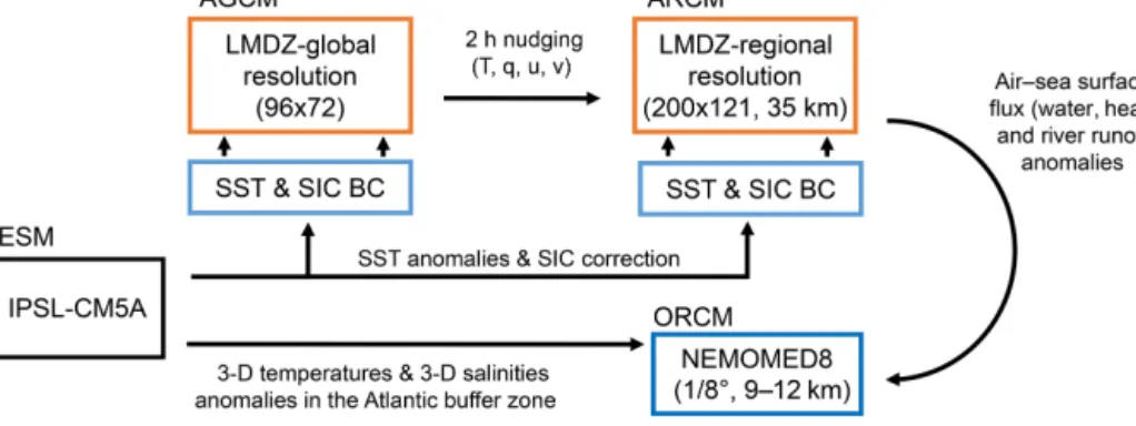
An ensemble of modelling tools that includes two atmo-spheric models and a regional oceanic model is used. Fig-ure 1 summarises the configuration and shows the experi-mental flowchart.
2.1 The atmospheric models (AGCM and ARCM)
LMDZ4 (Hourdin et al., 2006; Li, 1999) is the atmospheric general circulation model developed and maintained by IPSL (Institut Pierre Simon Laplace). It has been widely used in previous phases of Coupled Model Intercomparison Project (CMIP) and PMIP projects. The resolution of the model is variable. Its global version used here (referred to as LMDZ4-global) is 3.75◦in longitude and 2.5◦in latitude with 19 lay-ers in the vertical. It provides the boundary conditions to drive LMDZ4-regional. LMDZ4-regional (Li et al., 2012) is a regionally oriented version of LMDZ4 with the same physics and same vertical discretisation, dedicated to the Mediterranean region. The zoomed-in model covers an ef-fective domain of 24 to 56◦N and 13◦W to 43◦E, with a horizontal resolution of about 30 km inside the zoom. The rest of the globe outside this domain is considered to be the buffer zone for LMDZ4-regional where a relaxation opera-tion is performed to nudge the model with variables from the AGCM at a 2 h frequency. The resolution of LMDZ4-regional decreases rapidly outside its effective domain. In both LMDZ4-global and LMDZ4-regional, land-surface pro-cesses, including the hydrological cycle, are taken into ac-count through a full coupling with the surface model,
Organ-ising Carbon and Hydrology In Dynamic Ecosystems (OR-CHIDEE) (Krinner et al., 2005).
2.2 The regional oceanic model (ORCM)
NEMOMED8 (Beuvier et al., 2010; Herrmann et al., 2010) is the regional Mediterranean configuration of the Nucleus for European Modelling of the Ocean (NEMO) oceanic mod-elling platform (Madec, 2008). The horizontal domain in-cludes the Mediterranean Sea and the nearby Atlantic Ocean, which serves as a buffer zone (from 11 to 7.5◦W). The hor-izontal resolution is 1/8◦in longitude and 1/8◦cos ϕ in lat-itude, i.e. 9 to 12 km from the north to the south. The model has 43 layers of inhomogeneous thickness (from 7 m at the surface to 200 m in the depths) in the vertical. River dis-charges are accounted for as freshwater fluxes in the grids corresponding to the river mouths. A dataset of climatologi-cal river discharges was proposed by default to cover the en-tire Mediterranean draining basin with 33 river mouths. It is of course switched off when rivers are interactive in the plat-form. The interactive calculation of freshwater discharges from rivers by the land-surface model (ORCHIDEE) in-cludes 192 river mouths that cover the Mediterranean drain-ing basin. The Black Sea, not included in NEMOMED8, counts as a river dumping freshwater into the Aegean. The deposit rate is calculated based on total runoff into the Black Sea, plus the net budget of precipitation (P ) minus evapora-tion (E) over the Black Sea.
When the oceanic model NEMO is used alone, with prescribed surface fluxes, it is indispensable to imple-ment a restoring term with a constant coefficient of 40 W m−2K−1(as defined in Barnier et al., 1995). This is a standard procedure for NEMO to prevent eventual runaway cases. In our modelling chain, the target temperature for the restoration is the surface air temperature from the regional atmospheric model (LMDZ4-regional).
2.3 Modelling sequence
As shown in Fig. 1, the first step in our modelling chain is to obtain SST and SIC values from an Earth system model simulation able to reproduce global climate (for the past, present or future). We can reasonably hypothesise that ma-jor global climate information can transit from global SST and SIC. This hypothesis was deemed legitimate for climate downscaling purposes for Antarctic and Africa, in Krinner et al. (2014) and Hernández-Díaz et al. (2017), respectively. In the present work, we use IPSL-CM5A (Dufresne et al., 2013) to extract relevant SST and SIC values to drive the AGCM (LMDZ4-global) and the ARCM (LMDZ4-regional). The next step is to run the two atmospheric models (LMDZ4-global and LMDZ4-regional) in the usual way, as proposed by the Atmospheric Model Intercomparison Project (AMIP) community. This is the most expensive step, as atmospheric models are the most demanding in terms of computing
re-Figure 1. Flowchart of the modelling chain including the four main components generally represented by ESM, AGCM, ARCM and ORCM, respectively, and actually implemented in our platform by IPSL-CM5A, LMDZ-global, LMDZ-regional and NEMOMED8. BC: boundary condition, u: zonal wind, v: meridional wind, q: specific humidity, T : temperature, S: salinity, SST: sea surface temperature, SIC: sea-ice concentration.
sources. Fortunately, it is not necessary to run them for a long time as the atmosphere reaches equilibrium quickly. We ap-plied 30 years of simulation to both models. We consider this duration to be long enough to depict climate variability for the simulation of past events. The AGCM nudges the ARCM in the conventional way of one-way nesting for temperature, humidity, meridional and zonal wind every 2 h. The nudg-ing is done usnudg-ing an exponential relaxation procedure with a timescale of half an hour outside the zoom and 10 d inside the zoom. Table S2 in the Supplement summarises the forcings used, especially the orbital forcing and atmospheric CO2.
The necessary variables (surface air temperature, wind stress, P –E over the sea, heat fluxes) are provided by ARCM to NEMOMED8 (ORCM) at daily frequency. The salinity and temperature conditions are provided in three dimensions in the Atlantic buffer zone, near the Strait of Gibraltar, and updated every month. River runoff, updated every month, de-pends on the configuration used (prescribed climatological rivers or interactive rivers). Table S3 in SOM details these boundary conditions.
It is worthy to mention the work of Mikolajewicz (2011), who used a similar modelling chain (from a coarse-resolution Earth system model to a high-resolution regional oceanic model) to simulate the Mediterranean Sea climate during the Last Glacial Maximum. However, Mikolajewicz (2011) used only an AGCM (ECHAM5) as the intermediate step. In our case, we found that the use of ARCM was indispens-able to produce high-quality forcing to correctly simulate the oceanic convection in NEMOMED8.
2.4 Bias correction
The sequential modelling chain, despite the lack of interac-tivity and feedback at interfaces, allows for error removal and bias correction at each step of the methodology. This adjust-ment is sometimes crucial, especially when model outputs need to be of very high quality to be incorporated into im-pact studies. This concept was further described in Krinner et
al. (2019), as illustrated in Fig. 16 of their paper. Therefore, to enhance our confidence in the realism of the simulation results, bias correction may be introduced when necessary. The correction method used in the present work generally follows the conventional procedure, which is based on the difference between the model outputs for present-day simu-lations and actual observations. Biases corrected in this way, theoretically only valid for the historical simulation (named HIST hereafter), are assumed to remain unchanged for past and future simulation scenarios. However, the transferabil-ity between past and future periods is questionable. There is no guarantee that the model error for one period is the same for other periods, even though the model physics may be the same. In addition, paleodata are often rare and incom-plete, and thus are unsuitable for evaluation and correction of model errors. The most reliable basis is that established for the present day. The reader can find a full description of the bias corrections and their eventual use in our applications in the Supplement (Sect. S2: bias correction).
3 Validation of the modelling chain for present-day climate 1970–1999
In this section, the capacity of the model to reproduce the cli-mate of the recent past is evaluated, in particular, its ability to simulate sea surface characteristics as well as the mixed-layer depth (MLD) and oceanic convection patterns as these are key elements to reproduce the evolution of the Mediter-ranean Sea in past climate conditions.
3.1 Experimental design
For the HIST experiment, SST and SIC observations (ERA-Interim; Dee et al., 2011) are used to force the AGCM. River runoff is from the climatology of Ludwig et al. (2009). Monthly mean climatological sea temperatures and salinities (World Ocean Atlas database from Locarnini et al., 2013; Zweng et al., 2013) are used for the Atlantic boundary zone.
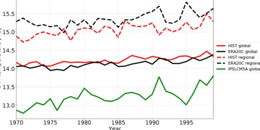
Figure 2. Time series of annual mean surface air temperatures at 2 m in HIST (red) and ERA20C (black; Stickler et al., 2014) and IPSL-CM5A (green) for the global average (solid lines) and Mediterranean region (20–50◦N, 10◦W–35◦E) average (dashed lines).
Figure 3. Annual mean precipitation, (a) meridionally averaged (30 to 50◦N), (b) zonally averaged (−10 to 35◦E), in the historical sim-ulations with an AGCM (LMDZ-global) and ARCM (LMDZ-regional). Observation comes from GPCP (Global Precipitation Climatology Project, 1979 to 1999, blue line; Adler et al., 2018) and ERA-20C (green line; Stickler et al., 2014).
HIST atmospheric simulations for both global and regional simulations have a duration of 30 years. The length of the HIST oceanic simulation is also 30 years but obtained after a 150-year spinup. The forcings for each experiment are de-tailed in Tables S2 and S3 in the Supplement. Spinup phases for each simulation are also shown from Figs. S4 to S8 for the overturning stream function and the index of stratification.
3.2 Evolution of temperatures
Figure 2 depicts the temporal evolution, between 1970 and 1999, of annual mean surface air temperatures at 2 m in the atmospheric simulations (global and regional) compared to observations for the whole globe and over the Mediterranean
region. The two models reproduce a range of temperatures similar to the observations, with the Mediterranean tempera-tures warmer than the global temperatempera-tures. The global simu-lation (continued red curve in Fig. 2), after SST bias correc-tion, is very close to the observation (continued black curve), with a tremendous improvement compared to IPSL-CM5A (green curve in Fig. 2) The regional model reproduces the warming trend and aspects of the interannual variability close to observations but with a mean cold shift of about −0.6◦C.
3.3 Precipitation and freshwater budget
Figure 3a and b show the average annual precipitation for 1970–1999 in HIST over the Mediterranean region and the
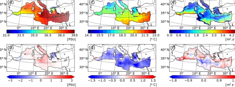
Figure 4. Annual mean sea surface salinity (SSS) (a, b, in PSU), sea surface temperature (c, d, in◦C) and index of water column stratification (e, f, winter IS in m2s−2) simulated in HIST (a, c, e) and the HIST deviation (model–obs) from the observation-based MEDATLAS data (averaged over the entire simulation).
differences with observations. The main features of the dis-tribution of precipitation over the Mediterranean region are simulated, in particular the distinct contrast between the very low precipitation in the southern region and higher precip-itation in the north. The ARCM tends to generate higher precipitation than the AGCM due to the resolution refine-ment. Compared to observation, AGCM is closer to ERA20C (Stickler et al., 2014), whereas ARCM is closer to GPCP data (Adler et al., 2018). However, the regional model still over-estimates the amount of precipitation, especially at 42◦N, from 45 to 50◦N, at 8 and 20◦E. It corresponds to most of Europe, especially over the Alps, the Pyrenees, the Balkans and other mountainous regions. The freshwater budget over the Mediterranean Sea from observations (a synthesis from Sanchez-Gomez et al., 2011, and from other sources) and in the various simulations conducted in this study are summed up in Table 1. The simulated continental precipitation is over-estimated, but both the precipitation and evaporation over the Mediterranean Sea in HIST are very close to the observa-tions. The two other simulations included in Table 1 (PIC-TRL and EHOL) are those designed to investigates the Early Holocene climate (see Sect. 4).
3.4 Mediterranean Sea surface characteristics
Figure 4 displays the temperatures and salinities of the Mediterranean Sea simulated in HIST and the deviations from observations. The model is able to capture the main characteristics of the pronounced west–east gradient of sea surface salinity (SSS) in the Mediterranean Sea (Fig. 4a). Values are within the range of observations (mean bias of 0.32 PSU, error of 0.37 PSU, Table 2). In the simulation, the Aegean Sea is not salty enough (about −1.5 PSU) and the Adriatic/Ionian Sea is too salty (+1 PSU).
The model reproduced the northwest to southeast tempera-ture gradient, as shown in Fig. 4b. However, the model shows a general cold bias (from −0.5 to −1.5◦C) over the entire Mediterranean (Fig. 4e), due to the cold bias already ob-served for the air temperature at 2 m in the regional atmo-spheric forcing (cf. Fig. 2).
3.5 Mediterranean thermohaline circulation
Here, the general characteristics of the simulated thermoha-line circulation is evaluated in regions where deep and inter-mediate water formation occurs. Figure 4c displays the strat-ification index (IS1) for HIST. IS is a vertical integration of the Brunt–Väisälä frequency. A lower IS implies that convec-tion is more likely. The range of IS biases (Fig. 4f) is from −1 to 1 m2s−2(mean bias of 0.91 m2s−2, error of 0.29 m2s−2). The model satisfactorily reproduces the convection in known intermediate- and deep-water formation areas, namely the Gulf of Lion, the Adriatic Sea, the Ionian Sea, the Aegean Sea and the northern Levantine.
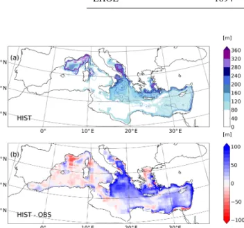
Comparison with observations of the mixed-layer depth (Houpert et al., 2015) confirms that the model reproduces re-alistic intermediate- and deep-water formation patterns, with a thicker MLD in the eastern basin, due to salty conditions (Fig. 4a and e), and a shallower MLD in the Gulf of Lion (Fig. 5b).
The simulated Mediterranean overturning circulation is analysed (Fig. 6). The zonal overturning stream function
1IS(x, y, h) =Rh
0N2(x, y) zdz. N2 is the Brunt–Väisälä
fre-quency. IS is calculated at each model grid (x, y) for a given depth h (set as the bottom of the sea or as 1000 m when the depth is greater than 1000 m).
Table 1. The Mediterranean Sea freshwater budget, expressed as mm yr−1for the whole water area (about 2.5 million km2). E is evaporation; P is precipitation; R is river runoff; B is Black Sea discharge into the Mediterranean Sea. OBS is a summary from Sanchez-Gomez et al. (2011) for P , E and P –E, from Ludwig et al. (2009) for R, from Lacombe and Tchernia (1972), Stanev et al. (2000) and Kourafalou and Barbopoulos (2003) for B. River discharges in HIST are from the climatology of Ludwig et al., (2009). PICTRL uses the Nile of its pre-industrial (pre-damming) value (2930 m3s−1) annually (Rivdis database; Vorosmarty et al., 1998). River discharges in EHOL are deduced from the difference between EHOL and PICTRL.
Dataset or experiment E P R B E–P –R–B OBS 1096–1136 256–595 102–142 73–121 238–705
HIST 1106 443 74 104 485
PICTRL 1031 451 98 104 378
EHOL 1094 460 225 104 305
Figure 5. (a) Mixed-layer depth simulated in HIST (m) and as a deviation (b) of HIST from observations of Houpert et al. (2015) averaged over the entire simulation for JFM (January–February– March). Contour lines in panel (a) represent the maximum of MLD throughout the HIST simulation.
(ZOF2) in Fig. 6a depicts the surface and intermediate cir-culation and the intermediate/deep circir-culation. The surface current from the Strait of Gibraltar flows up to 30◦E and back to the Atlantic Ocean in the intermediate layers, through the Levantine intermediate water (LIW) outflow. Figure 6c, e and g represent the meridional overturning stream function (MOF3) in the Gulf of Lion, the Adriatic Sea and the Aegean Sea, respectively. The surface cell in the longitude–depth plan is comparable to previous studies done with the same regional oceanic model but with different forcings (Adloff et al., 2015; Somot et al., 2006): the mean strength of the surface cell ranges from 0.8 to 1.0 Sv, and the longitudinal
2ZOF(x, z) =Rz h
Ryn
ysu(x, y, z)dydz. u is the zonal currents, h is
the depth of the bottom, ynand ysare the north and south
coordi-nates, respectively.
3MOF(y, z) =Rz
h
Rxw
xe v(x, y, z)dxdz. v is the meridional
cur-rents, h is the depth of the bottom, xwand xeare the west and east
coordinates, respectively.
extension is from 5◦W to 30◦E. The simulated intermediate and deep cells are recognised in existing studies as having different characteristics. Our simulated pattern is very close to a similar historical run in Adloff et al. (2015) but is weaker than a historical run in Somot et al. (2006) and a second his-torical configuration (with refined air–sea flux) in Adloff et al. (2015). The ZOF in HIST depicted in Fig. 6) is consis-tent with the reanalyses (1987–2013) of Pinardi et al. (2019) over the western basin but shows a weaker eastern deep cell compared to the reconstruction.
3.6 Summary of validation
Validation of our platform was based on the historical period (1970 to 1999). The atmospheric simulation is acceptable compared with observations for the air temperature at 2 m at both global and regional scales. The simulated precipita-tion from the atmospheric models produces a signal that has the same range of variability as the observations, but there is significant overestimation of precipitation over the moun-tainous area and over the land surrounding the Mediterranean Sea. However, the freshwater budget over the sea is close to observations for both evaporation and precipitation. The areas of intermediate and deep convection produced by the model are realistic, and the simulation of the thermohaline circulation is well captured by the oceanic model and in the range of the state-of-the-art existing Mediterranean regional models (compared to the simulations of Adloff et al., 2015, and Somot et al., 2006, for instance) and reanalysis as well (Pinardi et al., 2019). These features inspire confidence in our modelling platform for the investigations of past climate.
4 Application of the modelling chain to the Early Holocene
In this section, results obtained when our sequential mod-elling chain is applied in a paleoclimate context are pre-sented, which was our initial motivation for developing this modelling tool. We chose to test the performance of our tool on the Early Holocene, a period marked by significant changes in climate and ocean dynamics over the
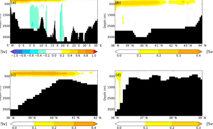
Mediter-Figure 6. (a, b) Zonal overturning stream function (ZOF) integrated from north to south and shown as a longitude–depth section for the whole Mediterranean Sea, for the HIST and PICTRL simulations (from top to bottom), respectively. Other panels show meridional overturning stream function (MOF) shown as a latitude–depth section, integrated west/east for the Gulf of Lion (c, d, longitudinal extent: 4.5–8◦E), the Adriatic/Ionian Sea (e, f, 12–21◦E) and the Aegean Sea (g, h, 24–28◦E) averaged over the entire simulation for HIST and over the last 30 years of simulation for PICTRL.
ranean basin, when the last sapropel event (S1) occurred in the Mediterranean Sea. Our experimental design relies on the comparison of two simulations: the Early Holocene (EHOL) with PICTRL based on pre-industrial conditions, the latter acting as a reference.
4.1 Experimental design
As indicated in the general flowchart of our modelling plat-form, global SST and SIC are required to initiate our se-quential modelling. The basic assumption is that the climate change signal can be reconstructed from global SST and SIC, an accepted practice within the climate modelling com-munity. In this study, two existing long-term coupled sim-ulations from IPSL-CM5A are used: one covering the pre-industrial period and the other covering the Early Holocene (around 9.5 ka). Taking the last 100 years of each simula-tion, climatological SST and SIC are constructed. After con-ducting bias correction, these outputs from IPSL-CM5A are then used to drive the AGCM (LMDZ-global) and the ARCM (LMDZ-regional) in a further step. The duration of the
PIC-TRL and EHOL atmospheric simulations is 30 years (both global and regional models).
Oceanic temperature and salinity in the Atlantic buffer zone, as well as freshwater discharges from Mediterranean rivers, are all bias corrected for NEMOMED8, as described in the general methodology. However, it needs to be pointed out that the reference point for the Nile river discharge is not modern observations but is set at pre-industrial values (2930 m3s−1for annual mean; Vorosmarty et al., 1998), cor-responding to a period before construction of the Aswan High Dam. The oceanic simulation is 90 years for EHOL and 30 years for PICTRL, performed after a 200-year spinup of PICTRL.
4.2 Climate features depicted in LMDZ-global (AGCM)
Because Early Holocene simulations are mainly driven by insolation forcing, an important feature is the model re-sponse to seasonal temperatures. Figure 7 shows the dif-ference between EHOL and PICTRL, as reproduced in the AGCM (LMDZ-global) for the summer/winter temperature,
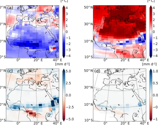
Figure 7. Temperature and precipitation deviations of EHOL from PICTRL in LMDZ-global, the AGCM for (a) winter surface air tempera-tures at 2 m, (b) summer surface air temperatempera-tures at 2 m, (c) June to August precipitation and (d) July to September surface runoff (averaged over the entire simulation).
Figure 8. Deviations (EHOL–PICTRL, averaged over the entire simulation) of surface air temperature at 2 m for winter (a, b) and summer (c, d), respectively. AGCM (LMDZ-global) is displayed in panels (a) and (c) and ARCM (LMDZ-regional) in panels (b) and (d).
JJAS precipitation and JAS surface runoff. The atmospheric model imprints a stronger seasonality due to the increased Early Holocene summer insolation. Warmer summer temper-atures over Europe and north Africa (+6◦C; Fig. 7b) and lower winter temperatures over Africa (−2◦C; Fig. 7a) re-flect this feature. Variations of the precession also trigger an enhancement of the African monsoon (+10 mm d−1over the Ethiopian region; Fig. 7c). The main consequence of this increase in precipitation is an enhanced surface runoff over
the Ethiopian region. This hydrological state is similar to the African Humid Period caused by the enhanced African mon-soon and the resultant increase in surface runoff, as shown in Rossignol-Strick et al. (1982).
Our results are similar to those of previous modelling exercises for the Early Holocene and mid-Holocene (e.g. Adloff et al., 2011; Bosmans et al., 2012; Braconnot et al., 2007; Marzin and Braconnot, 2009). They are also consis-tent with various reconstructions of mid-Holocene
precipi-Figure 9. Winter wind speed in PICTRL for (a) the AGCM and (b) the ARCM.
Figure 10. Same as in Fig. 8 but for precipitation rate (mm d−1).
tation (Harrison et al., 2014). A detailed comparison can be made with the Early Holocene simulation reported in Marzin and Braconnot (2009), who used the same orbital parame-ters and the same atmospheric model as EHOL for their ex-periment. However, their model was coupled to an oceanic model, while an atmospheric model and prescribed SST and SIC as boundary conditions are used in this study. Gener-ally speaking, our results for both surface air temperature and precipitation are very similar to those of Marzin and Bracon-not (2009), attesting to the validity of our approach using a simple atmospheric model constrained by boundary con-ditions. In the ensemble of PMIP simulations, available for the Early Holocene and mid-Holocene, there are some ro-bust outputs for the climate response to orbital forcing but there are also some weaknesses common to most of the mod-els (Braconnot et al., 2007; Kageyama et al., 2013). One of these weaknesses is the underestimation of the spread of the African monsoon towards north Africa. However, the in-creased discharge from the Nile, induced by the enhanced monsoon, is well supported by data (Adamson et al., 1980; Revel et al., 2014; Williams, 2000).
4.3 Mediterranean climate features with dynamical downscaling refinement
Figures 8, 9 and 10 show the results from the regional at-mospheric model (LMDZ-regional) compared to those from LMDZ-global for PICTRL and EHOL over the Mediter-ranean region. In both the global and regional simulations, an increased seasonality is depicted, with warmer summer (+2 to +6◦C) and colder winter, especially over land (−3 to −1◦C; Fig. 8). Downscaling with LMDZ-regional slightly reduces the amplitude of the summer warming and shows a more homogenous signal in winter over land. The general circulation of the surface wind in PICTRL is west to east (Fig. 9b), in line with the dominant winter regime of west-erlies in the region. This important feature is almost missed in the global model (Fig. 9a), which reproduces a lower in-tensity than the regional model. The winter precipitation in EHOL, for ARCM (LMDZ-regional), increases over land in the Balkans and Italy and over the Adriatic, Ionian and Aegean seas (Figure 10b). These changes are also present in the AGCM (LMDZ-global), which furthermore shows an increase in Spain and Portugal (Fig. 10a). It is in summer that the two models show the largest differences. In ARCM (LMDZ-regional), the Mediterranean basin experiences drier conditions, except in Italy and the north of the Balkans. Over the sea, precipitations slightly increase in EHOL (Fig. 10).
However, the AGCM (LMDZ-global) shows drier condi-tions in the northern two-thirds of the Mediterranean domain, with more humid conditions in the southern third (Fig. 10c). Changes in precipitation lead to unavoidable modifications in the runoff and river discharge into the Mediterranean Sea. Although it is not straightforward to compare our “snap-shot” simulations against environmental records (often used to reconstruct a timeline), our results compare well with the available data for this area (see Sect. S3 in the Supplement: comparison of model simulation outputs and reconstructed data for the Mediterranean basin). Numerous proxies pro-vide information on lake levels, paleofires, pollen, isotopic signals recovered from speleothems which together describe the Mediterranean climate in the past. All of these proxies need to be brought together to provide a clear impression of the Mediterranean climate for this period (Magny et al., 2013; Peyron et al., 2011). Magny et al. (2007), based on records from Lago dell’Accesa (Italy), suggested that arid-ification took place around 9200–7700 cal BP. Zanchetta et al. (2007), based on data recovered from speleothems in Italy, concluded that the western Mediterranean basin experienced enhanced rainfall during the S1 (10 000–7000 cal BP). Jalut et al. (2009), using pollen data, suggested that the summers were short and dry, and that there was abundant rainfall in winter (autumn and spring as well), and remarked that these wetter conditions favoured broadleaf tree vegetation. Differ-ent proxies seem to provide contradictory information, and therefore seasonality must be introduced to reconcile them. Peyron et al. (2011) mentioned wet winters and dry summers during the “Holocene optimum”. Magny et al. (2013) support the hypothesis of seasonal contrast based on the analysis of multi-proxies.
Our EHOL simulation successfully depicts this tempera-ture contrast between winter and summer. Precipitation is enhanced in winter. In summer, the Mediterranean region is globally drier, except over northern Italy and the north-ern Balkans. As explained above, there is no precipitation signal over northern Africa, although evidence of paleolakes has been found in Algeria (Callot and Fontugne, 1992; Petit-Maire et al., 1991), Tunisia (Fontes and Gasse, 1991) and Libya (Gaven et al., 1981; Lézine and Casanova, 1991) dur-ing the Early Holocene, indicatdur-ing increased rainfall in this area. In the Supplement, a comparison between simulated continental precipitation outputs and pollen reconstruction data is provided. This comparison shows that the winter pre-cipitation anomalies are consistent in both cases but that there is a distinct difference in summer values due to the more contrasted summer in the EHOL simulation.
4.4 Hydrological changes
Figure 11 shows anomalies (EHOL – PICTRL) of river fresh-water supplies into the Mediterranean basin as simulated by the ARCM (LMDZ-regional). Bars are displayed for each calendar month to show the strong seasonal variation and for
the western and eastern basins separately. Due to their par-ticular role and their specific treatment in our current mod-elling practice, the Nile and the Black Sea are also shown for the eastern basin but not accounted in the sum. The north African rivers are not displayed since they do not show much changes for their catchment area. The Nile shows important seasonal variation, with increase in summer and autumn and decrease in winter and spring. The Albanian rivers (Drini, Mat, Durres, Shkumbin and Vjosa), as well as the Vardar and the Büyük Menderes, produce positive anomalies in EHOL in winter due to enhanced winter land precipitation in this simulation (Fig. 10b and d). The Black Sea net freshwater supply also changes in EHOL with important decreases in January, February, March and July, but increases in April. In EHOL, the supplementary winter freshwater input is less pronounced for the western basin than for the eastern basin (Fig. 11b), but major rivers, such as Rhone and Ebro, do show a strong seasonal cycle. As a whole, the western basin sees an increase of river discharges from March to June.
In terms of areal means for the entire Mediterranean drain-ing basin, the different components of the freshwater bud-get are shown in Table 1 (bottom) for both PICTRL and EHOL, to be compared to the observation-based estima-tion (OBS) and the historical simulaestima-tion (HIST). From PIC-TRL to EHOL, the annual precipitation over the Mediter-ranean Sea itself does not change much, but the annual evaporation amount shows a slight increase (from 1031 to 1094 mm yr−1). However, the most remarkable feature is the increase of river discharges: 98 mm yr−1 in PICTRL to 225 mm yr−1 in EHOL. The total water deficit finally de-creases from 378 to 305 mm yr−1.
4.5 Changes in water properties of the Mediterranean Sea
At the end of our modelling chain, changes in the properties of the Mediterranean seawater produced by NEMOMED8 for PICTRL and EHOL are examined. It is important to men-tion at this stage, that for the correcmen-tion of the river runoff the reference is the pre-industrial state and not the historical sim-ulation (as is the case for SST and SIC). Our aim was to keep river runoff anomalies free of anthropogenic influence. In ad-dition, the fact that the “pre-industrial” Nile river runoff (in other words, before damming) is well known to have influ-enced this choice. Figure 12 shows changes (EHOL minus PICTRL) for sea surface salinities, index of stratification and MLD for the last 30 years of simulation. The EHOL simula-tion reasonably reaches the steady state in terms of IS, ZOF and SSS, as shown in Figs. S6 to S8 of the Supplement. The freshwater inputs from the Nile and the northeastern margin imply a lower salinity in the eastern basin. This decrease in salinity enhances stratification throughout the Mediterranean Sea (with the exception of the western boundary of the east-ern basin, close to the Strait of Sicily) and affects the convec-tion areas by decreasing the MLD, especially in the Gulf of
Figure 11. Monthly anomalies (EHOL–PICTRL, with seasonal variation) of freshwater discharges (m3s−1) for major rivers flowing into the western basin (a) and the eastern basin (b). The sum of all rivers for each basin is also plotted. The Nile and the Black Sea are also shown as rivers of the eastern basin but not accounted into the basin-scale sum.
Figure 12. Deviations between EHOL and PICTRL in (a) sea sur-face salinity, (b) index of stratification and (c) mixed-layer depth, averaged over the last 30 years of simulation.
Lion, in the Adriatic and Ionian seas and in the Aegean. Such a situation is expected and consistent with the basic clima-tology of MLD, shown in Fig. 5. This global stratification in EHOL is followed by a general reduction in the thermohaline circulation compared to PICTRL (ZOF and MOF; Fig. 13).
Numerous studies have documented sapropel event S1 and the state of the Mediterranean Sea that caused it. Emeis et al. (2000) mentioned a decreased SSS during this period in both the eastern and western basins (as did Kallel et al., 1997, in the Tyrrhenian basin). In the “sea surface temperatures” and “sea surface salinity” subsections of Sect. S3 in the Sup-plement, simulated SST and SSS to reconstructions are com-pared. Although simulated SST is in good agreement with the reconstructed data, there is a gap between the simulated SSS and reconstructions. This discrepancy is not surprising. In-deed, there are many explanations for the underestimation in our model of the salinity. One of them is a common weakness in Early Holocene to mid-Holocene simulations, namely, the underestimation of the northward spread of the African mon-soon and therefore the underestimation of the freshwater flow from north Africa. Adloff (2011) already pointed to a short-fall in freshwater input to reconcile the simulated and ob-served SSS during the Early Holocene. Our oceanic simula-tion depicts these behaviours well and is overall similar to previous modelling studies with lower resolution (Adloff et al., 2011; Bosmans et al., 2015; Myers et al., 1998).
Two other issues need to be discussed for the Early Holocene. The first one is sea level, which was 20 m lower than that of the present day (Peltier et al., 2015). For the
Figure 13. ZOF (a) and MOF (b, Gulf of Lion, c, Adriatic/Ionian Sea, d, Aegean Sea) for the EHOL experiment, averaged over the last 30 years of simulation. These overturning stream functions were calculated in the same way as in Fig. 6, providing a strict comparison with the HIST and PICTRL experiments.
sake of simplicity, this difference of sea level is not taken into account in the EHOL simulation. The second issue is the timing of the (re)connection between the Black Sea and the Aegean Sea. This topic is still being debated. Sperling et al. (2003) suggested this reconnection occurred around 8.4 ka, while by the calculations of Soulet et al. (2011) it hap-pened around 9 ka. Other studies found that an overflow from the Black Sea likely occurred before this reconnection due to Fennoscandian ice-sheet melting during the deglaciation (Chepalyga, 2007; Major et al., 2002; Soulet et al., 2011). For the purposes of this work, the Bosphorus is maintained open in EHOL simulation, with the water exchange set at its modern value.
5 Conclusion and perspectives for the modelling platform
This study aimed to develop a modelling platform to simu-late different climatic conditions of the Mediterranean basin. We developed a useful regional climate investigation plat-form with high spatial resolution over the Mediterranean re-gion. This is particularly relevant for the study of impacts on the circulation of the Mediterranean Sea. The model chain has been evaluated for the historical period. We have pre-sented Early Holocene simulations as an example of the
po-tential of this platform to simulate past climate. For the Early Holocene, our model reproduced satisfactorily the global and regional climate features compared to the observed data. Our platform allowed, for the first time, the generation of a high-resolution freshwater budget for this period, with a partic-ular focus on continental precipitation, a key factor for the Mediterranean Sea in the assessment of its impact on circu-lation during the onset of the sapropel event (S1). An impor-tant limitation of our sequential approach is the fact that it does not take account of feedback of ocean changes on atmo-spheric circulation. However, this architecture allows even-tual bias correction, conducted at different levels of the plat-form if needed. One way to overcome this problem of inter-active ocean would be to consider an “asynchronous mode”, namely, to take account of feedback from the ocean compo-nent to the atmosphere at a yearly or decadal frequency.
The modelling sequence, moving from global simulation at low resolution to high-resolution regional ocean mod-elling, avoids the problem of boundary conditions and pro-vides a fully consistent platform that may be used for many paleoclimate studies. We focused here on the Early Holocene period but this architecture could be used to study other pe-riods investigated in model intercomparison projects (MIPs), such as the Last Glacial Maximum or the deposition of older sapropels, from the Pliocene to the Quaternary, as long as the tectonics remain mainly unchanged (PMIP, PlioMIP).
Code and data availability. The current versions of LMDZ and NEMO are available from the project website: https://forge.ipsl. jussieu.fr/igcmg_doc/wiki/Doc/Models/LMDZ (last access: May 2020) and http://forge.ipsl.jussieu.fr/nemo/wiki/Users (last access: May 2020) under the terms of the CeCill license for both LMDZ and NEMO. The exact version of the model used to produce the results used in this paper is archived on Zenodo (Vadsaria et al., 2019), as are input data and scripts to run the model and produce the plots for all the simulations presented in this paper.
Supplement. The supplement related to this article is available on-line at: https://doi.org/10.5194/gmd-13-2337-2020-supplement.
Author contributions. This study was co-designed and approved by all co-authors. The simulation protocol was constructed by TV and LL from a modelling architecture provided by LL. TV con-ducted the numerical simulations and drafted the first version of the manuscript. All co-authors are largely involved in the writing and revision of the manuscript.
Competing interests. The authors declare that they have no conflict of interest.
Acknowledgements. We thank Mary Minnock for her professional English revision. This work was granted access to the HPC re-sources of TGCC under the allocations 2017-A0010102212, 2018-A0030102212 and 2018-A004-01-00239 made by GENCI.
Financial support. This research has been supported by the French National program LEFE “HoMoSapIENS”. Tristan Vadsaria, the first author, was supported by JSPS KAKENHI grant 17H06104.
Review statement. This paper was edited by Lauren Gregoire and reviewed by two anonymous referees.
References
Adamson, D. A., Gasse, F., Street, F. A., and Williams, M. A. J.: Late Quaternary history of the Nile, Nature, 288, 50–55, https://doi.org/10.1038/288050a0, 1980.
Adler, R., Sapiano, M., Huffman, G., Wang, J.-J., Gu, G., Bolvin, D., Chiu, L., Schneider, U., Becker, A., Nelkin, E., Xie, P., Fer-raro, R., and Shin, D.-B.: The Global Precipitation Climatol-ogy Project (GPCP) Monthly Analysis (New Version 2.3) and a Review of 2017 Global Precipitation, Atmosphere, 9, 138, https://doi.org/10.3390/atmos9040138, 2018.
Adloff, F., Mikolajewicz, U., Kuˇcera, M., Grimm, R., Maier-Reimer, E., Schmiedl, G., and Emeis, K.-C.: Corrigendum to “Upper ocean climate of the Eastern Mediterranean Sea during the Holocene Insolation Maximum – a model study” published
in Clim. Past, 7, 1103–1122, 2011, Clim. Past, 7, 1149–1168, https://doi.org/10.5194/cp-7-1149-2011, 2011.
Adloff, F., Somot, S., Sevault, F., Jordà, G., Aznar, R., Déqué, M., Herrmann, M., Marcos, M., Dubois, C., Padorno, E., Alvarez-Fanjul, E., and Gomis, D.: Mediterranean Sea response to cli-mate change in an ensemble of twenty first century scenarios, Clim. Dynam., 45, 2775–2802, https://doi.org/10.1007/s00382-015-2507-3, 2015.
Artale, V.: Role of surface fluxes in ocean general circula-tion models using satellite sea surface temperature: Validacircula-tion of and sensitivity to the forcing frequency of the Mediter-ranean thermohaline circulation, J. Geophys. Res., 107, 3120, https://doi.org/10.1029/2000JC000452, 2002.
Artale, V., Calmanti, S., Carillo, A., Dell’Aquila, A., Herrmann, M., Pisacane, G., Ruti, P. M., Sannino, G., Struglia, M. V., Giorgi, F., Bi, X., Pal, J. S., and Rauscher, S.: An atmosphere–ocean regional climate model for the Mediterranean area: assessment of a present climate simulation, Clim. Dynam., 35, 721–740, https://doi.org/10.1007/s00382-009-0691-8, 2010.
Barnier, B., Siefridt, L., and Marchesiello, P.: Thermal forcing for a global ocean circulation model using a three-year cli-matology of ECMWF analyses, J. Mar. Syst., 6, 363–380, https://doi.org/10.1016/0924-7963(94)00034-9, 1995.
Béranger, K., Drillet, Y., Houssais, M.-N., Testor, P., Bourdallé-Badie, R., Alhammoud, B., Bozec, A., Mortier, L., Bouruet-Aubertot, P., and Crépon, M.: Impact of the spatial distri-bution of the atmospheric forcing on water mass formation in the Mediterranean Sea, J. Geophys. Res., 115, C12041, https://doi.org/10.1029/2009JC005648, 2010.
Beuvier, J., Sevault, F., Herrmann, M., Kontoyiannis, H., Ludwig, W., Rixen, M., Stanev, E., Béranger, K., and Somot, S.: Modeling the Mediterranean Sea interannual variability during 1961–2000: Focus on the Eastern Mediterranean Transient, J. Geophys. Res., 115, C08017, https://doi.org/10.1029/2009JC005950, 2010. Bosmans, J. H. C., Drijfhout, S. S., Tuenter, E., Lourens, L. J.,
Hilgen, F. J., and Weber, S. L.: Monsoonal response to mid-holocene orbital forcing in a high resolution GCM, Clim. Past, 8, 723–740, https://doi.org/10.5194/cp-8-723-2012, 2012. Bosmans, J. H. C., Drijfhout, S. S., Tuenter, E., Hilgen,
F. J., Lourens, L. J., and Rohling, E. J.: Preces-sion and obliquity forcing of the freshwater budget over the Mediterranean, Quat. Sci. Rev., 123, 16–30, https://doi.org/10.1016/j.quascirev.2015.06.008, 2015.
Braconnot, P., Otto-Bliesner, B., Harrison, S., Joussaume, S., Pe-terchmitt, J.-Y., Abe-Ouchi, A., Crucifix, M., Driesschaert, E., Fichefet, Th., Hewitt, C. D., Kageyama, M., Kitoh, A., Laîné, A., Loutre, M.-F., Marti, O., Merkel, U., Ramstein, G., Valdes, P., Weber, S. L., Yu, Y., and Zhao, Y.: Results of PMIP2 coupled simulations of the Mid-Holocene and Last Glacial Maximum – Part 1: experiments and large-scale features, Clim. Past, 3, 261– 277, https://doi.org/10.5194/cp-3-261-2007, 2007.
Callot, Y. and Fontugne, M.: Les étagements de nappes dans les paléolacs holocènes du nord-est du Grand Erg Occidental (Al-gérie), Comptes-Rendus de l’Académie des Sciences, Paris, 315, II, 471–477, 1992.
Chen, J., Brissette, F. P., and Leconte, R.: Uncertainty of downscaling method in quantifying the impact of cli-mate change on hydrology, J. Hydrol., 401, 190–202, https://doi.org/10.1016/j.jhydrol.2011.02.020, 2011.
Chepalyga, A. L.: The late glacial great flood in the Ponto-Caspian basin, in The Black Sea Flood Question: Changes in Coastline, Climate, and Human Settlement, Springer Netherlands, 119–148, 2007.
De Lange, G. J., Thomson, J., Reitz, A., Slomp, C. P., Speranza Principato, M., Erba, E., and Corselli, C.: Syn-chronous basin-wide formation and redox-controlled preserva-tion of a Mediterranean sapropel, Nat. Geosci., 1, 606–610, https://doi.org/10.1038/ngeo283, 2008.
De Zolt, S., Lionello, P., and Malguzzi, P.: Implementation of an AORCM in the Mediterranean Sea, Geophys. Res. Abs. 5, EAE03-A-08425 EGS-AGU–EUG Joint Assembly, Nice, France, 6–11 April 2003.
Dee, D. P., Uppala, S. M., Simmons, A. J., Berrisford, P., Poli, P., Kobayashi, S., Andrae, U., Balmaseda, M. A., Balsamo, G., Bauer, P., Bechtold, P., Beljaars, A. C. M., van de Berg, I., Biblot, J., Bormann, N., Delsol, C., Dragani, R., Fuentes, M., Greer, A. J., Haimberger, L., Healy, S. B., Hersbach, H., Holm, E. V., Isak-sen, L., Kallberg, P., Kohler, M., Matricardi, M., McNally, A. P., Mong-Sanz, B. M., Morcette, J.-J., Park, B.-K., Peubey, C., de Rosnay, P., Tavolato, C., Thepaut, J. N., and Vitart, F.: The ERA-Interim reanalysis: Configuration and performance of the data assimilation system, Q. J. Roy. Meteorol. Soc., 137, 553–597, https://doi.org/10.1002/qj.828, 2011.
Dell’Aquila, A., Calmanti, S., Ruti, P., Struglia, M., Pisacane, G., Carillo, A., and Sannino, G.: Effects of seasonal cycle fluctua-tions in an A1B scenario over the Euro-Mediterranean region, Clim. Res., 52, 135–157, https://doi.org/10.3354/cr01037, 2012. Drobinski, P., Anav, A., Lebeaupin Brossier, C., Samson, G., Stéfanon, M., Bastin, S., Baklouti, M., Béranger, K., Beu-vier, J., Bourdallé-Badie, R., Coquart, L., D’Andrea, F., de Noblet-Ducoudré, N., Diaz, F., Dutay, J.-C., Ethe, C., Fou-jols, M.-A., Khvorostyanov, D., Madec, G., Mancip, M., Mas-son, S., Menut, L., Palmieri, J., Polcher, J., Turquety, S., Val-cke, S., and Viovy, N.: Model of the Regional Coupled Earth system (MORCE): Application to process and climate stud-ies in vulnerable regions, Environ. Model. Softw., 35, 1–18, https://doi.org/10.1016/j.envsoft.2012.01.017, 2012.
Dufresne, J.-L., Foujols, M.-A., Denvil, S., Caubel, A., Marti, O., Aumont, O., Balkanski, Y., Bekki, S., Bellenger, H., Benshila, R., Bony, S., Bopp, L., Braconnot, P., Brockmann, P., Cadule, P., Cheruy, F., Codron, F., Cozic, A., Cugnet, D., de Noblet, N., Duvel, J.-P., Ethé, C., Fairhead, L., Fichefet, T., Flavoni, S., Friedlingstein, P., Grandpeix, J.-Y., Guez, L., Guilyardi, E., Hauglustaine, D., Hourdin, F., Idelkadi, A., Ghattas, J., Jous-saume, S., Kageyama, M., Krinner, G., Labetoulle, S., Lahel-lec, A., Lefebvre, M.-P., Lefevre, F., Levy, C., Li, Z. X., Lloyd, J., Lott, F., Madec, G., Mancip, M., Marchand, M., Masson, S., Meurdesoif, Y., Mignot, J., Musat, I., Parouty, S., Polcher, J., Rio, C., Schulz, M., Swingedouw, D., Szopa, S., Talandier, C., Terray, P., Viovy, N., and Vuichard, N.: Climate change projections us-ing the IPSL-CM5 Earth System Model: from CMIP3 to CMIP5, Clim. Dynam., 40, 2123–2165, https://doi.org/10.1007/s00382-012-1636-1, 2013.
Emeis, K.-C., Struck, U., Schulz, H.-M., Rosenberg, R., Bernasconi, S., Erlenkeuser, H., Sakamoto, T., and Martinez-Ruiz, F.: Temperature and salinity variations of Mediter-ranean Sea surface waters over the last 16,000 years from records of planktonic stable oxygen isotopes and alkenone
unsaturation ratios, Palaeogeogr. Palaeocl., 158, 259–280, https://doi.org/10.1016/S0031-0182(00)00053-5, 2000. Fontes, J. C. and Gasse, F.: PALHYDAF (Palaeohydrology in
Africa) program: objectives, methods, major results, Palaeo-geogr. Palaeocl., 84, 191–215, https://doi.org/10.1016/0031-0182(91)90044-R, 1991.
Gaven, C., Hillaire-Marcel, C., and Petit-Maire, N.: A Pleistocene lacustrine episode in southeastern Libya, Nature, 290, 131–133, https://doi.org/10.1038/290131a0, 1981.
Giorgi, F.: Climate change hot-spots, Geophys. Res. Lett., 33, L08707, https://doi.org/10.1029/2006GL025734, 2006. Goubanova, K. and Li, L.: Extremes in temperature and
precipi-tation around the Mediterranean basin in an ensemble of future climate scenario simulations, Glob. Planet. Change, 57, 27–42, https://doi.org/10.1016/j.gloplacha.2006.11.012, 2007.
Harrison, S. P., Bartlein, P. J., Brewer, S., Prentice, I. C., Boyd, M., Hessler, I., Holmgren, K., Izumi, K., and Willis, K.: Climate model benchmarking with glacial and mid-Holocene climates, Clim. Dynam., 43, 671–688, https://doi.org/10.1007/s00382-013-1922-6, 2014.
Hernández-Díaz, L., Laprise, R., Nikiéma, O., and Winger, K.: 3-Step dynamical downscaling with empirical correction of sea-surface conditions: application to a CORDEX Africa simulation, Clim. Dynam., 48, 2215–2233, https://doi.org/10.1007/s00382-016-3201-9, 2017.
Herrmann, M., Sevault, F., Beuvier, J., and Somot, S.: What induced the exceptional 2005 convection event in the northwestern Mediterranean basin? Answers from a modeling study, J. Geophys. Res., 115, C12051, https://doi.org/10.1029/2010JC006162, 2010.
Houpert, L., Testor, P., Durrieu de Madron, X., Somot, S., D’Ortenzio, F., Estournel, C., and Lavigne, H.: Seasonal cy-cle of the mixed layer, the seasonal thermocline and the upper-ocean heat storage rate in the Mediterranean Sea de-rived from observations, Prog. Oceanogr., 132, 333–352, https://doi.org/10.1016/j.pocean.2014.11.004, 2015.
Hourdin, F., Musat, I., Bony, S., Braconnot, P., Codron, F., Dufresne, J.-L., Fairhead, L., Filiberti, M.-A., Friedlingstein, P., Grandpeix, J.-Y., Krinner, G., LeVan, P., Li, Z.-X., and Lott, F.: The LMDZ4 general circulation model: climate per-formance and sensitivity to parametrized physics with em-phasis on tropical convection, Clim. Dynam., 27, 787–813, https://doi.org/10.1007/s00382-006-0158-0, 2006.
Jalut, G., Dedoubat, J. J., Fontugne, M., and Otto, T.: Holocene circum-Mediterranean vegetation changes: Cli-mate forcing and human impact, Quat. Int., 200, 4–18, https://doi.org/10.1016/j.quaint.2008.03.012, 2009.
Jost, A., Lunt, D., Kageyama, M., Abe-Ouchi, A., Peyron, O., Valdes, P. J., and Ramstein, G.: High-resolution simulations of the last glacial maximum climate over Europe: a solution to discrepancies with continental palaeoclimatic reconstructions?, Clim. Dynam., 24, 577–590, https://doi.org/10.1007/s00382-005-0009-4, 2005.
Kageyama, M., Braconnot, P., Bopp, L., Caubel, A., Foujols, M.-A., Guilyardi, E., Khodri, M., Lloyd, J., Lombard, F., Mariotti, V., Marti, O., Roy, T., and Woillez, M.-N.: Mid-Holocene and Last Glacial Maximum climate simulations with the IPSL model – part I: comparing IPSL_CM5A to IPSL_CM4, Clim.
Dy-nam., 40, 2447–2468, https://doi.org/10.1007/s00382-012-1488-8, 2013.
Kallel, N., Paterne, M., Labeyrie, L., Duplessy, J.-C., and Arnold, M.: Temperature and salinity records of the Tyrrhenian Sea dur-ing the last 18,000 years, Palaeogeogr. Palaeocl., 135, 97–108, https://doi.org/10.1016/S0031-0182(97)00021-7, 1997. Kourafalou, V. H. and Barbopoulos, K.: High resolution simulations
on the North Aegean Sea seasonal circulation, Ann. Geophys., 21, 251–265, https://doi.org/10.5194/angeo-21-251-2003, 2003. Krinner, G., Viovy, N., de Noblet-Ducoudré, N., Ogée, J., Polcher, J., Friedlingstein, P., Ciais, P., Sitch, S., and Prentice, I. C.: A dynamic global vegetation model for studies of the coupled atmosphere-biosphere system, Global Biogeochem. Cy., 19, 1– 33, https://doi.org/10.1029/2003GB002199, 2005.
Krinner, G., Largeron, C., Ménégoz, M., Agosta, C., and Brutel-Vuilmet, C.: Oceanic Forcing of Antarctic Climate Change: A Study Using a Stretched-Grid Atmospheric General Circulation Model, J. Clim., 27, 5786–5800, https://doi.org/10.1175/JCLI-D-13-00367.1, 2014.
Krinner, G., Beaumet, J., Favier, V., Déqué, M., and Brutel-Vuilmet, C.: Empirical Run-Time Bias Correction for Antarctic Regional Climate Projections With a Stretched-Grid AGCM, J. Adv. Model. Earth Sy., 11, 64–82, https://doi.org/10.1029/2018MS001438, 2019.
Lacombe, H. and Tchernia, P.: Caractères hydrologiques et circu-lation des eaux en Méditerranée, in: The Mediterranean Sea: A natural sedimentation laboratory, edited by: Stanley, D., Dowden, Hutchinson & Ross, Stroudsburg, 25–36, 1972.
Lebeaupin Brossier, C., Béranger, K., Deltel, C., and Drobin-ski, P.: The Mediterranean response to different space– time resolution atmospheric forcings using perpetual mode sensitivity simulations, Ocean Model., 36, 1–25, https://doi.org/10.1016/j.ocemod.2010.10.008, 2011.
Lézine, A.-M. and Casanova, J.: Correlated oceanic and continental records demonstrate past climate and hydrology of North Africa (0–140 ka), Geology, 19, 307–310, https://doi.org/10.1130/0091-7613(1991)019<0307:COACRD>2.3.CO;2, 1991.
Li, L., Bozec, A., Somot, S., Bouruet-Aubertot, P., and Crepon, M.: Regional atmospheric, marine processes and climate modelling, in Mediterranean climate variability and predictability, edited by: Lionello, P., Malanotte-Rizzoli, P., and Boscolo, R., Elsevier, 2006.
Li, L., Casado, A., Congedi, L., Dell’Aquila, A., Dubois, C., Elizalde, A., L’Hévéder, B., Lionello, P., Sevault, F., Somot, S., Ruti, P., and Zampieri, M.: Modeling of the mediterranean cli-mate system, in The Clicli-mate of the Mediterranean Region, Else-vier Inc., 419–448, 2012.
Li, Z.-X.: Ensemble Atmospheric GCM Simulation of Climate Interannual Variability from 1979 to 1994, J. Clim., 12, 986–1001, https://doi.org/10.1175/1520-0442(1999)012<0986:EAGSOC>2.0.CO;2, 1999.
Locarnini, R. A., Mishonov, A. V., Antonov, J. I., Boyer, T. P., Gar-cia, H. E., Baranova, O. K., Zweng, M. M., Paver, C. R., Reagan, J. R., Johnson, D. R., Hamilton, M., and Seidov, D.: World Ocean Atlas 2013, Vol. 1: Temperature, edited by: Levitus, S., NOAA Atlas NESDIS 73, 40 pp., 2013.
Ludwig, P., Shao, Y., Kehl, M., and Weniger, G.-C.: The Last Glacial Maximum and Heinrich event I on the Iberian Penin-sula: A regional climate modelling study for understanding
hu-man settlement patterns, Glob. Planet. Change, 170, 34–47, https://doi.org/10.1016/j.gloplacha.2018.08.006, 2018.
Ludwig, W., Dumont, E., Meybeck, M., and Heussner, S.: River discharges of water and nutrients to the Mediterranean and Black Sea: Major drivers for ecosystem changes dur-ing past and future decades?, Prog. Oceanogr., 80, 199–217, https://doi.org/10.1016/j.pocean.2009.02.001, 2009.
Macias, D. M., Garcia-Gorriz, E., and Stips, A.: Productivity changes in the Mediterranean Sea for the twenty-first century in response to changes in the regional atmospheric forcing, Front. Mar. Sci., 2, 79, https://doi.org/10.3389/fmars.2015.00079, 2015.
Madec, G.: NEMO ocean engine-version 3.0-Laboratoire d’Océanographie et du Climat: Expérimentation et Approches Numériques, 2008.
Magny, M., de Beaulieu, J.-L., Drescher-Schneider, R., Vannière, B., Walter-Simonnet, A.-V., Miras, Y., Millet, L., Bossuet, G., Peyron, O., Brugiapaglia, E., and Leroux, A.: Holocene climate changes in the central Mediterranean as recorded by lake-level fluctuations at Lake Accesa (Tuscany, Italy), Quat. Sci. Rev., 26, 1736–1758, https://doi.org/10.1016/j.quascirev.2007.04.014, 2007.
Magny, M., Combourieu-Nebout, N., de Beaulieu, J. L., Bout-Roumazeilles, V., Colombaroli, D., Desprat, S., Francke, A., Joannin, S., Ortu, E., Peyron, O., Revel, M., Sadori, L., Siani, G., Sicre, M. A., Samartin, S., Simonneau, A., Tinner, W., Vannière, B., Wagner, B., Zanchetta, G., Anselmetti, F., Brugiapaglia, E., Chapron, E., Debret, M., Desmet, M., Didier, J., Essallami, L., Galop, D., Gilli, A., Haas, J. N., Kallel, N., Millet, L., Stock, A., Turon, J. L., and Wirth, S.: North–south palaeohydrological contrasts in the central Mediterranean during the Holocene: ten-tative synthesis and working hypotheses, Clim. Past, 9, 2043– 2071, https://doi.org/10.5194/cp-9-2043-2013, 2013.
Major, C., Ryan, W., Lericolais, G., and Hajdas, I.: Constraints on Black Sea outflow to the Sea of Marmara during the last glacial–interglacial transition, Mar. Geol., 190, 19–34, https://doi.org/10.1016/S0025-3227(02)00340-7, 2002. Marzin, C. and Braconnot, P.: Variations of Indian and African
monsoons induced by insolation changes at 6 and 9.5 kyr BP, Clim. Dynam., 33, 215–231, https://doi.org/10.1007/s00382-009-0538-3, 2009.
Mikolajewicz, U.: Modeling Mediterranean Ocean climate of the Last Glacial Maximum, Clim. Past, 7, 161–180, https://doi.org/10.5194/cp-7-161-2011, 2011.
Millot, C. and Taupier-Letage, I.: Circulation in the Mediterranean Sea, 29–66, 2005.
Myers, P. G., Haines, K., and Rohling, E. J.: Modeling the paleocirculation of the Mediterranean: The Last Glacial Maximum and the Holocene with emphasis on the for-mation of sapropel S1, Paleoceanography, 13, 586–606, https://doi.org/10.1029/98PA02736, 1998.
Peltier, W. R., Argus, D. F., and Drummond, R.: Space geodesy constrains ice age terminal deglaciation: The global ICE-6G_C (VM5a) model, J. Geophys. Res.-Sol. Ea., 120, 450–487, https://doi.org/10.1002/2014JB011176, 2015.
Petit-Maire, N., Fontugne, M., and Rouland, C.: Atmospheric methane ratio and environmental change in the Sahara an Sahel during the last 130 kyrs, Palaeogeogr. Palaeocl., 86, 197–206, https://doi.org/10.1016/0031-0182(91)90009-G, 1991.