HAL Id: hal-03229033
https://hal.archives-ouvertes.fr/hal-03229033
Submitted on 18 May 2021
HAL is a multi-disciplinary open access
archive for the deposit and dissemination of
sci-entific research documents, whether they are
pub-lished or not. The documents may come from
teaching and research institutions in France or
abroad, or from public or private research centers.
L’archive ouverte pluridisciplinaire HAL, est
destinée au dépôt et à la diffusion de documents
scientifiques de niveau recherche, publiés ou non,
émanant des établissements d’enseignement et de
recherche français ou étrangers, des laboratoires
publics ou privés.
To cite this version:
Oscar Rojas, Marjolaine Chiriaco, Sophie Bastin, Justine Ringard. Estimation of the terms acting
on local surface one-hour temperature variations in Paris region: the specific contribution of clouds.
Atmospheric Chemistry and Physics Discussions, European Geosciences Union, 2021, pp.(Under
Re-view). �10.5194/acp-2021-370�. �hal-03229033�
Estimation of the terms acting on local surface one-hour temperature
variations in Paris region: the specific contribution of clouds
Oscar Rojas
1, Marjolaine Chiriaco
1, Sophie Bastin
1, Justine Ringard
11 LATMOS/IPSL, UVSQ, Université Paris-Saclay, Sorbonne Université, CNRS, 78280, Guyancourt, France
5
Correspondence to: Oscar Rojas ([email protected])
Abstract. Local temperature variations at the surface are mainly dominated by small-scale processes coupled through the surface energy budget terms, which depend mostly on radiation availability and thus cloud processes. A method to determine each of these terms based almost exclusively on observations is presented in this paper, with the main objective to estimate their importance in hourly surface temperature variations at the SIRTA observatory, near Paris. Almost all terms are estimated 10
from the multi-year dataset SIRTA-ReOBS, following a few parametrizations. The four main terms acting on temperature variations are radiative forcing (separated into clear-sky and cloud radiation), atmospheric heat exchange, ground heat exchange, and advection. Compared to direct measurements of hourly temperature variations, it is shown that the sum of the four terms gives a good estimate of the hourly temperature variations, allowing a better assessment of the contribution of each term to the variation, with an accurate diurnal and annual cycles representation, especially for the radiative terms. A random 15
forest analysis shows that whatever the season, clouds are the main modulator of the clear sky radiation for 1-hour temperature variations during the day, and mainly drive these 1-hour temperature variations during the night. Then, the specific role of clouds is analyzed exclusively in cloudy conditions considering the behavior of some classical meteorological variables along with lidar profiles. Cloud radiative effect in shortwave and longwave and lidar profiles show a consistent seasonality during the daytime, with a dominance of mid- and high-level clouds detected at the SIRTA observatory, which also affects surface 20
temperatures and upward sensible heat flux. During the nighttime, despite cloudy conditions and having a strong cloud longwave radiative effect, temperatures are the lowest and are therefore mostly controlled by larger-scale processes at this time.
1 Introduction
Regional climate variability is to the first order driven by large-scale atmospheric conditions. In Western Europe, the North 25
Atlantic Oscillation (NAO; Trigo et al., 2002), which is associated with the locations and intensities of the centers of the Iceland low and the Açores high, controls the air mass advection over western Europe and explains a large part of variability. Temperature and pressure conditions are then modulated by the complex terrain (Mediterranean sea, topography, surface heterogeneities): extreme events and temperature anomalies are generally not exclusively explained by the presence of these
large-scale air mass circulations (Vautard and Yiou, 2009). It is, therefore, necessary to consider small-scale processes such 30
as surface-atmosphere interactions and cloud feedbacks to better explain surface temperature variations (e.g. Chiriaco et al., 2014).
Temperature variations at the surface are related to the Surface Energy Balance (SEB) following surface-atmosphere interactions and solar radiation (Wang and Dickinson, 2013) that are separated into different components: latent and sensible heat fluxes (Flat and Fsens, respectively), ground heat flux, air advection, and atmosphere radiation. Studies have been made
35
to parametrize these terms when direct measurements are not available (Miller et al. 2017; Arnold et al. 1996) but their exact contribution is uncertain. Depending on the time-scale considered, the importance of each SEB term on temperature variations will change (Bastin et al. 2018; Ionita et al. 2015).
The first objective of the current paper is to quantify the specific local contribution of the primary SEB terms acting on short-term (i.e. hourly) temperature variations in a Western European location and to deshort-termine their importance and the conditions 40
when a certain term predominates over the others, based on a simple linear model. The current study is inspired by Bennartz et al. (2013) who implemented a temperature variation model to study the influence of low-level liquid clouds over the Arctic on the ice surface melt period in July 2012, by estimating all of these SEB terms for a case study. Here, the same approach is used for a different location (mid-latitude) and on a long-time period to get robust statistics. To do so, the study is based on direct measurements from the SIRTA-ReOBS dataset (Chiriaco et al., 2018), which includes many variables collected since 45
2002 at SIRTA (Site Instrumental de Recherche en Télédetection Active; Haeffelin et al. 2005), an observatory located in a semi-urban area in the Southwest of Paris, France. This dataset is well suited to the current study objective because: (i) it allows the use of a multi-variable synergistic compilation to study and compare different characteristics of the atmosphere or the surface (e.g. Bastin et al. 2018; Dione et al. 2017; Cheruy et al. 2013, Chiriaco et al., 2014), (ii) it is located in Western Europe and allows access to the hourly time scale, i.e. the scales of the local processes of the current study. The SIRTA-ReOBS 50
dataset, along with some variables retrieved from ERA5 Reanalysis, enables the development of a model to estimate all the terms involved in the surface temperature variations using predominantly real observations. The weight of each term of the SEB on hourly temperature variations is analyzed using a powerful random forest analysis whose maximal advantage is its capacity to handle up to thousands of input variables and identify the most significant ones.
The main result of this first objective is the fact that clouds are the main modulator on hourly temperature variations for most 55
of the hours of the day and all the seasons. Hence the second objective of the current study is to understand the specific role of clouds and their associated characteristics on hourly temperature variations. Indeed, the influence of clouds on the temperature at the surface can vary depending on their physical properties and the altitude where they are formed (Hartmann et al., 1992; Chen et al., 2000). In general, low-level clouds tend to cool the surface, whereas high-level clouds, such as cirrus clouds, tend to warm it by absorbing a significant amount of Earth’s outgoing radiation. The average contribution of clouds is 60
to decrease the surface temperature, combined with the damping effects of soil moisture, from a global point of view, by reflecting the solar radiation to space. But their damping effects vary depending on the season and the state of the atmosphere. For instance, the reduction in surface temperature is the highest in fall in northern mid-latitudes for specific cases when
precipitation is not significant (Dai et al. 1999). The local contribution of clouds to temperature variations is thus an important topic to assess how this intake affects local climate variability and extreme local events. Several studies were made primarily 65
focusing on the large scale effects of clouds on the radiative energy balance on a global scale, either at the top of the atmosphere (Arkin and Meisner, 1987; Raschke et al., 2005; Dewitte and Clerbaux, 2017; Willson et al., 1981; Allan et al., 2014; Cherviakov, 2016) or at the surface (Wild et al., 2015; Hakuba et al., 2013; Wild, 2017) or both at the same time (Hartmann, 1993; Kato et al., 2012; Li and Leighton, 1993), but a lack of studies investigating their impact on a smaller scale is noted due to limited reliable ground-based measurement availability. In this study, to understand how clouds influence the one-hour 70
temperature variations, cases with a predominance of cloud effect on temperature variations are analyzed specifically with lidar profiles to understand the role of the vertical distribution of clouds and their radiative effect on the state of the atmosphere. To answer these two objectives, the current paper is organized as follows: the dataset is presented in Section 2. Section 3 (and Appendix A) consists of describing how the different terms acting on hourly temperature variations are estimated and evaluating how well the model fits the hourly observations based on statistics. Section 4 presents an assessment to determine 75
which term dominates at different times by performing a random forest analysis firstly for day and night cases, and then separated in a diurnal cycle perspective, along with a mean monthly-hourly and annual cycles analysis of the contribution of each term. Section 5 focuses on a discussion to study the specific role of clouds and the atmospheric conditions under which they develop by assessing only the cloudy cases, which gives an overview of the type of clouds and surface conditions damping or enhancing surface temperature for both day and nighttime. Section 6 draws conclusions and provides perspectives opened 80
by this work.
2 Data
2.1 Data used for the temperature variations estimation model
This study is mainly based on the SIRTA-ReOBS dataset analysis. The SIRTA observatory (Haeffelin et al. 2005) is located 85
in a semi-urban area 20-km Southwest of Paris (48.71° N, 2.2° E) and has collected long-term meteorological variables since 2002. The ReOBS project aims to synthesize all observations available at a single observatory at an hourly time scale with an exhaustive data-quality control, calibration, and rigorous treatment, into a single NetCDF file. The SIRTA-ReOBS dataset (Chiriaco et al. 2018, https://doi.org/10.5194/essd-10-919-2018) contains more than 60 variables.
All the necessary hourly variables requested by the current study are available for the period going from January 2009 to 90
February 2014 and are listed in Table 1, allowing the performance of a multi-year analysis. Some variables that were retrieved from measurements at the SIRTA observatory sometimes present gaps due to instrumental issues (Chiriaco et al. 2018; Pal and Haeffelin 2015). In particular Flat and Fsens variables are limited (with only 5% and 73% availability, respectively): Sect.
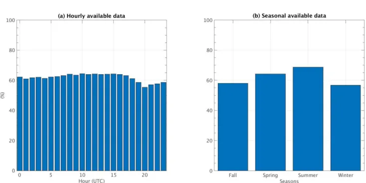
Figure 1 shows the complete dataset availability in the SIRTA-ReOBS dataset for the five-year study period. The availability 95
of data is quasi-homogeneous around 60% for all hours (Figure 1a). Gaps are most of the time due to the absence of the Mixing Layer Depth (MLD) variable for some complete days, extended sometimes for more than two months (not shown), restricting 71% of MLD data availability. Other gaps are caused by the absence of radiative variables (9% of missing data, see Table 1). Summer is the season with the best data coverage (70%) and winter with the least data coverage (56% - Figure 1b), whose absences are due precisely to gaps in the MLD variable.
100
To complete this dataset, ERA5 hourly Reanalysis (spatial resolution of 31 km and 137 levels up to 1 hPa; ERA5: Fifth generation of ECMWF atmospheric reanalyses of the global climate, 2020) is used to estimate the horizontal wind at 10 m (useful to estimate the advection – see Section 3) and the temperature at the mixing layer depth (𝑇𝑀𝐿𝐷 - see Section 3.1 and
Appendix).
2.2 Variables used for the cloud contribution analysis 105
In order to get vertical information about clouds (see Section 5), SIRTA-ReOBS lidar profiles are also used, based on hourly lidar Scattering Ratio altitude-intensity histograms, calculated as follows:
𝑆𝑅(𝑧) = 𝐴𝑇𝐵(𝑧)
𝐴𝑇𝐵(𝑧)𝑚𝑜𝑙 (1) Where ATB(z) is defined as the total attenuated backscatter lidar signal and ATB(z)mol is the signal in clear-sky conditions.
These altitude-intensity histograms are used to estimate the mean cloud fraction percentage at a given altitude level z. The 110
intensity axis which contains SR(z) thresholds as well as the three vertical atmospheric layers (i.e. low, middle and high-level layers) for cloud detection and characterization are defined in(Chepfer et al. (2010). The value of SR(z) = -999 corresponds to non-normalized profiles, the value -777 represents the profiles that cannot be normalized due to the presence of a very low opaque cloud and the value of -666 is set as invalid data. Then, bins located in the range 0.01<SR(z)<1 are for clear-sky conditions, 1.2<SR(z)<5 is defined as unclassified data, and for cloud detection, a threshold of SR(z)>5 is set. Details are given 115
in Chiriaco et al. (2018). Even though the instrument does not operate uninterrupted (it does not operate when it is raining, when it’s nighttime, and on the weekends), it is very powerful to get information on the vertical structure of the atmosphere and so understand the category of clouds acting on the temperature variations.
3 Estimation of the terms acting on surface temperature variations
The exchange of energy between the surface and the overlying atmosphere involves four terms: radiation, heat exchange with 120
ground, heat exchange with the free atmosphere, and advection. In this section, a model which estimates these four terms is presented, based on several meteorological observations retrieved from the SIRTA-ReOBS dataset. Each term involved in this model is described (further descriptions are presented in Appendix), and then a statistical evaluation is performed to assess how well the model follows the real observations of temperature variations. Finally, the mean monthly-hourly and annual
cycles of the averaged contribution of each term and the same for temperature 1-hour variations (𝜕𝑇2𝑚
𝜕𝑡 𝑜𝑏𝑠) are presented (split
125
into day and night).
3.1 Model description
The temperature variation at the surface is estimated from the sum of four terms:
𝜕𝑇2𝑚
𝜕𝑡 = 𝑅 + 𝐻𝐺 + 𝐻𝐴 + 𝐴𝑑𝑣
(2)
Where R is the net radiative flux at the surface, HG is the ground heat exchange, HA is the atmospheric heat exchange, and 130
Adv is the air advection. These four terms control the changes in temperature over the surface, but depending on the temporal scale, one will dominate over the others (Ionita et al., 2012). Following the Appendix and partly based on(Bennartz et al. (2013),)these four terms are expressed as:
𝑅 = 𝛼+1 𝜌𝑐𝑝𝑀𝐿𝐷∆𝐹𝑁𝐸𝑇 (3) 𝐻𝐺 =𝑇𝑠−𝑇2𝑚 𝜏𝑠 (4) 135 𝐻𝐴 =𝑇𝑀𝐿𝐷−𝑇2𝑚 𝜏𝑎 (5) 𝐴𝑑𝑣 = (𝑢10 𝜕𝑇2𝑚 𝜕𝑥 + 𝑣10 𝜕𝑇2𝑚 𝜕𝑦 ) (6) Then: 𝜕𝑇2𝑚 𝜕𝑡 = 𝛼+1 𝜌𝑐𝑝𝑀𝐿𝐷∆𝐹𝑁𝐸𝑇+ 𝑇𝑠−𝑇2𝑚 𝜏𝑠 + 𝑇𝑀𝐿𝐷−𝑇2𝑚 𝜏𝑎 − (𝑢10 𝜕𝑇2𝑚 𝜕𝑥 + 𝑣10 𝜕𝑇2𝑚 𝜕𝑦 )
(7)
Where 𝑇2𝑚 is the surface temperature, 𝑡 is the time (in hours), 𝛼 is a coefficient characterizing the form of the temperature
140
vertical profile in the boundary layer, 𝜌 is the average air density of the boundary layer, 𝑐𝑝 is the specific heat of air, MLD is
the mixing layer depth, ∆𝐹𝑁𝐸𝑇 is the net radiative flux at the surface, 𝑇𝑠 is the temperature in the ground at 20 cm depth, 𝑇𝑀𝐿𝐷
is the temperature at the top of the boundary layer (or mixed layer depth), 𝑢10 and 𝑣10 are the zonal and meridional wind
components respectively at 10 m above the ground, and 𝜏𝑠 and 𝜏𝑎 are defined as relaxation timescales for heat exchange
processes in the ground and the atmosphere, respectively. 145
If the model is realistic, then the sum of the four terms in the left side of Eq. (2), denoted as 𝜕𝑇2𝑚
𝜕𝑡 𝑚𝑜𝑑, is as close as possible to
the observed temperature variations denoted as 𝜕𝑇2𝑚
𝜕𝑡 𝑜𝑏𝑠.
The net radiative flux at the surface is calculated as the difference between the radiative longwave (LW) and shortwave (SW) fluxes leaving and arriving at the surface as follows:
∆𝐹𝑁𝐸𝑇= 𝐹𝑆𝑊↓ − 𝐹𝑆𝑊↑ + 𝐹𝐿𝑊↓ − 𝐹𝐿𝑊↑ (8)
150
Where the upward and downward arrows represent the upwelling and downwelling radiation, respectively. It is possible to add and subtract the clear-sky (CS) downwelling radiation fluxes to Eq. (8), to obtain the flux radiative components in CS and cloudy (CL) conditions (i.e. the specific contribution of clouds), as follows:
∆𝐹𝑁𝐸𝑇= 𝐹𝑆𝑊↓ − 𝐹𝑆𝑊↑ + 𝐹𝐿𝑊↓ − 𝐹𝐿𝑊↑ + 𝐹𝑆𝑊,𝐶𝑆↓ − 𝐹𝑆𝑊,𝐶𝑆↓ + 𝐹𝐿𝑊,𝐶𝑆↓ − 𝐹𝐿𝑊,𝐶𝑆↓
∆𝐹𝑁𝐸𝑇= 𝐹𝑆𝑊↓ − 𝐹𝑆𝑊,𝐶𝑆↓ + 𝐹𝐿𝑊↓ − 𝐹𝐿𝑊,𝐶𝑆↓ + 𝐹𝑆𝑊,𝐶𝑆↓ − 𝐹𝑆𝑊↑ + 𝐹𝐿𝑊,𝐶𝑆↓ − 𝐹𝐿𝑊↑ (9)
155
Here, the 𝐹𝐿𝑊↑ flux is the same for clear-sky and cloudy conditions, because it mostly depends on the surface temperature (i.e.
the Stefan-Boltzmann law, 𝐹↑= 𝜎𝑇
2𝑚4 , where 𝜎 is the Stefan-Boltzmann constant), but note that in an annual global mean,
𝐹𝐿𝑊↑ > 𝐹𝐿𝑊,𝐶𝑆↑ (around 0.5 W m-2; Allan 2011) due to the increase in longwave radiation emitted toward the surface by clouds,
160
where a small proportion of this radiation is reflected by the surface. Hence Eq. (2) becomes:
𝜕𝑇2𝑚 𝜕𝑡 = 𝑅𝐶𝐿+ 𝑅𝐶𝑆+ 𝐻𝐺 + 𝐻𝐴 + 𝐴𝑑𝑣 (10) With 𝑅𝐶𝐿 = 𝛼+1 𝜌𝑐𝑝𝑀𝐿𝐷∆𝐹𝑁𝐸𝑇,𝐶𝐿 and 𝑅𝐶𝑆= 𝛼+1 𝜌𝑐𝑝𝑀𝐿𝐷∆𝐹𝑁𝐸𝑇,𝐶𝑆
This formulation specifically allows estimation of the role of clouds (RCL) in temperature variations, compared to the other
165
terms. Details on how each term is estimated along with the assumptions that have been made are stated in the Appendix. As shown by Eq. (3) to Eq. (6) and in the Appendix, temperature variations are estimated from variables described in Section 2, i.e. predominantly based on observations retrieved from the SIRTA-ReOBS, but also on ERA5 datasets.
Concerning the advection term, the computation of this term requires the extraction of the temperature at 2 m (𝑇2𝑚) and
northward (𝑣10𝑚) and eastward (𝑢10𝑚) wind components at 10 m, at the SIRTA grid point and the surrounding grid points.
170
The temperature at the mixing layer depth 𝑇𝑀𝐿𝐷 is retrieved using both SIRTA-ReOBS and ERA5 datasets. First,
radiosoundings available in SIRTA-ReOBS (twice a day) are used to get the pressure at the MLD level and then 𝑇𝑀𝐿𝐷 is
retrieved from the vertical temperature profile in ERA5 at the nearest grid box from SIRTA Observatory (48.7° N and 2.2° E) and at this pressure level but at the closest time. Note that uncertainty remains in 𝑇𝑀𝐿𝐷 because it is the temperature at a certain
pressure level, which is only available twice a day. 175
3.2 Statistical evaluation of the model
Statistics are considered to assess how close the total model (𝜕𝑇2𝑚
𝜕𝑡 𝑚𝑜𝑑) is to the observed temperature variations ( 𝜕𝑇2𝑚
𝜕𝑡 𝑜𝑏𝑠).
The PDFs of each term in Eq. (2) are shown in Figure 2a. Firstly, the radiative term R is dominating and contributes the most in the temperature variations at an hourly scale since its distribution presents different significant peaks for negative and positive values of temperature variations. In clear-sky conditions, the radiative term contributes the most to warm the surface 180
whereas the radiative effect of clouds has an opposite effect. A negative significant contribution by the HA term is also observed (green line), meaning that the mixing with an atmosphere of higher levels contributes to cooling the surface atmosphere. The two other terms (HG and Adv) have a similar but weak impact on the temperature variation model at this
time scale. In addition, the PDF of the 𝜕𝑇2𝑚
𝜕𝑡 𝑚𝑜𝑑 is compared to 𝜕𝑇2𝑚
𝜕𝑡 𝑜𝑏𝑠 in one hour in Fig. 2b: differences occur for cases where
the temperature decreases during the hour, but the difference remains low. The modeled PDF fits very well with the observed 185
PDF for cases where temperature increases during the hour (a smaller number of cases as shown by the PDFs).
Figure 2c shows the scatter plot of the observations versus the model. The correlation between the two datasets is good (0.79) and the bias remains small (-0.20 °C h-1). However, the model has difficulties in reproducing the extremes of temperature change within an hour, e.g. -6 °C h-1 which corresponds to the 5th of July 2011 at 20:00 UTC, or -8 °C h-1 which corresponds
to the 2nd of July 2010 at 15:00 UTC. This high decrease of temperature could be associated with a cold pool event, which is
190
more detectable in summer thanks to higher surface temperatures than those in winter, and bring along with it storms and heavy precipitations, as detected for these two cases (not shown). The hourly values in the observations (as well as in ERA5) do not allow the capture of this cold pool event properly in the model developed, since it is related to rapid cloud formation (<1 h) that is not well captured by the RCL term. However since this type of event is rare and ephemeral on a local scale (Llasat
and Puigcerver, 1990; Conangla et al., 2018), its presence does not bias significantly the general performance of the model. 195
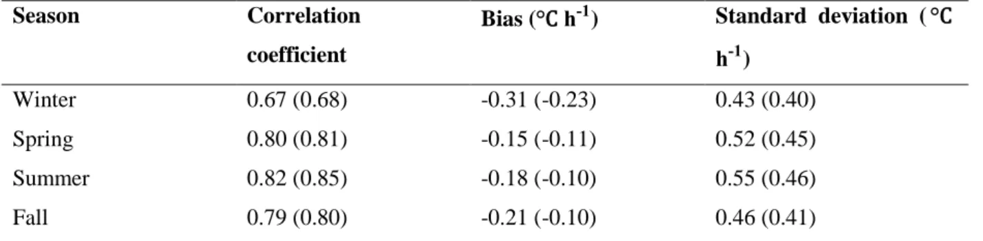
These statistics are estimated for each season as presented in Table 2. Correlation is high (0.82) and bias is low in summer. Nevertheless, the standard deviation remains high for this season, probably due to the higher values of temperature variation and the contribution of all terms involved for the summer in comparison to other seasons. For the spring and fall seasons, the correlation coefficient is still high (0.80). However, in winter the correlation coefficient is the lowest (0.67) with a higher bias (-0.31 °C h-1). Removing the extreme values of the observations and the model (i.e. taking the values that are within the 5th 200
and 95th percentile) gives better statistics (values in brackets in Table 2), confirming that the model encounters difficulties in reproducing these extreme events.
Figure 2d presents the hourly evolution of the five terms on the right side of Eq. (10), their sum (i.e. 𝜕𝑇2𝑚
𝜕𝑡 𝑚𝑜𝑑 in blue solid line)
and 𝜕𝑇2𝑚
𝜕𝑡 𝑜𝑏𝑠 (pink solid line) for the first days of September 2010. As expected, a diurnal cycle is identified for the radiative
(both cloud and clear-sky terms) and the heat atmosphere exchange terms. For the radiative terms, it is quite expected to have 205
a positive (negative) contribution during daytime (nighttime) due to the presence (absence) of solar radiation. In addition, there are some days when RCL (dotted red lines) plays an important modulating role in temperature variations, noticed during the
day on September 6th and 8th, when clouds manage to provide a maximum cooling effect of -2.9 °C h-1.
Evaporation and thermal conduction at the surface increase as the day goes on and the larger these terms are the more they will prevent the increase in temperature linked to the sensible and latent turbulent fluxes. But overall the temperature increases 210
during the day when these fluxes increase. However, the atmospheric heat exchange term (HA) is on average a negative contribution to temperature variations in one hour when Flat and Fsens increase in the afternoons. This negative contribution
could be mostly associated with the mixing of masses of air at the top of MLD, where depending on the state of temperature inversion, 𝑇𝑀𝐿𝐷 is likely to be very negative and this cold air could cool the surface. When RCL presents an important
contribution, HA becomes weaker and its diurnal cycle is attenuated due to the absence of solar radiation and hence fewer 215
surface fluxes are developed. The ground heat exchange and the advection terms play a minor role at this time scale and contribute negligibly to the model without a significant diurnal cycle detected.
Finally, the model follows well the observations, with a better agreement for daytime than for night-time, and with a better correlation for the first case (not shown). Reasons that may explain the bias are 1) the limited availability of 𝑇𝑀𝐿𝐷 data which
is estimated using only two radiosoundings per day and not hourly continuous values and 2) the hypothesis and assumptions 220
in some variables and atmospheric conditions outlined in the Appendix. Further, the temperature variations at night might be hard to quantify accurately due to the minor contribution of each of the non-radiative terms, for which contributions are close to zero, especially for the HA term, and where Flat and Fsens are most of the time very low (Section 3.3).
3.3 Annual- and Monthly-hourly cycles of the different terms
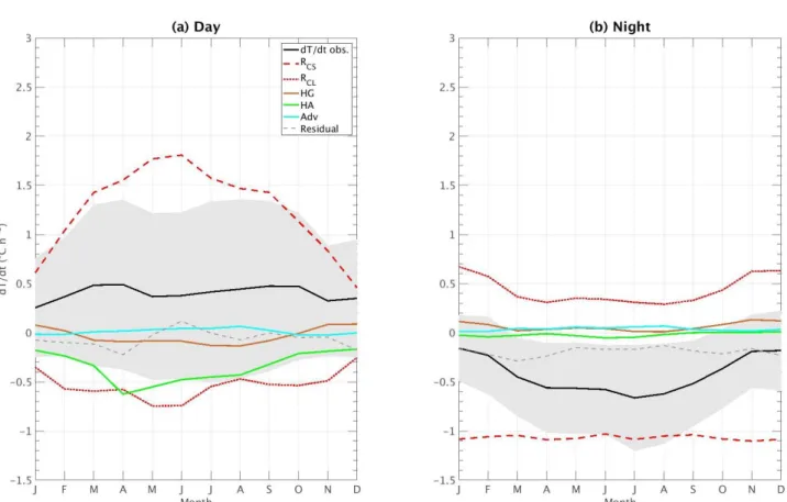
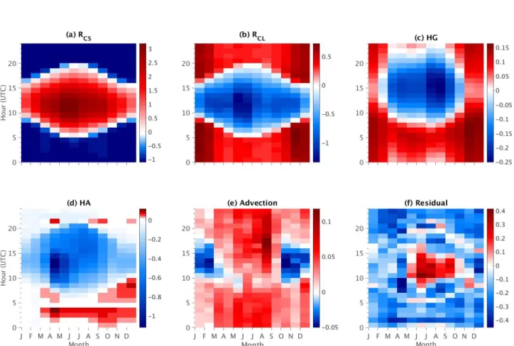
The mean contributions of each term are averaged monthly for both day and night (Fig. 3), whereas Figure 4 presents the 225
magnitudes of the monthly-hourly mean values from January 2009 to February 2014 of each term of the model. A residual term is calculated on these figures, which is calculated as the difference between the model (sum of all terms) and the observations (i.e. 𝜕𝑇2𝑚
𝜕𝑡 𝑚𝑜𝑑− 𝜕𝑇2𝑚
𝜕𝑡 𝑜𝑏𝑠).
According to Figure 3b and 4b for nighttime, the clear sky and cloud radiative forcing terms dominate in magnitude the hourly temperature variations at the surface and the other terms remain close to zero. Still during the night, 𝜕𝑇2𝑚
𝜕𝑡 𝑜𝑏𝑠 monthly mean is
230
negative throughout the entire year, with higher negative values during warm months than during winter. Indeed, RCL is always
positive during the night, and has an annual cycle more pronounced than the other terms, having a stronger effect in the cold months, due to the increase in cloud cover, especially low-level clouds which enhance an increase of the downwards flux of LW radiation and whose effect gets weaker while approaching summer, due to the modification of the radiative effect of clouds for this season. This decrease of RCL in summer explains the
𝜕𝑇2𝑚
𝜕𝑡 𝑜𝑏𝑠 annual cycle during night.
235
A diurnal cycle is pronounced for all the terms (Figure 4). RCS contributes the most in magnitude to local temperature variations
during daytime (Figure 3a), and the other terms damp its effect by providing a negative contribution. Furthermore, all the terms are mainly driven by the solar radiation intensity during the day. The diurnal and annual cycles of the RCS (RCL) term are
important, by having a positive (negative) contribution during the day, mostly dominating the temperature variations at this scale (as stated in(Gaevskaya, 1962). The contribution of RCL on
𝜕𝑇2𝑚
𝜕𝑡 𝑜𝑏𝑠 during daytime is more important during May and
240
June, and finds its minimum for December and January, when the solar radiation is weak, thus preventing clouds to strongly reduce it. Further, a maximum negative (positive) contribution to temperature variations of RCL (RCS) is found during the late
mornings for all the months, cooling (warming) the surface with a maximum mean value of -1.3 °C h−1 (3.2 °C h-1) in May and June at 10:00 UTC and 11:00 UTC.
In addition, the HA term plays an important role in temperature variations for spring and fall seasons, when there is an increase 245
late morning and the afternoon, especially during spring, with an hourly maximum averaged contribution of -1.1 °C h-1. The difference between day and night for the HA term is the largest during these months when the MLD can reach high values in the afternoon due to increased turbulence. For winter, its contribution is minimal due to the low development of the MLD. This result is in contrast with the negative (and very low) contribution of the HG term, which is maximal in summer in the 250
afternoon with an average smaller value of -0.25 °C h-1 when the surface temperature is the highest and thus strengthens its cooling action during daytime. An opposite effect is found in winter when the ground is usually warmer than the surface, yielding to a positive contribution (Fig. 3a and 4c). The advection term does not present a strong monthly-hourly cycle compared to the other terms, although one can distinguish a positive action (still very low) to local temperature variations at all seasons except winter during daytime, as shown in Figure 3a and 4e.
255
Lastly, the residual, defined as the difference between the model (sum of all terms) and the observations (i.e. 𝜕𝑇2𝑚
𝜕𝑡 𝑚𝑜𝑑− 𝜕𝑇2𝑚
𝜕𝑡 𝑜𝑏𝑠), also has a seasonal variability and is mainly negative, but a minimum difference of -0.45 °C h -1
between the two
datasets is found in April around noon, which is related to the negative increase of the HA term at that time. This is due to the important absence of latent heat flux data especially for this month, which implies an increase in the bias when 𝜏𝑎 is estimated
(see Table 1 and Appendix A). Nevertheless, during the months when solar radiation is strong, the residual reaches positive 260
values (with a maximum value around 0.4 °C h-1) but remains a low overestimation. These values for the residual are low compared to the magnitudes of RCS, but it remains almost at the same order of magnitude as the RCL and HA terms and a good
correlation in a diurnal cycle approach is found. Generally, this hourly mean residual could also be due to the simplifications and assumptions made in the model, under-sampling and energy imbalance.
4 Weight of the different terms acting on temperature variations 265
In this section, a random forest evaluation (James et al., 2013; Manish, 2016; Brownlee, 2016; Loh, 2002) is carried out at different time-scales to estimate the relative weight (i.e. importance) of each term in temperature changes according to the hour, month or seasons.
4.1 General behavior
Here, the random forest method is used to establish which term dominates the temperature changes in the model (𝜕𝑇2𝑚
𝜕𝑡 𝑚𝑜𝑑)
270
during day and nighttime. This machine learning method consists of bootstrapped-aggregated decision trees, a method that combines and gathers together the results of these trees to construct more powerful prediction models. Since in the present study the model has already been constructed, one of its most impressive features is used, which consists of the ability to provide a fully nonparametric estimation of the importance of each term (or predictor) on the model. One of the main advantages of this method is that it allows covering not only the impact of each term individually in the model but also the 275
multivariate interactions with other predictors. Indeed, other approaches to estimation of predictor importance (e.g. simple squared marginal correlations method, squared standardized coefficients) do not give reliable results when the problem involves correlated predictors (Grömping, 2007). Additionally, this method is used as a result of the nonlinear relationship between each separated term and the model (not shown), which does not yield to an estimation and quantification on how each process at the surface affects the temperature variations, an approach suggested and used by Miller et al. (2017) who estimated 280
the response and importance of some surface processes (such as Flat and Fsens) to the forcing radiative terms in Summit,
Greenland.
The predictor importance estimate value is defined as the sum of the mean square error (MSE) of each term averaged over all decision trees used and normalized by the standard deviation taken over the trees. This principle consists of permuting the values of a term – predictor – in the decision trees where this term was left out-of-bag and assess how much worse the MSE 285
becomes after the permutation (James et al. 2013, Chapter 8). Thus, the larger this value, the more important the term. This importance estimation feature from the random forest method has been previously used to calculate the variable importance in different datasets for many applied problems in sciences or health fields for both regression and classification studies (e.g. Archer et Kimes 2008; Genuer, Poggi, et Tuleau-Malot 2012; Strobl et al. 2007).
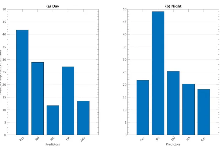
Figure 5a and b present the predictor (i.e. each term involved in 𝜕𝑇2𝑚
𝜕𝑡 𝑚𝑜𝑑, see Eq. (2)) importance estimate value for daytime
290
and nighttime respectively. Figure 5a corroborates that RCS is the most important term, followed by 𝑅𝐶𝐿 and then HA, whereas
HG is the least important term in the model developed for the timescale considered. Next, Figure 5b illustrates that 𝑅𝐶𝐿
dominates hourly temperature variations during nighttime, followed by HG and 𝑅𝐶𝑆. These results agree with(Kukla and Karl
(1993),)who suggested that the key regulator of nighttime warming temperatures is downward thermal radiation when cloudy cases are presented, an effect that is damped most of the time by the radiative cooling effect of the ground.
295
4.2 Diurnal cycle of the weights
The separation of daytime/nighttime does not allow the consideration of the importance of processes occurring during transition times of the diurnal cycle when the increase/decrease in temperature is the strongest. So, to better evaluate the influence of each term on hourly temperature variations at different times of the day, the importance estimation value is determined for each hour using the random forest method described previously in Section 4.1.
300
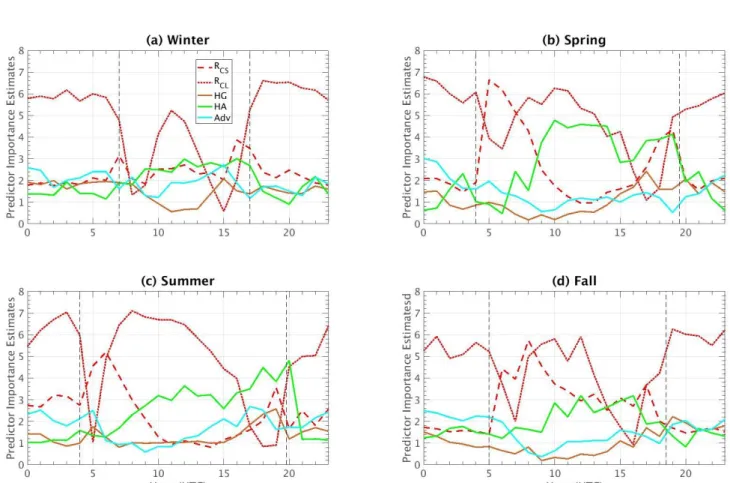
Figure 6 presents the results of this method for each season. As expected (and previously exposed), for all the seasons 𝑅𝐶𝐿 is
the term dominating during nighttime, just after sunset, and before sunrise (indicated by vertical dashed lines in black). After sunrise, the surface heating produced by the sun in the early morning enhances a high growth rate in the temperature variations, whose effect makes RCS the dominant term driving
𝜕𝑇2𝑚
𝜕𝑡 𝑚𝑜𝑑 at those hours of the day for all seasons, except for
winter. For this latter season (Figure 6a), the growth rate of RCS is almost the same as that of RCL and thus it does not expose
305
an important estimation value. This effect is due to the weak mean solar zenith angle (SZA) for this season, and the surface heating by the sun in clear-sky conditions is not strong enough to modulate temperature variations. On the contrary, RCL
importance reaches its minimum just after sunrise and before sunset, where, depending on the season, either 𝑅𝐶𝑆 or HA are the
main terms controlling temperature variations.
A shift in importance between RCL and RCS occurs during the rest of the day for the four seasons of the year. This effect is
310
explained by the variation of the data for these two terms: RCS standard deviation for a given hour/season is weak, and thus its
influence to explain the difference between one day to another at a specific hour remains minimal and it is not a strong predictor at diurnal cycle scale, especially in the summer and spring (Figure 6b and c, respectively) when other variables will modulate temperature variations. On the other hand, RCL turns into the main modulator of
𝜕𝑇2𝑚
𝜕𝑡 𝑚𝑜𝑑 for all the seasons due to its strong
standard deviation for a given hour/season, reaching its maximum importance in summer (Figure 6c). Therefore, the hourly 315
temperature variations are more sensitive to cloud changes rather than solar radiation which does not vary significantly for a specific hour from day to day.
Concerning the other terms, HA importance grows along the day. Its variation is greater than that of the other terms making it the second most important modulator most of the time (except for autumn, Figure 6d). Its contribution is weak in winter due to the lack of solar radiation and vegetation whose absence will diminish the turbulent heat fluxes measured at the surface, 320
along with a weak MLD. Note that it becomes sometimes the most important term in the late afternoon just before sunset. This is explained by an increase in instability of the ABL enhanced by a large boundary layer and surface temperature gradient (i.e. the difference between 𝑇𝑀𝐿𝐷− 𝑇2𝑚 reaches its maximum, see the third term of the right-side of Eq. (7)) in the late afternoon
(not shown) which is generated by the increase in turbulence fluxes near the surface.
Concerning the Adv term, it does not show a significant contribution during daytime but it becomes the second most important 325
modulator during nighttime before sunrise for all seasons except summer; probably a thermally-induced circulation linked to the urban heat island which is set up in Paris is at the origin of this importance: this circulation is likely to create a greater variation of temperature some nights when cooler air from rural areas is advected to warmer zones towards the city center. The SIRTA observatory, located in a suburban area at 20 km from the center of Paris could be indeed regularly affected by this modulation of circulation.
330
Figure 6 supports a clear and reliable estimation of the importance of each term split into seasons for every hour of the day, which is not seen by estimating the diurnal and annual cycle contribution of each term to temperature variations (cf. Section 3). Indeed, depending on the hour of the day (and thus the state of the atmosphere), one term will become important over the rest and temperature variations will be more sensitive to its change even if its contribution in terms of magnitude remains smaller compared to other terms. For instance, RCS absolute contribution during nighttime is higher than that due to RCL (Fig.
335
3b), and yet the latter is more important during nighttime due to its seasonal and hourly (not shown) contribution variability to
𝜕𝑇2𝑚
5 Discussion on the specific role of clouds on temperature variations
Section 4 shows that clouds are the main modulator of solar radiation on hourly temperature variations during the day (and the main contributor during the night). Knowing how each term affects the temperature variations and when they offset each other, 340
a deeper analysis is carried out in this section, to understand the role of clouds. This analysis is performed by considering other variables available in the SIRTA-ReOBS dataset to characterize both the atmosphere and the clouds.
In the following, only cloudy cases are considered. These cases are identified based on a criterion on the absolute value of CRE that must be higher than 5 W m-2 in SW and LW (Chiriaco et al., 2018) during daytime, whereas for nighttime only LW
is considered for this criterion. The SWCRE (and LWCRE) is calculating following Eq. (11): 345
𝑆𝑊𝐶𝑅𝐸 = 𝐹𝑆𝑊↓ − 𝐹𝑆𝑊,𝐶𝑆↓ (11)
According to this threshold, cloudy conditions correspond to 82% of the total cases from January 2009 to February 2014, and unique-clear-sky conditions represent the remaining 18%.
5.1 Daytime analysis
Since the RCS term dominates during daytime, the ratio of 𝜕𝑇2𝑚
𝜕𝑡 𝑜𝑏𝑠 divided by RCS is created to estimate how much these two
350
terms are driven by the solar radiation: when this ratio is close to 1, it means that the variations of temperature are the ones that would be expected in clear-sky conditions with no other modulators, and when this ratio deviates from 1 it means that the temperature variations are damped or enhanced by the other terms. The RCL/RCS ratio is also estimated, of which the
distribution (not shown) has two peaks, one between -0.5 and -1 and one slightly negative with a tail in positive values. Thus, three bins are created from the highest cooling effect to the warming effect: (i) −1.0 ≤𝑅𝐶𝐿
𝑅𝐶𝑆< −0.5 (bin 1), (ii) −0.5 ≤
𝑅𝐶𝐿 𝑅𝐶𝑆< 355
0 (bin 2) and (iii) 0 <𝑅𝐶𝐿
𝑅𝐶𝑆≤ 0.5 (bin 3). The cases with negatives or very close-to-zero values of RCS (10% of the cases), which occurred in early mornings and late afternoons, are excluded since they affect the sign of the distribution or give divergent values.
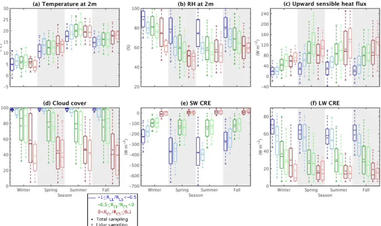
Figure 7a shows the values of the observed temperature variations divided by RCS and Figure 8 shows the distribution
(represented as box-and-whiskers) of different relevant meteorological observations available in the SIRTA-ReOBS dataset, 360
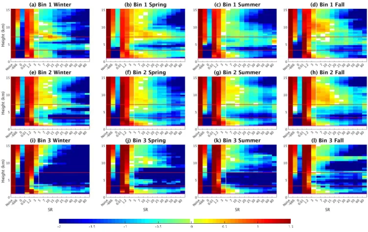
for each bin created, split into seasons for daytime. To add cloud information, lidar data are also considered but because they are not available all the time, and in particular when it is raining (see Sect. 2.2), they are presented as additional boxplots (light color ones) that correspond to the lidar sampling (whereas the dark color boxplots are for the total cloudy sampling). This difference of sampling mostly affects the first two bins when clouds have a cooling effect, for which both the occurrence and the amount of precipitations are the highest (not shown). Lidar SR(z) histograms presented in Figure 9 are estimated by 365
cumulating all lidar SR(z) observations available for one bin and one season in particular. The red horizontal lines on each histogram correspond to low- (P > 680 hPa), mid- (440 < P < 680 hPa), and high-level (P ≥ 440 hPa) clouds limits (Chepfer
et al. 2010; Chiriaco et al. 2018). Note that a Noise bin is presented here, which is simply the sum of the -999 and -777 bins that correspond to noisy and non-normalized profiles (cf. Section 2.2).
5.1.1 Case with strong cloud cooling effect - bin 1 370
Figure 7a shows that the values of temperature variations (normalized by RCS) are the lowest for clouds having the most
cooling effect (bin 1 in blue) for all the seasons. In winter this ratio stays mostly positive (temperature increase in one hour) but less than 0.5 (less than half the increase that could be reached if the sky was clear) and it can become negative during summer and fall, i.e. the warming induced by RCS can be counterbalanced by the clouds in these seasons. Besides, the cloud
cover is almost total and the radiative effects are strong, as seen in Figures 8d, e and f. In addition, the seasonal variability of 375
SWCRE is directly related to the seasonal variability of 𝐹𝑆𝑊,𝐶𝑆↓ , and not (or only slightly) to the seasonal variability of cloud
properties, since the ratio 𝑆𝑊𝐶𝑅𝐸 𝐹𝑆𝑊,𝐶𝑆↓
⁄
remains almost constant during the entire year (not shown) and cloud cover presents the highest mean values (Fig. 8d).The light blue bin is the same as the dark one except for lidar sampling, i.e. for non-rainy cases exclusively. Indeed, lower RH values (Fig. 8b) favor lower precipitation occurrence (not shown), higher amount of Fsens (Fig. 8c), and higher (i.e. less
380
negative) values of SW CRE (Fig. 8e) for the lidar sampling compared to the total one. Logically, lower LWCRE is found for the lidar sampling. As expected, temperatures are higher for the lidar sampling for all the seasons except summer, as shown in Fig. 8a, along with a more frequent negative temperature variation (Fig. 7a). For this sampling that excludes rainy cases, both higher and lower values of SWCRE are found for spring rather than for summer (Fig. 8e): the minimal value is around ~ − 600 W m-2 for spring whereas for summer it is ~ − 500 W m-2 (a situation not captured by the total sampling where summer
385
has a lower value of SWCRE than spring). Figure 9b shows that low- and high-level clouds are more frequent for spring than for summer (Fig. 9c) and thus stronger negative values of SWCRE are found for spring. Then, the important presence of mid-level clouds with a high value of lidar SR(z) (> 80) spotted in summer in Fig. 9c are potentially at the origin of the strong negative values of SWCRE despite the very low presence of other clouds. In addition, despite the strong negative values of SWCRE for this bin for all seasons, surface temperatures are not so low (Fig. 8a), partly due to the high LWCRE values (Fig. 390
8f) that slightly dampen the strong SWCRE.
Some differences in cloud presence can be detected in Figures 9a-d for the first bin. For the fall season, the SR(z) histogram in Fig. 9c exhibits an important presence of high-level thin clouds (especially above 8 km), along with mid-level thick clouds. Figure 9b also presents an important presence of high-level clouds in spring but within a smaller vertical range (7 < z < 10 km) compared to fall. Indeed, these high-level clouds could correspond to cirrostratus or cirrocumulus which form when a mass of 395
warm air meets a mass of cold air, where the lighter warm air rises and could form these cirrus clouds, an event that occurs more often in the transition seasons, such as spring and fall. In addition, spring exhibits high amounts of low-level thick clouds (SR>40) that are not detected the rest of the year, which could correspond to the moments just before a storm is set. Indeed,
the highest amount of precipitation rates are found for this season (not shown) and the cloud cover minima in Fig. 8d for the lidar sample is 90% (the highest among the other seasons) and less clear-sky conditions are found (0.01 < SR(z) < 1.2). 400
5.1.2 Cases with weak cloud radiative effect: cooling or warming
When RCS becomes dominant with respect to RCL (bins 2 and 3), temperature variations are most of the time positive,
especially in winter (Fig. 7a). In comparison with the first bin, the air becomes drier (higher sensitive heat flux and lower RH, Figure 8(b) and (c)), which agrees with less cloud cover (Fig. 8d), and lower LWCRE and less negative SWCRE (Fig. 8e and f). Figure 9 shows fewer differences between bin 1 and bin 2 (RCL< 0) than between bin 2 and bin 3 (RCL> 0) because this
405
figure only considers non-rainy situations and in section 5.1.1. it is noted the important differences between the two samplings (total and non-rainy) for bin 1 for most of the variables. This difference between the two samplings is weaker for bins 2 and 3, despite its existence in winter and fall. Figure 9 is thus more representative of the full sampling for these two bins than it is for the first bin.
For the lidar sampling, LWCRE in winter and fall is slightly higher than for the two other seasons for the second bin (Fig. 8f). 410
This is partly due to the presence of high-level thin clouds (5 > SR(z) > 20), such as cirrus, detected in the histograms of SR(z) for this bin in Fig. 9e and h for these two seasons, which is slightly more than for spring and summer.
In bin 3, the absence of mid-level clouds and the lower occurrence of high clouds compared to bin 2 is obvious, while the difference for low-level clouds is not clear. This is consistent with lower LWCRE (Fig. 8f) but not necessarily with the very low values (i.e. close to zero) of SWCRE observed for bin 3 (Fig. 8e). The SWCRE values close to zero are explained by the 415
fact that most of the hours corresponding to this bin 3 coincide just after sunrise (not shown), when solar radiation is still weak, thus explaining that 𝐹𝑆𝑊↓ ≈ 𝐹𝑆𝑊,𝐶𝑆↓ . These low SW and LWCRE values for the lidar sampling also correspond to low mean
cloud cover (Fig. 8d) and thus a lower amount of clouds are detected by the SR(z) histograms (Figure 9i-l). Note that some of the SWCRE values are even positive, revealing that 𝐹𝑆𝑊↓ > 𝐹𝑆𝑊,𝐶𝑆↓ , an effect observed when the direct part of solar radiation
is not fully attenuated and when some diffuse radiation reaches the surface in addition to the direct flux, radiation which is 420
strengthened by scattering processes in clouds and atmospheric particles. This effect thus increases observed radiation beyond a respective clear-sky scenario, and it mostly happens in winter (but could occur the rest of the year) in early mornings and/or late afternoons hours when the solar elevation angle is weak (Stapf et al., 2020; Wendisch et al., 2019). This distribution towards early morning hours explains that despite the high values of the ratio between temperature variations and 𝑅𝐶𝑆 (Fig.
7a) and lower cloud cover and cloud effects, surface temperatures are not always maximal for this bin (these maximal 425
temperatures happen only for spring and fall).
5.2 Nighttime analysis
During nighttime, a similar procedure is followed to analyze and characterize different meteorological variables under different cloudy conditions. Since RCL is the term dominating and controlling temperature variations (Section 4) and since RCS is
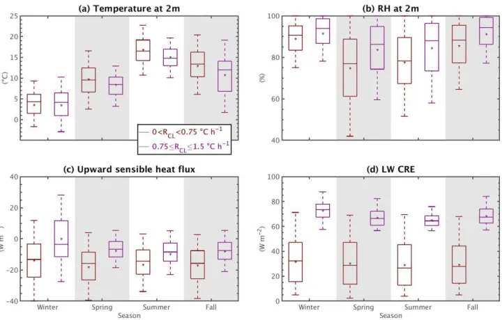
constant, it is not necessary to divide it by RCS. Thus, two bins are created from the PDF of 𝑅𝐶𝐿: 0 < RCL< 0.75 °C h−1 and
430
0.75 ≤ RCL≤ 1.5 °C h−1. During nighttime there is no SW radiation so clouds always have a warming effect on surface
temperature. The distribution of 𝜕𝑇2𝑚
𝜕𝑡 𝑜𝑏𝑠 for the two bins created for all the seasons is presented in Fig. 7b. Figure 10 shows
the same meteorological variables shown in Fig. 8 but for nighttime cases. Cloud fraction profiles are not shown because the lidar does not operate during nighttime.
Figure 7b shows that the temperature variations are generally stronger for the first bin than for the second bin, i.e. the negative 435
temperature variations induced by longwave cooling during nighttime are damped when the effect of clouds is stronger. This agrees with what is expected since, at hourly time scales, clouds are the most important factor in modulation of temperature variations during nighttime (see section 4). As expected, the second bin has stronger LWCRE values (Fig. 10e). The effect of clouds seems enhanced when cool and moist air is present over SIRTA (Fig. 10a, b). More details for each bin are given in the following subsection.
440
5.2.1 Case with weak cloud warming effect
For the first bin (0 < RCL< 0.75 °C h−1), LWCRE presents a wide range of values going from 5 W m-2 up to 75 W m-2 with
no seasonal variability detected (Fig. 10d), and yet temperatures are the highest for this bin (Fig. 10a) except in winter. As expected, upward sensible heat flux is most of the time negative due to surface cooling, as values of 𝜕𝑇2𝑚
𝜕𝑡 𝑜𝑏𝑠 are predominantly
negative (Fig. 10c and 7b, respectively), with drier air conditions since RH has the lowest values for all the seasons (Fig. 10b). 445
5.2.2 Case with strong cloud warming effect
The temperature distribution has the lowest values for all seasons (except spring) for the category of clouds that have the strongest warming effects (second bin, in purple on Fig. 10a). This category of clouds is tightly linked to strong LWCRE ranging from 55 W m-2 up to 90 W m-2 (Fig. 10d). These low temperatures could be associated with situations when the incoming air masses are colder, which is linked to large-scale situations (Pinardi and Masetti, 2000; Wang et al., 2005). Note 450
that here hourly temperature variations are studied, and indeed on multi-day time scales, it is the large-scale atmospheric processes that determine on the first order the daily temperature value.
Finally, the distribution of sensible heat flux is positive in winter with values reaching up to 40 W m-2 (purple box plot, Fig. 10c). These unusual and positives values during nighttime are explained by the presence of a strong stable atmospheric layer, where surface temperatures are the lowest except for spring (Fig. 10a) and the atmosphere is warmer at higher altitudes since 455
clouds contribute to warming the most at this time, and therefore a positive upward sensible heat flux develops. Similar behavior was previously found by Miao et al. (2012) in Beijing also during nighttime in cloudy conditions, where sensible and latent heat fluxes were close to zero due to the presence of a stable atmospheric layer, especially in winter when the sensible heat flux is found to be slightly greater than the latent heat flux. Indeed, almost half of temperature variation values are found to be positive for this season, as illustrated in Fig. 7b, and along with the positive upward sensible heat flux found, higher 460
temperatures are found for this bin which is not seen in the other seasons where the sensible heat flux is close to zero or mostly negative and temperatures are higher for the first bin (cloud with a low warming effect).
6 Conclusions
The European climate and most temperature anomalies are affected not only by the circulation of large-scale air masses (such as the NAO or blocking regimes) but also by smaller-scale processes such as cloud radiation and surface-atmosphere 465
interactions located within the atmospheric boundary layer. In this paper, a method is developed and evaluated to quantify each process that affects hourly 2 m-temperature variations on a local scale (near Paris), based almost exclusively on observations. The method exhibits good accuracy and is able to quantify well the realistic diurnal and monthly-hourly cycles of each term involved, especially in summer where statistics are the best. The clear-sky radiative term represents the biggest positive (negative) contribution during daytime (nighttime) with values reaching up to 4 ° h-1 (-1.7 ° h-1), whereas clouds cool 470
(warm) up to -3.7 ° h-1 (1.4 ° h-1). The atmospheric heat exchange becomes predominant in the late afternoons when turbulent fluxes develop due to the increase in atmospheric instability. Some of the biases found are due to the difficulty of the model to well reproduce smaller-scale processes such as the cold pool events.
The use of a random forest analysis makes it possible to identify which term dominates over the others. Clear-sky radiation most influences the 1-hour temperature variations during the day, whereas it is the cloud radiation during the night followed 475
by the ground heat exchange term. Nevertheless, separating the dataset into hours and seasons shows that the cloud radiation effect becomes predominant in several hours for all the seasons because it presents a greater variation of its hourly values than the clear sky radiative effect, especially in spring and summer during daytime when more local cloud cover variability occurs. This cloud dominance is still found despite the fact that the clear-sky radiation magnitudes are the highest on a monthly-hourly scale. Temperature variation is then more sensitive to cloud changes within an hour rather than the large contribution of clear-480
sky radiation which mostly dominates the early mornings when surface heat fluxes are not yet developed. The other terms remain important as there are times when some of them modulate temperature variations, especially the turbulent heat fluxes in the late afternoons. These terms also remain necessary to obtain the best coefficient estimator between the directly measured observations and the method developed.
To better understand the importance of clouds on temperature variations at this scale, a deeper analysis is performed partly 485
based on lidar profile observations. The atmosphere presents a high amount of cloud fraction detected by both the lidar and the sky imager during daytime which correlates well with the strong cooling contribution found for the cases when clouds have a strong cooling effect. Indeed, an important presence of mid-level thin and thick clouds is spotted for all the seasons (except spring) for these cases. These thick clouds could correspond to nimbostratus which are very opaque and often produce continuous moderate rain, but the lidar detects them just before the rain starts. Indeed, temperatures at this time are very low, 490
which contributes to these clouds forming since they usually form ahead of a warm front. On the contrary, a weak cooling effect is predominantly associated with low- and high-level thin clouds for all seasons. Situations with daytime positive cloud
radiative effect occur when the atmosphere is close to clear-sky conditions and corresponds to low- and high-level thin clouds mostly in early mornings and late afternoons. In addition, situations with weak cloud effect (either negative or positive) are associated with an important presence of high-level thick clouds for all the seasons (except winter), whose LWCRE is strong 495
but SW clear-sky radiation dominates and controls temperature variations along with other surface meteorological variables, high-level clouds which are more present than the times of strong cooling effect. Overall, a dominance of mid- and high-level clouds at the SIRTA observatory is detected for all cases. The dominant presence of this specific type of cloud is linked to the geographical position of the SIRTA observatory since it is located in a zone where warm and wet air coming from the Atlantic Ocean can nudge against the cold and dry masses of air coming from the Siberian region. This encounter of air masses (whether 500
it is the warm air that encounters cold air or the opposite) tends to form mostly high-level clouds. Similar behavior has been found by Chakroun et al. (2018) during nighttime and Mariotti et al. (2015) over the Euro-Mediterranean area where the variability of cloud fraction (CF) is driven mostly by the encounter of two different air masses coming from Northern Europe and Southern Africa. During nighttime, even when clouds have a positive important radiative effect, temperatures are low and they are more controlled by large-scale processes since surface turbulent fluxes are most of the time low and there is no 505
shortwave radiation. Since neither cloud fraction variable nor lidar data are available during nighttime, no information about the percentage of cloud presence can be known, yet variability on LWCRE is still found between clouds whose warming effect is weak and those whose warming effect is strong. This LWCRE variation is on the first-order controlled by the presence of clouds, but it could also be due to the sensitivity of LW radiation arriving at the surface to the presence of atmospheric gases and aerosols and not only to cloud radiative properties, as shown previously by Dufresne et al. (2002); Satheesh and Krishna 510
Moorthy (2005); Kushta et al. (2014). Besides, the strong stability of the atmosphere at night creates positive sensible heat flux when clouds have the warmest effect on temperature variations.
The approach developed in this study is innovative because it is predominantly based on observations. It opens several perspectives on the possibility for continuing work: (i) use of the approach in combination with weather regimes to better relate the small-scale processes to the large-scale atmospheric dynamics; (ii) application of the approach to other locations to 515
understand the spatial variability of the results and specific local conditions affect each of the terms involved in surface temperature variations; (iii) identification of the moments when one term becomes predominant over the rest by integrating the time into larger scales (such as weekly and monthly); and (iv) estimation of how well these estimations are represented in the present and future climate simulations to evaluate models and/or understand the evolution of the different terms in a warming climate. Further, the ground heat exchange contribution is very site-dependent (more than the other surface terms), 520
with different behavior in an urban environment, therefore it will be interesting to study its impact in the attenuation/amplification of maximum surface temperatures in periods of heatwaves.
Author contributions. OR carried out the data analysis, methodology and prepared all the figures. MC, SB and JR contributed
to the data analysis, advised on methods, validation and interpretation of results. OR wrote the manuscript with contributions 525
Acknowledgements. The authors would like to acknowledge Mesocentre ESPRI team at IPSL for providing storage resources
and giving access to SIRTA Re-OBS dataset, and also the SIRTA observatory for collecting and providing the geophysical variables and lidar data used in this study. The advection term as well as the temperature at the mixing layer depth were 530
estimated using Copernicus Climate Change Service Information ERA5 [2009-2014].
Competing interest. The authors declare that they have no conflict of interest.
535
References
Al-Hinti, I., Al-Muhtady, A., and Al-Kouz, W.: Measurement and modelling of the ground temperature profile in
Zarqa, Jordan for geothermal heat pump applications, Applied Thermal Engineering, 123, 131–137,
https://doi.org/10.1016/j.applthermaleng.2017.05.107, 2017.
Allan, R. P.: Combining satellite data and models to estimate cloud radiative effect at the surface and in the
540atmosphere, 18, 324–333, https://doi.org/10.1002/met.285, 2011.
Allan, R. P., Liu, C., Loeb, N. G., Palmer, M. D., Roberts, M., Smith, D., and Vidale, P.-L.: Changes in global
net radiative imbalance 1985–2012, Geophys Res Lett, 41, 5588–5597, https://doi.org/10.1002/2014GL060962,
2014.
Archer, K. J. and Kimes, R. V.: Empirical characterization of random forest variable importance measures,
545Computational Statistics & Data Analysis, 52, 2249–2260, https://doi.org/10.1016/j.csda.2007.08.015, 2008.
Arkin, P. A. and Meisner, B. N.: The Relationship between Large-Scale Convective Rainfall and Cold Cloud
over the Western Hemisphere during 1982-84, Mon. Wea. Rev., 115, 51–74,
https://doi.org/10.1175/1520-0493(1987)115<0051:TRBLSC>2.0.CO;2, 1987.
Arnold, N. S., Willis, I. C., Sharp, M. J., Richards, K. S., and Lawson, W. J.: A distributed surface
energy-550balance model for a small valley glacier. I. Development and testing for Haut Glacier d’ Arolla, Valais,
Switzerland, 42, 77–89, https://doi.org/10.3189/S0022143000030549, 1996.
Bastin, S., Chiriaco, M., and Drobinski, P.: Control of radiation and evaporation on temperature variability in a
WRF regional climate simulation: comparison with colocated long term ground based observations near Paris,
Clim Dyn, 51, 985–1003, https://doi.org/10.1007/s00382-016-2974-1, 2018.
555
Bennartz, R., Shupe, M. D., Turner, D. D., Walden, V. P., Steffen, K., Cox, C. J., Kulie, M. S., Miller, N. B., and
Pettersen, C.: July 2012 Greenland melt extent enhanced by low-level liquid clouds, Nature, 496, 83–86,
Brownlee, J.: Bagging and Random Forest Ensemble Algorithms for Machine Learning, Machine Learning
Mastery, 2016.
560
Chakroun, M., Bastin, S., Chiriaco, M., and Chepfer, H.: Characterization of vertical cloud variability over
Europe using spatial lidar observations and regional simulation, Clim Dyn, 51, 813–835,
https://doi.org/10.1007/s00382-016-3037-3, 2018.
Chen, T., Rossow, W. B., and Zhang, Y.: Radiative Effects of Cloud-Type Variations, 13, 264–286,
https://doi.org/10.1175/1520-0442(2000)013<0264:REOCTV>2.0.CO;2, 2000.
565
Chepfer, H., Bony, S., Winker, D., Cesana, G., Dufresne, J. L., Minnis, P., Stubenrauch, C. J., and Zeng, S.: The
GCM-Oriented CALIPSO Cloud Product (CALIPSO-GOCCP), 115, https://doi.org/10.1029/2009JD012251,
2010.
Cheruy, F., Campoy, A., Dupont, J.-C., Ducharne, A., Hourdin, F., Haeffelin, M., Chiriaco, M., and Idelkadi, A.:
Combined influence of atmospheric physics and soil hydrology on the simulated meteorology at the SIRTA
570atmospheric observatory, Clim Dyn, 40, 2251–2269, https://doi.org/10.1007/s00382-012-1469-y, 2013.
Cherviakov, M.: Variability of Earth’s radiation budget components during 2009 - 2015 from radiometer
IKOR-M data, 18, EPSC2016-9611, 2016.
Chiriaco, M., Bastin, S., Yiou, P., Haeffelin, M., Dupont, J.-C., and Stéfanon, M.: European heatwave in July
2006: Observations and modeling showing how local processes amplify conducive large-scale conditions, 41,
5755644–5652, https://doi.org/10.1002/2014GL060205, 2014.
Chiriaco, M., Dupont, J.-C., Bastin, S., Badosa, J., Lopez, J., Haeffelin, M., Chepfer, H., and Guzman, R.:
ReOBS: a new approach to synthesize long-term multi-variable dataset and application to the SIRTA supersite,
Earth Syst. Sci. Data, 10, 919–940, https://doi.org/10.5194/essd-10-919-2018, 2018.
Conangla, L., Cuxart, J., Jiménez, M. A., Martínez‐Villagrasa, D., Miró, J. R., Tabarelli, D., and Zardi, D.:
Cold-580air pool evolution in a wide Pyrenean valley, 38, 2852–2865, https://doi.org/10.1002/joc.5467, 2018.
ERA5: Fifth generation of ECMWF atmospheric reanalyses of the global climate .:
https://cds.climate.copernicus.eu/cdsapp#!/home, last access: 3 February 2020.
Dai, A., Trenberth, K. E., and Karl, T. R.: Effects of Clouds, Soil Moisture, Precipitation, and Water Vapor on
Diurnal Temperature Range, 12, 23, 1999.
585
Dewitte, S. and Clerbaux, N.: Measurement of the Earth Radiation Budget at the Top of the Atmosphere—A
Review, 9, 1143, https://doi.org/10.3390/rs9111143, 2017.
Dione, C., Lohou, F., Chiriaco, M., Lothon, M., Bastin, S., Baray, J.-L., Yiou, P., and Colomb, A.: The Influence
of Synoptic Circulations and Local Processes on Temperature Anomalies at Three French Observatories, J. Appl.
Meteor. Climatol., 56, 141–158, https://doi.org/10.1175/JAMC-D-16-0113.1, 2017.
Dufresne, J.-L., Gautier, C., Ricchiazzi, P., and Fouquart, Y.: Longwave Scattering Effects of Mineral Aerosols,
59, 1959–1966, https://doi.org/10.1175/1520-0469(2002)059<1959:LSEOMA>2.0.CO;2, 2002.
Gaevskaya, G. N., Kondrati’ev, K. Y., and Yakushevskaya, K. E.: Radiative heat flux divergence and heat regime
in the lowest layer of the atmosphere, Arch. Met. Geoph. Biokl. B., 12, 95–108,
https://doi.org/10.1007/BF02317955, 1962.
595Genuer, R., Poggi, J.-M., and Tuleau-Malot, C.: Variable selection using Random Forests, 11, 2012.
Grömping, U.: Estimators of Relative Importance in Linear Regression Based on Variance Decomposition, The
American Statistician, 61, 139–147, https://doi.org/10.1198/000313007X188252, 2007.
Haeffelin, M., Barthès, L., Bock, O., Boitel, C., Bony, S., Bouniol, D., Chepfer, H., Chiriaco, M., Cuesta, J.,
Delanoë, J., Drobinski, P., Dufresne, J.-L., Flamant, C., Grall, M., Hodzic, A., Hourdin, F., Lapouge, F.,
600Lemaître, Y., Mathieu, A., Morille, Y., Naud, C., Noël, V., O’Hirok, W., Pelon, J., Pietras, C., Protat, A.,
Romand, B., Scialom, G., and Vautard, R.: SIRTA, a ground-based atmospheric observatory for cloud and
aerosol research, Ann. Geophys., 23, 253–275, https://doi.org/10.5194/angeo-23-253-2005, 2005.
Hakuba, M. Z., Folini, D., Sanchez‐Lorenzo, A., and Wild, M.: Spatial representativeness of ground-based solar
radiation measurements, 118, 8585–8597, https://doi.org/10.1002/jgrd.50673, 2013.
605
Hartmann, D. L.: Chapter 6 Radiative Effects of Clouds on Earth’s Climate, in: International Geophysics, vol. 54,
Elsevier, 151–173, https://doi.org/10.1016/S0074-6142(08)60215-6, 1993.
Hartmann, D. L., Ockert-Bell, M. E., and Michelsen, M. L.: The Effect of Cloud Type on Earth’s Energy
Balance: Global Analysis., Journal of Climate, 5, 1281–1304,
https://doi.org/10.1175/1520-0442(1992)005<1281:TEOCTO>2.0.CO;2, 1992.
610Holtslag, A. a. M. and Van Ulden, A. P.: A Simple Scheme for Daytime Estimates of the Surface Fluxes from
Routine Weather Data, J. Climate Appl. Meteor., 22, 517–529,
https://doi.org/10.1175/1520-0450(1983)022<0517:ASSFDE>2.0.CO;2, 1983.
Ionita, M., Lohmann, G., Rimbu, N., and Scholz, P.: Dominant modes of Diurnal Temperature Range variability
over Europe and their relationships with large-scale atmospheric circulation and sea surface temperature anomaly
615patterns: VARIABILITY OF THE SEASONAL DTR, J. Geophys. Res., 117, n/a-n/a,
https://doi.org/10.1029/2011JD016669, 2012.
Ionita, M., Boroneanṭ, C., and Chelcea, S.: Seasonal modes of dryness and wetness variability over Europe and
their connections with large scale atmospheric circulation and global sea surface temperature, Clim Dyn, 45,
2803–2829, https://doi.org/10.1007/s00382-015-2508-2, 2015.
620