Relationships between GPS-signal propagation errors and EISCAT observations

HAL Id: hal-00316269

https://hal.archives-ouvertes.fr/hal-00316269

Submitted on 1 Jan 1996

HAL is a multi-disciplinary open access

archive for the deposit and dissemination of sci-entific research documents, whether they are pub-lished or not. The documents may come from teaching and research institutions in France or abroad, or from public or private research centers.

L’archive ouverte pluridisciplinaire HAL, est destinée au dépôt et à la diffusion de documents scientifiques de niveau recherche, publiés ou non, émanant des établissements d’enseignement et de recherche français ou étrangers, des laboratoires publics ou privés.

Relationships between GPS-signal propagation errors

and EISCAT observations

N. Jakowski, E. Sardon, E. Engler, A. Jungstand, D. Klähn

To cite this version:

N. Jakowski, E. Sardon, E. Engler, A. Jungstand, D. Klähn. Relationships between GPS-signal propagation errors and EISCAT observations. Annales Geophysicae, European Geosciences Union, 1996, 14 (12), pp.1429-1436. �hal-00316269�

Ann. Geophysicae 14, 1429—1436 (1996) ( EGS — Springer-Verlag 1996

Relationships between GPS-signal propagation errors

and EISCAT observations

N. Jakowski, E. Sardon, E. Engler, A. Jungstand, D. Kla¨hn

DLR e.V., Fernerkundungsstation Neustrelitz, Kalkhorstweg 53, Germany Received: 4 March 1996/Revised: 10 June 1996/Accepted: 11 June 1996

Abstract. When travelling through the ionosphere the signals of space-based radio navigation systems such as the Global Positioning System (GPS) are subject to modifica-tions in amplitude, phase and polarization. In particular, phase changes due to refraction lead to propagation er-rors of up to 50 m for single-frequency GPS users. If both the L1 and the L2 frequencies transmitted by the GPS satellites are measured, first-order range error contribu-tions of the ionosphere can be determined and removed by difference methods. The ionospheric contribution is pro-portional to the total electron content (TEC) along the ray path between satellite and receiver. Using about ten Euro-pean GPS receiving stations of the International GPS Service for Geodynamics (IGS), the TEC over Europe is estimated within the geographic ranges!20°4j440°E and 32.5°4/470°N in longitude and latitude, respec-tively. The derived TEC maps over Europe contribute to the study of horizontal coupling and transport proces-ses during significant ionospheric events. Due to their comprehensive information about the high-latitude ionosphere, EISCAT observations may help to study the influence of ionospheric phenomena upon propagation errors in GPS navigation systems. Since there are still some accuracy limiting problems to be solved in TEC determination using GPS, data comparison of TEC with vertical electron density profiles derived from EISCAT observations is valuable to enhance the accuracy of propagation-error estimations. This is evident both for absolute TEC calibration as well as for the conversion of ray-path-related observations to vertical TEC. The com-bination of EISCAT data and GPS-derived TEC data enables a better understanding of large-scale ionospheric processes.

Correspondence to: N. Jakowski

1 Introduction

Satellite radio beacon signals have been widely used in exploring the temporal and spatial structure of the iono-sphere since the launch of Sputnik I (e.g. Davies, 1991). Recently, space-based radio navigation systems such as the US Global Positioning System (GPS) offer new op-portunities for studying the ionosphere on a global scale (e.g. Coco, 1991; Wilson et al., 1995; Zarraoa and Sardon 1996). This is possible because GPS satellites transmit coherent dual-frequency signals in the L-band, low enough to measure a significant ionospheric contribution. On the other hand, the ionospheric refraction cannot be ignored at these frequencies in precise navigation and positioning systems. Single-frequency GPS users have to take into account ionospheric-induced propagation errors up to 50 m depending on the total electron content (TEC) along the ray path.

Although the first-order ionospheric effect can in prin-ciple be measured and therefore removed in dual-fre-quency satellite positioning systems by differencing measurements, there remain a number of unresolved ques-tions and problems related to the ionospheric behaviour; in particular, the auroral and polar ionosphere may cause severe distortions in GPS receivers (Bishop, 1994). So it is evident that EISCAT measurements and their interpreta-tion can help to improve the accuracy in satellite posiinterpreta-tion- position-ing. On the other hand, GPS measurements provide a powerful tool for large-scale ionospheric studies. If both observation areas overlap (see Fig. 1), direct correlation studies should be possible.

2 TEC measurements by means of GPS

GPS satellites transmit two coherent frequencies in the L-band at f1"1575.4 MHz (L1) and at f2"1227.6 MHz (L2). The L1 frequency is modulated by a public Coarse/ Acquisition code (C/A) with an effective wavelength of 300 m. Both carrier frequencies are modulated by a

Fig. 1. Scheme of the ray-path geometry between GPS satellites S1,2 and a receiver R. The mapping function M(e) is related to the zenith angle s of the ray path s at the pierce point with the assumed ionospheric shell at the height hsp

precise code (P or Y) with an effective wavelength of approximately 30 m. For unauthorized users the accuracy of GPS can be degraded by selective availability (SA) or antispoofing (AS). In case of SA, the accuracy obtained from the C/A code is limited to about 100 m by artificially introduced errors in the navigation message. If the encryp-ted Y code is turned on (AS), only military receivers can utilize the much more precise code measurements.

To determine the range between satellite and receiver, the time-delay of the pseudorandom-noise code sequences of the received signal is measured with rather high accu-racy by cross-correlation with the receiver-generated code sequence. However, these measurements are generally bi-ased by a number of errors, such as clock offsets on board satellites as well as on ground, tropospheric, ionospheric and multipath effects. So the measured ranges are referred to as pseudoranges p which may be written in the form:

p"o#c(dt!d¹ )#dI#dT#dMP#dq#dQ#ep, (1)

where o is the geometric range between satellite and receiver, c is the velocity of light in vacuum, dt is the offset of satellite clock, d¹ is the offset of receiver clock, dI is the ionospheric delay, dT is the tropospheric delay, dMP is the effect of multipath on pseudorange, dq is the instrumental group delay bias of the satellite, dQ is the instrumental group delay bias of the receiver andep is the random error on pseudorange.

When taking into account the refractive index of the ionospheric plasma at L-band frequencies the ionospheric contribution dI may be written as:

dI"fK2: neds, (2)

where ne is the electron density along the ray path s and

K"40.3 m3 s~1.

Since dI is frequency dependent, pseudorange differ-ences between L1 and L2 signals cancel out the unknown range o, the clock offsets and the tropospheric error in Eq. 1 and provide an expression for TEC": neds. But unfortunately the differential instrumental biases and multipath terms do not compensate. So the TEC

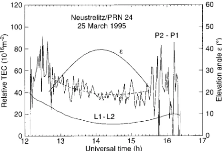
estima-Fig. 2. Differential measurements of pseudorange (p2!p1) and carrier phase (L1!L2) compared with the elevation angle (e). The smooth carrier phases are levelled to the noisy pseudorange phases for elevation angles greater than 20°

tion is strongly coupled with the estimation of instrumen-tal delays.

As shown in Fig. 2, the differential pseudorange signal

p2!p1 is strongly affected by multipath, especially at low

elevation angles. Since the fluctuations may exceed the expected TEC values, TEC estimations based only on pseudorange differences are rather uncertain.

The carrier phases can be described in a similar way as written in Eq. 1 for pseudoranges. However, due to their much shorter wavelength the multipath effect practically disappears, thus providing rather smooth data which are uncertain in absolute scale by multiples of wavelengths. To match the absolute level of the pseudoranges, the much more precise carrier-phase data are then adjusted by a constant. These levelled phase data are then used for further processing.

Assuming a second-order polynomial approximation for TEC over each receiving GPS station, the differential instrumental biases and TEC are estimated by means of a Kalman filter (Sardon et al., 1994) during a 24-h run for each satellite-receiver combination. During this time the biases are assumed to be constant.

This TEC estimation procedure reveals TEC data measured along permanently changing satellite links. To obtain normalized data, the slant TEC4 data are converted to the vertical TEC7 data by a mapping function M(e) which is in general defined by:

M(e)"TEC4/TEC7. (3) For a single-layer approximation of the ionosphere (Fig. 1) we obtain:

M(e)" 1

S

A

rE#hsp

B

2, (4)

wheree is the elevation angle, rE is the Earth radius and

hsp is the height of the assumed ionospheric layer at the

subionospheric point SP. Taking into account simulation calculations with realistic electron density profiles, the

Fi g. 3. Example fo r tw o -h o u rl y co n st ru ct ed T E C map s o ver E u ro p e for averaged T EC dat a o f A p ri l 19 95. Th e appl ie d grey sca le ha s a st ep w idth o f 3 0] 10 15 m ~2

Fig. 5. TEC map and

corresponding EISCAT CP3 trace on 3 February 1100 UT. The TEC contour lines are denoted in 1]1015 m~2 and differ by 12]1015 m~2

Fig. 4. TEC reconstruction error distribution function for differ-ences between TEC-map values and TEC values measured by the GPS station Neustrelitz which does not contribute to the TEC maps. The analysis includes approximately 2000—3000 data points from March 1995

height hsp of the ionospheric shell is fixed at hsp"400 km. After reducing the measured slant TEC data to the verti-cal-electron-content data at the subionospheric points, regional TEC7 maps may be constructed. Following Jakowski and Jungstand (1994) this is done by combining a regional TEC model (NTCM1) with actual GPS measurements over Europe. The empirical TEC model is based on numerous Faraday rotation observations car-ried out at linearly polarized VHF signals transmitted by geostationary satellites such as ATS-6, SIRIO, SMS and GOES types (e.g. Jakowski and Paasch, 1984).

In correspondence with the subionospheric traces of GPS signals receivable at DLR Neustrelitz, the area in

view covers the geographic ranges 32.5°4u470°N and 20.0°4j460°E in latitude and longitude, respectively. The pixel size of the map grid is defined as 2.5°]5° in latitude and longitude, respectively, resulting in 272 grid points.

The NTCM1 model takes into account basic relation-ships between solar radiation and diurnal and seasonal variations according to:

TEC"+5 i/1 3 + j/l 2 + k/1 2 + l/1Hi(h)½j(d)¸k(u,j, h, d)S1(F10), (5) where Hi(h) denotes the diurnal variation, ½j(d) denotes the annual variation, ¸k(u,j, h,d) characterizes the solar zenith angle dependence and S1(F10) denotes the solar activity dependence. The corresponding 60 coefficients were determined by least square fits to the observational data with RMS deviations from monthly averages of 5]1016 m~2 over a full solar cycle.

Highest accuracy in regional TEC monitoring can be achieved by combining a qualified model with actual measurements. The developed mapping algorithm ap-proximates to the measured values in the vicinity of the subionospheric points, whereas at greater distances model values dominate. Using the rather dense network of geodetic receivers of the International GPS Service for Geodynamics (IGS) (e.g. Zumberge et al., 1994) in Europe, about 40—70 measuring points can be obtained for map-ping every 30 s. This enables the monitoring of rather dynamic ionospheric processes on large scales. Figure 3 illustrates the procedure by presenting a two-hourly map of the TEC distribution over Europe for monthly averaged TEC data of April 1995.

The accuracy of such TEC maps was checked by com-paring measured TEC7 data with the corresponding data

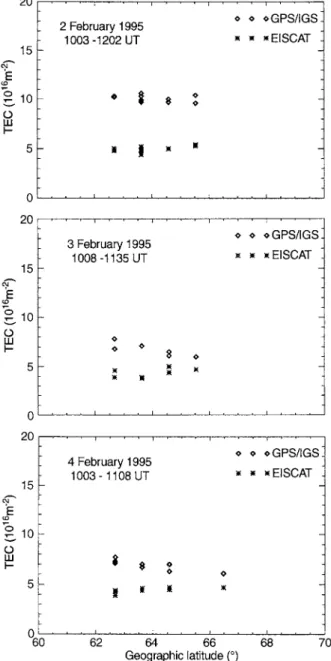
Fig. 6. Comparison of integrated and vertically mapped EISCAT CP3 data and TEC data derived from GPS measurements within 15-min time-intervals and 5° distance ranges between EISCAT and GPS measuring points

derived from TEC maps. When constructing the maps, the control data were excluded. As Fig. 4 demonstrates, the RMS error for TEC7 in March 1995 is in the order of 2]1016 m~2. This result is representative also for other stations. The achieved accuracy is high enough to study large-scale ionospheric processes even under low solar activity conditions.

3 Comparison of GPS-derived TEC with EISCAT data

Coordinated measurements of TEC by GPS and EISCAT should indicate a high correlation between incoherent-scatter-radar and TEC monitoring data in the

overlap-ping region. The incoherent-scatter-radar technique can provide a lot of information about all ionospheric layers. The most important parameters measured by EISCAT in different operation modes are the electron density, the plasma temperatures and ion drift velocities as a function of height. From these basic parameters a variety of further ionospheric parameters, such as ion composition, electric-field strength, winds and electric currents, can be deduced.

The Common Programme Three (CP3) measures the electron density at different latitudes between 62° and 78°N during a 30-min north-south scan. Since there is an overlapping region, these scans are well suited for com-parison with corresponding TEC monitoring data taken from the actual maps (Fig. 5). To compare the electron-density data measured by EISCAT with the total colum-nar electron content, the CP3 data are integrated from about 150- to about 500-km height and then mapped with

M(e) according to Eq. 4. It is evident that ionospheric

topside and plasmaspheric contributions are involved in GPS/TEC data but not in EISCAT measurements. Tak-ing into account electron densities of about 5]1010 m~3 near 150-km height at all selected days, the contribution of the bottomside ionosphere should be less than 4]1015 m~2.

Thus, the difference is expected to be mainly related to the topside ionosphere above 500 km including the plas-maspheric content. Since the plasplas-maspheric electron con-tent and its behaviour is not well known, a comparison between EISCAT and TEC-monitoring data can improve our knowledge about plasmasphere-ionosphere relation-ships especially at high latitudes. This is illustrated in Fig. 6 where height-integrated CP3 data are compared with the corresponding TEC data taken from the map along the CP3 scan trace. For the presentation in Fig. 6 only CP3 data with high-quality fits have been selected. During the considered measuring times subsequent scans have been included. This explains why at a fixed latitude several values with a small dispersion appear in the plot. The TEC data are deduced from subsequent TEC maps available every 10 min in such a way that the spatial distance between the EISCAT and GPS measuring points is less than 5° and these measurements are carried out within a 15-min interval. The corresponding EISCAT-CP3 trace for 3 February 1995 is shown in Fig. 5, illustra-ting that the map guides the EISCAT measurement by large-scale information about the horizontal structure for the ionospheric plasma.

The plots in Fig. 6 clearly indicate the contribution of the topside ionosphere and plasmasphere in the TEC data based on GPS measurements. Since the RMS mapping accuracy lies in the order of 2]1016 m~2 (cf. Fig. 4), estimations of the plasmashperic content are still rather crude. Nevertheless, large-scale perturbation processes and related magnetosphere-ionosphere coupling are ex-pected to be documented in the data.

The difference between TEC and EISCAT varies at the sample days 2—4 February 1995 between 1.5 and 5.5]1016 m~2, which seems to be quite reasonable. With

Ap values ranging from 23 to 26, the geomagnetic activity

Fi g. 7. Tw o -h o u rl y TE C map s d u ri n g a severe io no sp h eric st o rm o n 7 A pri l 1995 , (A p" 1 00) o ver Euro p e. T he appl ie d grey sc al e ha s a st ep w idth o f 3 0] 10 15 m ~2

TEC difference between EISCAT and GPS data might be related to geomagnetic perturbations. The convergence of the TEC data towards higher latitudes might be inter-preted by the natural reduction of the plasmaspheric con-tribution at high latitudes. The rather good agreement of GPS-derived TEC and EISCAT data confirms the accu-racy of the former. Since the TEC-estimation algorithms are based on some simplifying assumptions, the validation of the deduced TEC data products is an important task to which EISCAT effectively contributes.

4 Large-scale ionospheric perturbations

At high latitudes where significant interactions between the solar wind and the Earth’s ionosphere and atmosphere take place, the ionosphere is strongly influenced by pre-cipitating particles and by large-scale electric fields of magnetospheric origin. So a number of phenomena are generated in this region which may cause severe distur-bances in GPS receiving systems (e.g. Bishop et al., 1994).

In order to reduce signal degradation by ionospheric processes, a better understanding of the ionosphere and their relationships to the atmosphere and magnetosphere systems is required. In particular, the influence of signifi-cant short-term irregularities, detected as amplitude or phase scintillations, and strong large-scale variations of the plasma density should be studied in more detail. The combination of detailed EISCAT measurements with TEC maps of high temporal and spatial resolution should provide new insights into the complex behaviour of the ionosphere.

Although studied for more than six decades, iono-spheric storms are not yet fully understood. This is mainly due to the complex interaction of various processes in the magnetosphere, thermosphere and ionosphere on a global scale lasting several days. Experimental studies have to take into account this large-scale complexity. Regional or global maps of TEC in combination with other iono-spheric probing techniques such as EISCAT or vertical sounding are well suited to study some open questions related to the mechanism of ionospheric storms. Thus, for instance, the global response of the ionospheric ioniz-ation to electric fields or neutral winds may be studied effectively. If electric fields are assumed to play an impor-tant role during the onset phase of mid-latitude ionos-pheric storms (e.g. Jakowski et al., 1990, 1992), a simulta-neous increase in the ionospheric ionization (TEC) should be observed down to lower latitudes. Equatorwards-blow-ing winds or other propagatEquatorwards-blow-ing phenomena (AGW), which can contribute to the positive storm phase, need a few hours (e.g. Pro¨lss, 1995; Pro¨lss et al., 1991) to propagate to the equator, leading to a delayed increase in ionization along their way towards lower latitudes. As has been shown by Jakowski et al. (1992), EISCAT data pro-vide valuable information (electric fields, currents and atmospheric heating) to discuss ionospheric perturbation phenomena. Figure 7 provides two-hourly snapshots of the TEC over Europe on 7 April 1995. In the course of the geomagnetic storm on 6—7 April the geomagnetic activity

increased rapidly from Kp"0.3 (15—18 UT) on 6 April 1995 to 5.7 (03—06 UT) on 7 April 1995.

As Fig. 7 shows, the storm-induced ionization enhance-ment starts in the early morning of 7 April and leads to an increase in TEC over the whole latitude range in view (see also Fig. 3 for comparison). The excess production of ionospheric plasma in the auroral zone lasts up to about 2000 UT. Between 50 and 60°N, a well-pronounced elec-tron-density trough appears at the end of the positive phase around 2000 UT. The subsequent maps which are not shown here indicate a well-pronounced negative storm phase which moves from the auroral zone equator-wards. According to current theories this can be explained by an equatorward transport of composition changes con-sisting of an enrichment of N2 and O2 molecules (e.g. Pro¨lss, 1995; Pro¨lss et al., 1991). A more detailed discussion of such processes is beyond the scope of this paper.

5 Summary and conclusions

It has been shown that the coordinated analysis of GPS-derived TEC maps and simultaneously obtained EISCAT data can contribute both to improve positioning by GPS as well as to explore large-scale ionospheric processes. So the derived regional TEC maps over Europe can be validated by using EISCAT (especially CP3) data. Such TEC maps can be used in GPS navigation to reduce ionospheric propagation errors. EISCAT studies of small-scale and short-term irregularities contribute also to the understanding of ionospheric-induced GPS-signal degra-dations at high latitudes.

On the other hand, GPS-derived TEC maps with RMS accuracies of 2]1016 m~2 or better can effectively be used in studying large-scale ionospheric processes. Compar-ing the maps with correspondCompar-ing EISCAT observations, conclusions about the plasmaspheric content and plasmasphere-ionosphere coupling can be drawn. The combination of EISCAT data with TEC maps should be a powerful tool for studying ionospheric storms, to have a better understanding of generation mechanisms (EIS-CAT) and propagation processes (TEC map).

Acknowledgements. The authors express their deep thanks to the

colleagues from the IGS community who made available the high-quality GPS data sets. We thank also K. Schlegel for providing EISCAT data and E. Putz and P. Spalla for providing Faraday rotation data. The research was supported by the German Agency of Space Activities (DARA) under contract 50 Y19202.

Topical Editor D. Alcayde´ thanks R. Leitinger and another referee for their help in evaluating this paper.

References

Bishop, G. J., T. W. Bullett, and E. A. Holland, GPS Measurement of L-Band Scintillation and TEC in the Northern Polar Cap Ionosphere at Solar Maximum, Proc. Int. Beacon Sat. Symp. (Ed. L. Kersley), Aberystwyth, UK, 11—15 July 1994, pp. 29—32, 1994.

Coco, D., GPS-Satellites of Opportunity for Ionospheric Monitor-ing, GPS world, 47—50, October 1991.

Davies, K., Remote sensing of the ionosphere using satellite radio beacons, Indian J. Radio Space Phys., 20, 356—367, 1991.

Jakowski, N., and A. Jungstand, Modelling the Regional Ionosphere by Using GPS Observations, Proc. Int. Beacon Sat. Symp. (Ed. L. Kersley), University of Wales, Aberystwyth, 11—15 July 1994, pp. 366—369, 1994.

Jakowski, N., and E. Paasch, Report on the observations of the total electron content of the ionosphere in Neustrelitz GDR from 1976 to 1980, Ann. Geophysicae, 2, 501—504, 1984.

Jakowski, N., E. Putz, and P. Spalla, Ionospheric storm character-istics deduced from satellite radio beacon observations at three European stations, Ann. Geophysicae, 8, 343—352, 1990. Jakowski, N., A. Jungstand, K. Schlegel, H. Kohl, and K. Rinnert,

The ionospheric response to perturbation electric fields during the onset phase of geomagnetic storms. Can. J. Phys., 70, 575—581, 1992.

Pro¨lss, G. W., Ionospheric F-Region Storms, in Handbook of

Atmo-spheric Electrodynamics, Vol. 2, ed. Volland, CRC Press, Boca

Raton, Fla, 195—248, 1995.

Pro¨lss, G. W., L. H. Brace, H. G. Mayr, G. R. Carignan, T. L. Killeen, and J. A. Klobuchar, Ionospheric Storm Effects at Subauroral Latitudes: A Case Study, J. Geophys. Res., 96, 1275—1288, 1991.

Sardon, E., A. Rius, and N. Zarraoa, Estimation of the receiver differential biases and the ionospheric total electron content from Global Positioning System observations, Radio Sci., 29, 577—586, 1994.

Wilson, B. D., A. J. Manucci, and Ch. D. Edwards, Subdaily northern hemisphere ionospheric maps using an extensive network of GPS receivers, Radio Sci., 30, 639—648, 1995.

Zarraoa, N., and E. Sardon, Test of GPS for permanent ionospheric TEC monitoring at high latitudes, Ann. Geophysicae, 14, 11—19, 1996.

Zumberge, J., R. Neilan, G. Beutler, and W. Gurtner, The Interna-tional GPS-Service for Geodynamics—Benefits to Users., Proc.

ION GPS-94, Salt Lake City, September 20—23, 1994.

.