HAL Id: hal-02929614
https://hal.archives-ouvertes.fr/hal-02929614
Submitted on 3 Sep 2020
HAL is a multi-disciplinary open access
archive for the deposit and dissemination of
sci-entific research documents, whether they are
pub-lished or not. The documents may come from
teaching and research institutions in France or
abroad, or from public or private research centers.
L’archive ouverte pluridisciplinaire HAL, est
destinée au dépôt et à la diffusion de documents
scientifiques de niveau recherche, publiés ou non,
émanant des établissements d’enseignement et de
recherche français ou étrangers, des laboratoires
publics ou privés.
Distributed under a Creative Commons Attribution| 4.0 International License
atmospheric measurements: reliability of the uncertainty
estimates
G. Broquet, F. Chevallier, F.-M. Bréon, N. Kadygrov, M. Alemanno, F.
Apadula, S. Hammer, L. Haszpra, F. Meinhardt, J. Morguí, et al.
To cite this version:
G. Broquet, F. Chevallier, F.-M. Bréon, N. Kadygrov, M. Alemanno, et al.. Regional inversion
of CO2 ecosystem fluxes from atmospheric measurements: reliability of the uncertainty estimates.
Atmospheric Chemistry and Physics, European Geosciences Union, 2013, 13 (17), pp.9039-9056.
�10.5194/acp-13-9039-2013�. �hal-02929614�
Atmos. Chem. Phys., 13, 9039–9056, 2013 www.atmos-chem-phys.net/13/9039/2013/ doi:10.5194/acp-13-9039-2013
© Author(s) 2013. CC Attribution 3.0 License.
EGU Journal Logos (RGB)
Advances in
Geosciences
Open Access
Natural Hazards
and Earth System
Sciences
Open AccessAnnales
Geophysicae
Open AccessNonlinear Processes
in Geophysics
Open AccessAtmospheric
Chemistry
and Physics
Open AccessAtmospheric
Chemistry
and Physics
Open Access DiscussionsAtmospheric
Measurement
Techniques
Open AccessAtmospheric
Measurement
Techniques
Open Access DiscussionsBiogeosciences
Open Access Open Access
Biogeosciences
Discussions
Climate
of the Past
Open Access Open Access
Climate
of the Past
Discussions
Earth System
Dynamics
Open Access Open Access
Earth System
Dynamics
DiscussionsGeoscientific
Instrumentation
Methods and
Data Systems
Open Access
Geoscientific
Instrumentation
Methods and
Data Systems
Open Access DiscussionsGeoscientific
Model Development
Open Access Open Access
Geoscientific
Model Development
DiscussionsHydrology and
Earth System
Sciences
Open AccessHydrology and
Earth System
Sciences
Open Access DiscussionsOcean Science
Open Access Open Access
Ocean Science
DiscussionsSolid Earth
Open Access Open Access
Solid Earth
DiscussionsThe Cryosphere
Open Access Open Access
The Cryosphere
Natural Hazards
and Earth System
Sciences
Open Access
Discussions
Regional inversion of CO
2
ecosystem fluxes from atmospheric
measurements: reliability of the uncertainty estimates
G. Broquet1, F. Chevallier1, F.-M. Bréon1, N. Kadygrov1, M. Alemanno2, F. Apadula3, S. Hammer4, L. Haszpra5,6, F. Meinhardt7, J. A. Morguí8, J. Necki9, S. Piacentino10, M. Ramonet1, M. Schmidt1, R. L. Thompson11,*,
A. T. Vermeulen12, C. Yver1, and P. Ciais1
1Laboratoire des Sciences du Climat et de l’Environnement, CEA-CNRS-UVSQ, UMR8212, IPSL, Gif-sur-Yvette, France 2Servizio Meteorologico dell’Aeronautica Militare Italiana, Centro Aeronautica Militare di Montagna,
Monte Cimone/Sestola, Italy
3Research on Energy Systems, RSE, Environment and Sustainable Development Department, Milano, Italy 4Universität Heidelberg, Institut für Umweltphysik, Heidelberg, Germany
5Hungarian Meteorological Service, Budapest, Hungary
6Geodetic and Geophysical Institute, Research Centre for Astronomy and Earth Sciences, Hungarian Academy of Sciences,
Sopron, Hungary
7Federal Environmental Agency, Kirchzarten, Germany
8Institut Català de ciències del Clima, Barcelona, Catalonia, Spain 9AGH University of Science and Technology, Kraków, Poland
10ENEA, Laboratory for Earth Observations and Analyses, Palermo, Italy 11Max Planck Institute for Biogeochemistry, Jena, Germany
12ECN-Energy research Centre of the Netherlands, EEE-EA, Petten, the Netherlands *now at: NILU, Norwegian Institute for Air Research, Kjeller, Norway
Correspondence to: G. Broquet ([email protected])
Received: 8 February 2013 – Published in Atmos. Chem. Phys. Discuss.: 6 March 2013 Revised: 10 July 2013 – Accepted: 29 July 2013 – Published: 10 September 2013
Abstract. The Bayesian framework of CO2flux inversions
permits estimates of the retrieved flux uncertainties. Here, the reliability of these theoretical estimates is studied through a comparison against the misfits between the inverted fluxes and independent measurements of the CO2 Net Ecosystem
Exchange (NEE) made by the eddy covariance technique at local (few hectares) scale. Regional inversions at 0.5◦ resolu-tion are applied for the western European domain where ∼ 50 eddy covariance sites are operated. These inversions are con-ducted for the period 2002–2007. They use a mesoscale at-mospheric transport model, a prior estimate of the NEE from a terrestrial ecosystem model and rely on the variational as-similation of in situ continuous measurements of CO2
atmo-spheric mole fractions. Averaged over monthly periods and over the whole domain, the misfits are in good agreement with the theoretical uncertainties for prior and inverted NEE, and pass the chi-square test for the variance at the 30 % and
5 % significance levels respectively, despite the scale mis-match and the independence between the prior (respectively inverted) NEE and the flux measurements. The theoretical uncertainty reduction for the monthly NEE at the measure-ment sites is 53 % while the inversion decreases the stan-dard deviation of the misfits by 38 %. These results build confidence in the NEE estimates at the European/monthly scales and in their theoretical uncertainty from the regional inverse modelling system. However, the uncertainties at the monthly (respectively annual) scale remain larger than the amplitude of the inter-annual variability of monthly (respec-tively annual) fluxes, so that this study does not engender confidence in the inter-annual variations. The uncertainties at the monthly scale are significantly smaller than the sea-sonal variations. The seasea-sonal cycle of the inverted fluxes is thus reliable. In particular, the CO2sink period over the
European continent likely ends later than represented by the prior ecosystem model.
1 Introduction
Inverse modelling of CO2 surface fluxes consists of
assim-ilating atmospheric CO2 measurements in an atmospheric
transport model to retrieve the fluxes. The inversion systems also rely on prior statistical knowledge about the fluxes. This prior statistical knowledge typically consists of the compila-tion of estimates from vegetacompila-tion and ocean models, annual to hourly flux inventories and long-term flux climatologies with associated uncertainties. The inversion updates the prior estimate of the fluxes in order to decrease the misfits between the simulation of the CO2atmospheric mole fraction based
on this estimate and the actual CO2measurements at
atmo-spheric stations. The prior (posterior) misfits are caused by the combination of the prior (respectively posterior) uncer-tainties in the fluxes and by a series of other errors (gathered under the expression “observation errors”) which include the measurement errors, the transport model errors, and the dif-ferences between the time/space scales addressed by the in-version system and the scales of representativity of the mea-surements. Most inversion systems assume that all errors can be represented statistically using normal distributions. Their flux retrieval relies on the Bayesian framework, which, ac-counting for the prior uncertainty and the observation errors, describes the most likely estimate of the posterior fluxes with associated uncertainties.
The derivation of the uncertainty in the inverted fluxes is a strength of the Bayesian approach. However, it relies on the estimate of the statistics for the prior uncertainty and for the observation errors. There is a lack of independent data that could anchor and validate such statistics (Michalak et al., 2005; Gerbig et al., 2008; Chevallier et al., 2012). Therefore, a robust quantification of the posterior uncertainty remains challenging.
This study aims at evaluating the uncertainty estimates from an inversion system using comparisons with indepen-dent flux measurements, in the particular context of the inver-sion of the CO2Net Ecosystem Exchange (NEE) at high
res-olution over Western Europe, a region with one of the highest density of atmospheric and flux measurement stations. Three objectives underly this evaluation: increasing the confidence in the Bayesian estimate of uncertainties from inversion sys-tems challenged by inter-comparisons of results from dif-ferent inversion systems (Peylin et al., 2013), providing an objective approach for assessing the reliability of the uncer-tainty estimates based on independent data, and demonstrat-ing the high quality of results based on a regional inversion system for a relatively small region such as the European do-main considered in this study.
Broquet et al. (2011) (hereafter BR2011) developed a re-gional inverse modelling system based on a variational data assimilation framework (Chevallier et al., 2005) and on the atmospheric mesoscale transport model CHIMERE (Schmidt et al., 2001). They applied it to the inversion of the Eu-ropean CO2 NEE during summers 2002–2007 at 0.5◦ and
6 h resolution with prior estimates from the Organising Car-bon and Hydrology In Dynamic Ecosystems process-based model (ORCHIDEE) (Krinner et al., 2005) and with the assimilation of hourly in situ mole fraction data from the CarboEurope-IP (hereafter CE) atmospheric continuous sta-tions. They evaluated the results from the inversions by checking that the corrections applied by the inversions to the estimates from ORCHIDEE decreased the misfits to indepen-dent local flux measurements (at few hectares scale) from the CE eddy covariance flux towers during summer periods. Ob-viously, the inversion cannot solve the differences in space resolution between the model grid cells and the eddy covari-ance data nor the measurement error in these data (Hollinger and Richardson, 2005; Lasslop et al., 2008). However, the comparisons between the NEE estimates from the ecosystem or inversion model in the grid cells containing the locations of the flux towers and these measurements, both averaged over all flux tower locations in Europe and over 30-day pe-riods, showed significant decrease of the misfits and a better fit with the temporal variability of the data due to inversion.
This study applies the same system as BR2011 for a 6 yr long inversion of the European CO2NEE during the period
2002–2007 and extends their comparisons between the inver-sion based NEE and the eddy covariance data. The period of inversion is long enough in this study to gather enough sam-ples of monthly misfits between the eddy covariance mea-surements and the prior or posterior model NEE estimates, in order to derive robust statistics. These statistics are used here for evaluating the Bayesian uncertainty statistics of the inverse modelling system. Using the confidence in the uncer-tainties derived from such an evaluation, this paper also com-pares these uncertainties with the seasonal to inter-annual variations of the NEE in order to assess the reliability of the analysis of this variability in the inverted product. The rea-son is that the confidence in the inter-annual variability of NEE provided by state-of-the-art global atmospheric inver-sions is relatively low at a continental scale since there is a large spread of the results from different inversions, while these systems agree relatively well on the mean seasonal cycle of NEE in Europe (Peylin et al., 2013). Baker et al. (2006) estimated that the inter-annual variability of mean fluxes at the continental scales from existing global inver-sion systems was generally not significant due to uncertain-ties in the inverted fluxes. However, this conclusion did not apply to Europe, which gave some hope that the density of the observation network and the specificity of the transport over this continent could support a reliable estimate of the inter-annual variability. Therefore, the assessment of the re-liability of the seasonal to inter-annual variations of the NEE
G. Broquet et al.: Reliability of uncertainties from the inversion of CO2NEE 9041 −10 −5 0 5 10 15 20 35 40 45 50 55 BIS (120) CBW (200) CMN (2177) GIF (167) HEI (146) HUN (363) LMP (58) LMU (649) MHD (40) OXK (1185) PRS (3480) PUY (1475) SCH (1205) TRN (311) WES (12) JFJ (3580) KAS (1987)
Fig. 1. European domain and localisation of the CarboEurope IP atmospheric stations used for the inversion of NEE. The height of the stations is given in m a.s.l. between parentheses.
25
Fig. 1. European domain and localisation of the CarboEurope IP
atmospheric stations used for the inversion of NEE. The height of the stations is given in m a.s.l. between parentheses.
from the regional inversions aims at exploring whether the uncertainties from regional inversion reflect the spread of es-timates at global scale from Peylin et al. (2013) or whether state-of-the-art higher resolution inversion can significantly improve the estimate of the inter-annual variability.
The inverse modelling set-up is summarised in Sect. 2. The comparisons to eddy covariance measurements are detailed in Sect. 3 and analysed in Sect. 4. Finally the confidence in the analysis of the seasonal to inter-annual variability in the prior and inverted NEE is discussed in Sect. 5. Conclusions are given in Sect. 6.
2 Inverse modelling set-up
This section summarises the configuration of the inverse modelling system. More details and explanations about this set-up can be found in BR2011. Three-hourly prior estimates of the NEE from a simulation of the ORCHIDEE model are corrected with 6 h/0.5◦ resolution increments by the inver-sion system based on the assimilation of hourly averages of atmospheric mole fraction measurements at a series of sites: the Biscarosse (BIS), Cabauw (CBW), Monte Cimone (CMN), Gif-sur-Yvette (GIF), Heidelberg (HEI), Hegyhat-sal (HUN), Jungfraujoch (JFJ), Kasprowy Werch (KAS), Lampedusa (LMP), La Muela (LMU), Mace Head (MHD), Ochsenkopf (OXK), Plateau Rosa (PRS), Puy De Dôme (PUY), Schauinsland (SCH), Trainou (TRN) and Westerland (WES) CE continuous stations1 (see Fig. 1 and Table 1). Measurements from the period 2002 to 2007 are exploited here. The hourly data are selected for assimilation depending on UTC time and site altitude. Data from high altitude sta-tions (at locasta-tions higher than 1000 m a.s.l.) are assimilated
1http://ce-atmosphere.lsce.ipsl.fr/DATA_RELEASE/index.php?
p=ava
between 00:00 and 06:00 (UTC time is used hereafter) while other data are assimilated between 12:00 and 20:00 in order to avoid periods during which CHIMERE, like any regional transport model, bears large transport biases.
The CHIMERE model, denoted H, is used to simulate the atmospheric mole fractions and thus to compute the misfits to the atmospheric mole fraction measurements for a given es-timate of the NEE f . The configuration used for CHIMERE corresponds to a 0.5◦horizontal resolution, with 20 vertical layers and covers the domain 10.5◦W–22.5◦E 35–57.5◦N with ∼ 3.9 × 10⁶km2 of land surface. CHIMERE is driven by atmospheric mass fluxes from a simulation with the Penn State University/National Center for Atmospheric Research (PSU/NCAR) mesoscale model (known as MM5, Grell et al., 1994) that was nudged towards the operational analyses of the European Centre for Medium Range Weather Fore-casts (ECMWF). CO2anthropogenic emissions, ocean CO2
fluxes, and CO2atmospheric mole fractions at the lateral and
top boundaries of the domain are imposed to CHIMERE us-ing the same products as in BR2011. In particular, the bound-ary conditions are based on atmospheric mole fractions from the global inversion of Chevallier et al. (2010) that should ac-count for the large scale incoming transport of CO2from
op-timised fluxes outside the model domain or from opop-timised fluxes in the domain leaving the domain and re-entering it later.
The inversion system derives the statistically best esti-mate of the NEE f by minimising the sum J of the squared misfits to the hourly atmospheric mole fraction data yoand to the prior estimate of the NEE fb from the ORCHIDEE ecosystem model, weighted by their associated uncertainties, as a function of the 6 h/0.5◦resolution increments f − fb
to be applied by the inversion. Assuming that uncertain-ties have unbiased and Gaussian distributions, the misfits are weighted by the prior and observation error covariance matri-ces, B and R respectively, and the system minimises: J (f ) =
(f − fb)TB−1(f − fb) + (Hf − yo)TR−1(Hf − yo). The minimisation of J is handled iteratively using the M1QN3 algorithm (Gilbert and Lemaréchal, 1989). At each iteration, CHIMERE is used to estimate J and its adjoint HTis used to compute the sensitivity of the misfits between the measure-ments and the simulations to the NEE and thus ∇J . Uncer-tainties in the inverted NEE are derived using a Monte Carlo method which solves for the Bayesian estimate of the covari-ance of the posterior distribution as a function of B, R and H (see the end of this section for practical details).
The observation error R should account for all the sources of misfit between the model and the observations that are not adjusted by the inversion here, such as the transport and rep-resentativity errors, and the uncertainties in boundary condi-tions and in the anthropogenic emissions. Estimates of errors in mixing ratios at CE stations due to uncertainties in the an-thropogenic emissions are far lower than that of the transport and representativity errors (Peylin et al., 2011, BR2011) and they are ignored. Uncertainties in boundary conditions can
Table 1. CE atmospheric stations providing the CO2measurements used in this study.
Identifier CO2 Location Elevation Organisation Data time
Locality availability (ground level selection for
+ station height) inversion
BIS 2005–2007 −1.23◦E, 44.38◦N 73 m a.s.l. LSCE 12:00–20:00
Biscarosse +47 m a.g.l.
CBW 2002–2007 4.93◦E, 51.97◦N 0 m a.s.l. ECN, EEE-EA 12:00–20:00
Cabauw +200 m a.g.l. (top level)
CMN 2002–2003 10.68◦E, 44.17◦N 2165 m a.s.l. CAMM 00:00–06:00
Monte Cimone +12 m a.g.l.
GIF 2002–2007 2.15◦E, 48.71◦N 160 m a.s.l. LSCE 12:00–20:00
Gif sur Yvette +7 m a.g.l.
HEI 2002–2007 8.67◦E, 49.42◦N 116 m a.s.l. Univ. Heidelberg 12:00–20:00
Heidelberg +30 m a.g.l.
HUN 2002–2007 16.65◦E, 46.95◦N 248 m a.s.l. HMS 12:00–20:00
Hegyhatsal +115 m a.g.l. (top level)
JFJ 2005–2007 7.98◦E, 46.55◦N 3580 m a.s.l. Univ. of Bern 00:00–06:00
Jungfraujoch
KAS 2002–2007 19.93◦E, 49.23◦N 1987 m a.s.l. AGH 00:00–06:00
Kasprowy Werch
LMP 2002, 12.63◦E, 35.52◦N 50 m a.s.l. ENEA 12:00–20:00
Lampedusa 2005–2007 +8 m a.g.l. (top level)
LMU 2006–2007 −1.10◦E, 41.59◦N 570 m a.s.l. Univ. Barcelona 12:00–20:00
La Muela +79 m a.g.l. (top level)
MHD 2002–2007 −9.90◦E, 53.33◦N 25 m a.s.l. LSCE 12:00–20:00
Mace Head +15 m a.g.l.
OXK 2005–2007 11.81◦E, 50.03◦N 1022 m a.s.l. MPI-BGC 00:00–06:00
Ochsenkopf +163 m a.g.l. (top level)
PRS 2002–2007 7.70◦E, 45.93◦N 3480 m a.s.l. RSE 00:00–06:00
Plateau Rosa
PUY 2002–2007 2.97◦E, 45.77◦N 1465 m a.s.l. LSCE 00:00–06:00
Puy De Dôme +10 m a.g.l.
SCH 2002–2006 7.92◦E, 47.90◦N 1205 m a.s.l. Univ. Heidelberg 12:00–20:00
Schauinsland
TRN 2006–2007 2.11◦E, 47.96◦N 131 m a.s.l. LSCE 12:00–20:00
Trainou +180 m a.g.l. (top level)
WES 2002–2004 8.32◦E, 54.93◦N 12 m a.s.l. Univ. Heidelberg 12:00–20:00
Westerland
be a critical source of error in regional inversions (Göckede et al., 2010b; Lauvaux et al., 2012) and several studies at-tempted to adjust them using the inverse modelling frame-work (Peylin et al., 2005). Here, the potential error in the temporal and spatial variability in the concentrations from the global inversion that is used to apply the boundary con-ditions is ignored, but a general offset is applied before the inversion to cancel biases from the boundaries among other
sources of systematic errors (see below). Therefore, the ob-servation error R is set up with estimates of the CHIMERE configuration transport and representativity errors only.
Comparisons between simulated and measured radon con-centrations at HEI, GIF, PUY and MHD are used to de-fine the typical ratios between the transport and represen-tativity errors and the observed temporal variability in the hourly concentrations, and subsequently the transport and
G. Broquet et al.: Reliability of uncertainties from the inversion of CO2NEE 9043
representativity errors for CO2. Seasonal estimates of the
hourly errors (and thus of the hourly observation errors) are derived from the following definition of seasons (used here-after): winter = January–March; spring = April–June; sum-mer = July–September; fall = October–December. These es-timates are typically about 3.5 ppm at high altitude stations and at nighttime for any season. At the other stations, during the afternoon and evenings, they lie between 11 and 17 ppm during fall and winter (when vertical mixing is the lowest and thus when the model has difficulties in representing the vertical stratification close to the ground) or between 4 and 8 ppm in spring and summer.
Observation errors for different hours are assumed to be uncorrelated, which likely balances potential overestimations of the standard deviation (STD) for hourly errors when us-ing comparisons to Radon measurements (BR2011). There-fore, even though the configuration of observation errors for hourly data have a scale that is similar to that of the synop-tic variability in CO2 at the measurement sites, their
aver-ages at a daily scale are significantly smaller. Thus, the accu-racy of the comparison between the model simulations and the CO2 measurements is high enough to allow for
signif-icantly decreasing the uncertainties in the fluxes at a daily scale through the inversion.
Correlations in B are configured with values exponen-tially decreasing as a function of the lag between NEE times and space locations. Correlation e-folding lengths are set to 1 month and 250 km for prior uncertainties corresponding to a given 6 h window of the day (i.e., 00:00–06:00, 06:00– 12:00, 12:00–18:00 or 18:00–00:00), but prior uncertainties for different 6 h window of the day are not correlated. Like in the study of Chevallier et al. (2010), the STD in B is propor-tional to the heterotrophic respiration (using scaling factors derived so that daily uncertainties are similar to the ones di-agnosed by Chevallier et al., 2012). This STD is thus lower in fall and winter than in spring and summer, but a ceiling value is imposed for each 6 h window so that the daily uncer-tainty for a given 0.5◦×0.5◦grid cell remains smaller than
∼2.6 g C m−2day−1. This limits the differences between wintertime and summertime uncertainties with STD for un-certainties in 30-day mean NEE over the whole European domain ranging from 0.37–0.45 g C m−2day−1 in February to 0.54–0.58 g C m−2day−1in September.
One inversion is conducted for each one of the six years from 2002 to 2007. Before the inversions, a general offset (independent of the year, and for each 1 yr inver-sion, independent of space and time) is applied to the ini-tial and boundary conditions in order to remove the bias 1/nobsPni=1obs Hifb−yoi (where i is the index for the
dif-ferent CE data and Hiis the i-th line of H, i.e., the projection
into the time and space location of the i-th data) between the prior model atmospheric mole fractions and the whole set of
nobsCE data that will be assimilated from 2002 to 2007. This
bias originates from systematic errors in the boundary condi-tions, in the transport model and in the prior estimate of the
fluxes. The offset is needed to deal with this bias since the inversion system is configured to catch random errors only. Applying the same offset to all annual inversions prevents the system from adjusting the mean estimate of the NEE for the period 2002–2007, but the inversion can improve the es-timate of the seasonal to inter-annual variability in the NEE over Europe. Prior and posterior uncertainties are thus related to the estimate of the variations of the NEE around its mean value for 2002–2007.
The Monte Carlo estimate of the posterior uncertainties is based on ensembles of inversions with synthetic pseudo-random prior fluxes and observations (called Observing Sys-tem Synthetic Experiments, OSSEs) which, by construction, sample the prior uncertainty and the observation error, and, consequently, the Bayesian statistics for the posterior unctainty. These samplings converge towards the Bayesian er-ror statistics for a growing number of ensemble members. It is assumed that the uncertainty reduction (i.e., the rela-tive difference between the prior and posterior uncertainty) in monthly European NEE does not vary significantly from year to year or from one season to another. This assump-tion was checked by comparing the results from OSSEs that have been conducted for typical months of summer 2003 and 2006, for 2 weeks in December 2007 and for two weeks in July 2007. The results had a very small difference be-tween summer 2003 and 2006, or bebe-tween December and July 2007 (with less than 2 % difference in uncertainty reduc-tion) when considering the average over Europe, despite sig-nificant changes in the observation network (between 2003 and 2006), in prior and observation uncertainties (between July and December), in meteorological conditions (between all cases), and (consequently) in variances and spatial corre-lations of posterior uncertainties (between all cases), all these changes having opposed impacts that balance each others or that vanish when considering uncertainty reduction at the Eu-ropean and 15 to 30-day scale. The large cost of the compu-tations prevents building ensembles of OSSEs for the whole period of interest. Therefore, based on the assumption that the uncertainty reduction does not vary significantly for the NEE averaged at a European scale, the monthly estimate of posterior uncertainties in this paper (see Sect. 3.1 and Figs. 2 and 3) are all derived as the product of the monthly estimate of prior uncertainties (characterised by the B matrix) by the estimate of uncertainty reduction from the OSSEs for a typi-cal month during summer 2006. This uncertainty reduction is
∼60 % when considering the average of NEE over the whole European domain used here.
BR2011 give a discussion on the various sources of er-ror for such estimates of uncertainty reduction and of poste-rior uncertainties. This study, by assessing the reliability of the prior and posterior uncertainties, indirectly assesses the impact from these potential sources of errors. Posterior un-certainties in annual NEE could also be estimated based on ensembles of 1 yr long OSSEs. However, this has not been attempted due to the high computational cost that it would
2 4 6 8 10 12 Months −3 −2 −1 0 1 2 gC /m2 /da y
2002
−10 −5 0 5 10 15 20 35 40 45 50 55 2 4 Months6 8 10 12 −3 −2 −1 0 1 2 gC /m2 /da y2003
−10 −5 0 5 10 15 20 35 40 45 50 55 2 4 6 8 10 12 Months −3 −2 −1 0 1 2 gC /m2 /da y2004
−10 −5 0 5 10 15 20 35 40 45 50 55 2 4 Months6 8 10 12 −3 −2 −1 0 1 2 gC /m 2/d ay2005
−10 −5 0 5 10 15 20 35 40 45 50 55 2 4 6 8 10 12 Months −3 −2 −1 0 1 2 gC /m 2/d ay2006
−10 −5 0 5 10 15 20 35 40 45 50 55 2 4 Months6 8 10 12 −3 −2 −1 0 1 2 gC /m 2/d ay2007
−10 −5 0 5 10 15 20 35 40 45 50 55Fig. 2. Temporal evolution of monthly (i.e. 30-day mean) NEE (g C m
−2day
−1; negative values: sink) at the
CE-L4 locations specified for a full year in the maps. Blue: CE-L4 data averages; green: ORCHIDEE; red:
inverted fluxes; shaded areas: NEE ± standard deviation of the uncertainty in NEE.
26
Fig. 2. Temporal evolution of monthly (i.e., 30-day mean) NEE (g C m−2day−1; negative values: sink) at the CE-L4 locations specified for a full year in the maps. Blue: CE-L4 data averages; green: ORCHIDEE; red: inverted fluxes; shaded areas: NEE ± standard deviation of the uncertainty in NEE.
require, and due to the low confidence in the results derived at the annual scale (which is discussed in Sect. 4).
3 Comparisons to averages of eddy covariance measurements
3.1 Protocol and justification
Hourly data from the gap-filled CE-level 4 (CE-L4) prod-uct (Papale et al., 2006) are used to evaluate the inversions. These data are derived from the hourly averaging of
contin-uous quality controlled eddy covariance measurements from a large set of sites that are spread over the main regions and ecosystems of Europe. For the period 2002–2007, ∼ 45–50 eddy covariance sites have data in the CHIMERE domain (see the maps of Fig. 2 and Table 2).
In the following, the “misfits” refer to the differences be-tween the prior or posterior estimates of the NEE and the CE-L4 data averages. They are used in this paper to evaluate the “uncertainties” which hereafter refer to the estimates, in the inversion, of the prior uncertainty characterised by the B matrix, and of the posterior uncertainty based on the OSSEs. This evaluation relies on the fact that both the misfits and the
G. Broquet et al.: Reliability of uncertainties from the inversion of CO2NEE 9045 2 4 6 8 10 12 Months −3 −2 −1 0 1 2 gC /m2 /da y
2002
−10 −5 0 5 10 15 20 35 40 45 50 55 2 4 Months6 8 10 12 −3 −2 −1 0 1 2 gC /m2 /da y2003
−10 −5 0 5 10 15 20 35 40 45 50 55 2 4 Months6 8 10 12 −3 −2 −1 0 1 2 gC /m2 /da y2004
−10 −5 0 5 10 15 20 35 40 45 50 55 2 4 Months6 8 10 12 −3 −2 −1 0 1 2 gC /m 2/d ay2005
−10 −5 0 5 10 15 20 35 40 45 50 55 2 4 Months6 8 10 12 −3 −2 −1 0 1 2 gC /m 2/d ay2006
−10 −5 0 5 10 15 20 35 40 45 50 55 2 4 6 8 10 12 Months −3 −2 −1 0 1 2 gC /m 2/d ay2007
−10 −5 0 5 10 15 20 35 40 45 50 55Fig. 2. Temporal evolution of monthly (i.e. 30-day mean) NEE (g C m
−2day
−1; negative values: sink) at the
CE-L4 locations specified for a full year in the maps. Blue: CE-L4 data averages; green: ORCHIDEE; red:
inverted fluxes; shaded areas: NEE ± standard deviation of the uncertainty in NEE.
26
Fig. 2. Continued.
uncertainties can be used to statistically quantify the actual “errors” between the prior or posterior estimate of NEE by the inversion and the true NEE.
There are several sources of bias between eddy covariance measurements and model NEE during the period 2002–2007 which cannot be quantified. First, there can be annual biases in the eddy covariance measurements, due to imperfect data filtering and to gap-filling, which are large when compared to annual averages of the data, but, a priori, not when compared to monthly averages (Luyssaert et al., 2009; Lasslop et al., 2010). The weight of these biases for data averages is far larger than that of random measurement errors on individual data since the autocorrelation in time for these errors is
negli-gible (Lasslop et al., 2008). Eddy covariance sites often also show large sinks which are due to the regrowing nature of local ecosystems for many of these sites (Jung et al., 2011), while the actual sink should be smaller in the larger scale model grid cells which merge such regrowing ecosystems with near-equilibrium of disturbed ecosystems. Second, the analysis of the average of the inverted NEE over the whole period 2002–2007 is not sensible because of the application of a general offset to the concentrations before the inversion. The definition and the configuration of the inversion here is therefore dedicated to the estimate the variations of the NEE around its mean value for 2002–2007.
Table 2. CE eddy covariance sites providing the NEE L4 data used in this study.
Identifier NEE L4 data Location Site Responsible
Locality availability
ATNeu 2002–2004 11.31◦E, 47.11◦N Georg Wohlfahrt
Neustift Univ. Innsbruck
BEBra 2002, 4.52◦E, 51.30◦N Reinhart Ceulemans, Ivan Janssens
Brasschaat 2004–2007 Univ. Antwerp Wilrijk
BEJal 2006–2007 6.07◦E, 50.56◦N Luis Francois
Jalhay LPAP, Univ. Liège
BELon 2004–2007 4.74◦E, 50.55◦N Marc Aubinet
Lonzee GxABT, Univ. Liège
BEVie 2002–2007 5.99◦E, 50.30◦N Marc Aubinet
Vielsalm GxABT, Univ. Liège
CHOe1 2002–2003, 7.73◦E, 47.28◦N Ammann Christoph
Oensingen grassland 2006–2007 ART
CHOe2 2004–2007 7.73◦E, 47.28◦N Nina Buchmann
Oensingen crop ETH-Zuerich
CZBK1 2002–2007 18.53◦E, 49.50◦N Marian Pavelka
Bily Kriz forest CzechGlobe
CZBK2 2004–2006 18.54◦E, 49.49◦N Marian Pavelka
Bily Kriz grassland CzechGlobe
CZwet 2005–2006 14.77◦E, 49.02◦N Marian Pavelka
Czechwet CzechGlobe
DEGeb 2003 10.91◦E, 51.10◦N Werner Kutsch, Olaf Kolle
Gebesee vTI/MPI Jena
DEGri 2004–2007 13.51◦E, 50.94◦N Christian Bernhofer
Grillenburg TU Dresden – Meteorology
DEHai 2002–2007 10.45◦E, 51.07◦N Olaf Kolle, Alexander Knohl
Hainich MPI Jena/Univ. Goettingen
DEKli 2004–2007 13.52◦E, 50.89◦N Christian Bernhofer
Klingenberg TU Dresden – Meteorology
DEMeh 2003–2006 10.65◦E, 51.27◦N Axel Don
Mehrstedt vTI
DETha 2002–2007 13.56◦E, 50.96◦N Christian Bernhofer
Tharandt TU Dresden – Meteorology
DEWet 2002–2006 11.45◦E, 50.45◦N Corinna Rebmann, Olaf Kolle
Wetzstein MPI Jena
DKFou 2005 9.58◦E, 56.48◦N Joergen Olesen
Foulum DIAS
DKLva 2004, 12.08◦E, 55.68◦N Kim Pilegaard
Rimi 2006–2007 Risoe National Laboratory
DKSor 2002–2007 11.64◦E, 55.48◦N Kim Pilegaard
Soroe Risoe National Laboratory
ESES1 2002–2003 −0.31◦E, 39.34◦N Maria Jose Sanz
El Saler (Valencia) Fundaciòn CEAM
ESVDA 2004–2007 1.44◦E, 42.15◦N Arnaud Carrara
Vall d’Alinyà (Lleida) Fundaciòn CEAM
G. Broquet et al.: Reliability of uncertainties from the inversion of CO2NEE 9047
Table 2. Continued.
Identifier NEE L4 data Location Site Responsible
Locality availability
FRHes 2002–2007 7.06◦E, 48.67◦N André Granier
Hesse INRA Champenoux
FRLBr 2002–2005 −0.76◦E, 44.71◦N Denis Loustau
Le Bray INRA Pierroton
FRLq1 2004–2007 2.73◦E, 45.64◦N Katja Klumpp
Laqueuille intensive INRA Clermont
FRLq2 2004–2007 2.73◦E, 45.63◦N Katja Klumpp
Laqueuille extensive INRA Clermont
FRPue 2002–2007 3.59◦E, 43.74◦N Serge Rambal
Puechabon CEFE
HUBug 2002–2007 19.60◦E, 46.69◦N Zoltan Tuba
Bugac Eotvos Lorand Univ.
HUMat 2004–2006 19.72◦E, 47.84◦N Zoltan Tuba
Matra Eotvos Lorand Univ.
IECa1 2004–2007 −6.91◦E, 52.85◦N Mike Jones
Carlow crop Trinity College Dublin
IEDri 2003 −8.75◦E, 51.98◦N Gerard Kiely
Dripsey Univ. College Cork
ITAmp 2002–2007 13.60◦E, 41.90◦N Dario Papale
Amplero Univ. Tuscia Viterbo
ITCol 2002–2007 13.58◦E, 41.84◦N Giorgio Matteucci
Collelongo IEIF CNR
ITCpz 2002–2007 12.37◦E, 41.70◦N Dario Papale
Castelporziano Univ. Tuscia Viterbo
ITLav 2002–2003 11.28◦E, 45.95◦N Damiano Gianelle
Lavarone Fondazione E. Mach
ITLec 2005–2007 11.27◦E, 43.30◦N Lorenzo Genesio
Lecceto IBIMET CNR
ITLMa 2003–2004, 7.15◦E, 45.58◦N Fabio Petrella
La Mandria 2006 IPLA SpA
ITMal 2003 11.70◦E, 46.11◦N Antonio Raschi
Malga Arpaco IBIMET CNR
ITMBo 2003 11.04◦E, 46.01◦N Damiano Gianelle
Monte Bondone Fondazione E. Mach
ITNon 2002–2003 11.08◦E, 44.68◦N Franco Miglietta
Nonantola IBIMET CNR
ITPia 2002–2003 10.07◦E, 42.58◦N Vaccari Francesco Primo
Pianosa IBIMET CNR
ITPT1 2002–2004 9.06◦E, 45.20◦N Günther Seufert
Parco Ticino forest JRC
ITRen 2002–2007 11.43◦E, 46.58◦N Stefano Minerbi, Leonardo
Montagnani
Table 2. Continued.
Identifier NEE L4 data Location Site Responsible
Locality availability
ITRo1 2002–2007 11.93◦E, 42.40◦N Dario Papale
Roccarespampani 1 Univ. of Tuscia Viterbo
ITRo2 2002–2007 11.92◦E, 42.39◦N Dario Papale
Roccarespampani 2 Univ. of Tuscia Viterbo
ITSRo 2002–2007 10.28◦E, 43.72◦N Alessandro Cescatti
San Rossore JRC
NLCa1 2003–2007 4.92◦E, 51.97◦N Eddy Moors
Cabauw WUR
NLLan 2005–2006 4.90◦E, 51.95◦N Eddy Moors
Langerak WUR
NLLoo 2002–2007 5.74◦E, 52.16◦N Eddy Moors
Loobos WUR
NLLut 2006–2007 6.35◦E, 53.39◦N Eddy Moors
Lutjewad WUR
NLMol 2005–2006 4.63◦E, 51.65◦N Eddy Moors
Molenweg WUR
PLwet 2004–2005, 16.30◦E, 52.76◦N Janusz Olejnik
Rzecin (PolWet) 2007 Univ. Poznan
PTEsp 2002–2007 −8.60◦E, 38.63◦N Gabriel Pita
Espirra Univ. Técnica de Lisboa
PTMi1 2003–2005 −8.00◦E, 38.54◦N Joao Santos Pereira
Mitra II (Evora) Univ. Técnica de Lisboa
PTMi2 2004–2007 −8.02◦E, 38.47◦N Casimiro Pio
Mitra IV (Tojal) Univ. de Aveiro
SKTat 2005–2007 20.16◦E, 49.12◦N Dario Papale
Tatra Danielov Dom Univ. Tuscia Viterbo
UKAMo 2003, −3.23◦E, 55.79◦N Marc Sutton
Auchencorth Moss 2005–2006 CEH Edinburgh
UKEBu 2004–2007 −3.20◦E, 55.86◦N Marc Sutton
Easter Bush CEH Edinburgh
UKESa 2003–2005 −2.85◦E, 55.90◦N John Moncrieff
East Saltoun Univ. Edinburgh
UKGri 2005–2006 −3.79◦E, 56.60◦N John Moncrieff
Griffin Univ. Edinburgh
UKHam 2004–2005 −0.86◦E, 51.12◦N Matthew Wilkinson
Hampshire Forest research – EHSD
UKHer 2006 −0.47◦E, 51.78◦N Keith Goulding
Hertfordshire BBSRC
UKPL3 2005–2007 −1.26◦E, 51.45◦N Richard Harding
Pang/Lambourne forest CEH Edinburgh
G. Broquet et al.: Reliability of uncertainties from the inversion of CO2NEE 9049
As a consequence of these long-term bias sources, the NEE estimates from the models and from the data are shifted homogeneously in space and time so that their average over 2002–2007 and over all the locations of CE-L4 sites in Eu-rope is cancelled before the comparisons, and, thus, so that these comparisons are unbiased and focused on the sea-sonal to inter-annual variability. All the results provided in the following are based on the estimates of the differences between the NEE and its 2002–2007 and European mean. Luyssaert et al. (2012) estimates the mean value for the long-term carbon uptake by ecosystems in Europe to be
−0.12 ± 0.04 g C m−2day−1.
Figure 2 shows the averages over all the time and space locations when and where CE-L4 data are available during each 30-day period within the CHIMERE domain, of the prior and inverted NEE at 0.5◦ resolution and of the
CE-L4 data. The spatial averaging over the different CE-CE-L4 lo-cations in Europe and over 30-day periods is assumed to strongly decrease the random measurement errors in the CE-L4 data (Lasslop et al., 2008) as well as the differences of representativity between these data and the estimates from the model which should be high when considering individual CE-L4 measurements (at a scale smaller than 1 km2) and the corresponding 0.5◦×0.5◦model grid cells, but which are as-sumed to be random, uncorrelated between the different mea-surement sites and not fully correlated over time at a given site. This assumption is supported by the good fit obtained by BR2011 between inverted estimates of NEE and spatially averaged CE-L4 data despite large misfits at individual sites. However, the residual differences in representativity between the averages (i.e., the average of the differences at local and hourly scale) may be still significant.
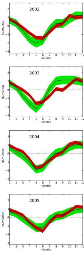
In a similar way, Fig. 3 shows the 30-day mean averages of the prior and inverted NEE over the whole CHIMERE domain in order to characterise the temporal variations of the European NEE in the light of the evaluation of the re-sults from the inversion at CE-L4 locations. In Figs. 2 and 3, the uncertainties provided for the averages of the prior NEE are those from the configuration for the B matrix in the in-version framework. The posterior uncertainties are based on the product of these prior uncertainties by the estimate of uncertainty reduction for the averages of NEE over CE-L4 locations (Fig. 2) or over 30-day and Europe (Fig. 3). The average of the six annual cycles at the monthly resolution for the whole CHIMERE domain is also displayed in Fig. 3. The knowledge of the correlations between uncertainties in monthly NEE from different years is needed to derive rigor-ously the prior or posterior uncertainties in the resulting av-erage NEE for a given month. Since there is no available esti-mate of the correlation of uncertainties from different years, the uncertainties in these monthly mean NEE for the period 2002–2007 are conservatively derived, based on the estimate of uncertainties obtained for specific years, and assuming full correlations between uncertainties in monthly NEE from year to year. 1 2 3 4 5 6 7 8 9 10 11 12 Months −3 −2 −1 0 1 2 gC /m 2/d ay
2002
1 2 3 4 5 6 7 8 9 10 11 12 Months −3 −2 −1 0 1 2 gC /m 2/d ay2003
1 2 3 4 5 6 7 8 9 10 11 12 Months −3 −2 −1 0 1 2 gC /m 2/d ay2004
1 2 3 4 5 6 7 8 9 10 11 12 Months −3 −2 −1 0 1 2 gC /m 2/d ay2005
1 2 3 4 5 6 7 8 9 10 11 12 Months −3 −2 −1 0 1 2 gC /m 2/d ay2006
1 2 3 4 5 6 7 8 9 10 11 12 Months −3 −2 −1 0 1 2 gC /m 2/d ay2007
1 2 3 4 5 6 7 8 9 10 11 12 Months −3 −2 −1 0 1 2 gC /m 2/d ay2002-2007 mean
Fig. 3. Temporal evolution of monthly (i.e. 30-day mean) NEE (g C m
−2day
−1; negative values: sink)
over the whole European domain of CHIMERE. Green: ORCHIDEE; red: inverted fluxes; shaded areas:
NEE ± standard deviation of the uncertainty in NEE. Dotted lines: NEE ± standard deviation of the variations
27
Fig. 3. Temporal evolution of monthly (i.e., 30-day mean) NEE
(g C m−2day−1; negative values: sink) over the whole European
domain of CHIMERE. Green: ORCHIDEE; red: inverted fluxes; shaded areas: NEE ± standard deviation of the uncertainty in NEE. Dotted lines: NEE ± standard deviation of the variations of NEE for a given month from 2002 to 2007.
9050 G. Broquet et al.: Reliability of uncertainties from the inversion of CO2NEE 1 2 3 4 5 6 7 8 9 10 11 12 Months −3 −2 −1 0 1 gC /m 2/d ay
2002
1 2 3 4 5 6 7 8 9 10 11 12 Months −3 −2 −1 0 1 2 gC /m 2/d ay2003
1 2 3 4 5 6 7 8 9 10 11 12Months −3 −2 −1 0 1 2 gC /m 2/d ay2004
1 2 3 4 5 6 7 8 9 10 11 12 Months −3 −2 −1 0 1 2 gC /m 2/d ay2005
1 2 3 4 5 6 7 8 9 10 11 12 Months −3 −2 −1 0 1 2 gC /m 2/d ay2006
1 2 3 4 5 6 7 8 9 10 11 12Months −3 −2 −1 0 1 2 gC /m 2/d ay2007
1 2 3 4 5 6 7 8 9 10 11 12 Months −3 −2 −1 0 1 2 gC /m 2/d ay2002-2007 mean
Fig. 3. Temporal evolution of monthly (i.e. 30-day mean) NEE (g C m
−2day
−1; negative values: sink)
over the whole European domain of CHIMERE. Green: ORCHIDEE; red: inverted fluxes; shaded areas:
NEE ± standard deviation of the uncertainty in NEE. Dotted lines: NEE ± standard deviation of the variations
of NEE for a given month from 2002 to 2007.
27
Fig. 3. Continued.
Figure 4 shows the distribution of all prior and posterior misfits between modelled and measured averages of NEE over 30 days and over CE-L4 locations from Fig. 2. The prior and posterior uncertainties from the inversion at the CE-L4 locations (which are shown in Fig. 2) vary from month to month and from year to year. Therefore, in principle, the es-timate of the STD of the misfits from Fig. 4 can only be used to check the quadratic mean (RMS) of the STD for these dif-ferent prior and posterior uncertainties only, i.e., to evaluate the STD of the mean distribution of the uncertainties. How-ever, the relative differences between these estimates of STD of the prior or posterior uncertainties in the monthly NEE at CE-L4 locations and their quadratic mean are smaller than 20 % most of the time, and are systematically smaller than
−1.5 −1.0 −0.5 0.0 0.5 1.0 1.5 gC m−2 day−1 0.0 0.2 0.4 0.6 0.8 1.0 1.2 1.4 1.6 [0. 1 g C m − 2 da y − 1] − 1 0.0 0.2 0.4 0.6 0.8 1.0
Fig. 4. Normalized distribution (bars, left axis) and cumulative distribution function (lines, right axis) of the
monthly misfits in NEE (g C m−2day−1) between ORCHIDEE (green) or the inverted NEE (red) and the CE-L4 averages from Fig. 2.
28
Fig. 4. Normalized distribution (bars, left axis) and cumulative
dis-tribution function (lines, right axis) of the monthly misfits in NEE
(g C m−2day−1) between ORCHIDEE (green) or the inverted NEE
(red) and the CE-L4 averages from Fig. 2.
2002 2003 2004 2005 2006 2007 −100 −50 0 50 100 gC m − 2 ye ar − 1
Prior anomalies at CE-L4 sites Posterior anomalies at CE-L4 sites CE-L4 anomalies
Prior anomalies for Europe Posterior anomalies for Europe
Fig. 5. Annual (i.e. 360-day mean) NEE anomalies to the 2002–2007 mean (g C m−2year−1; negative values: sink) at the CE-L4 locations specified in the maps of Fig. 2 and for the whole European domain.
29
Fig. 5. Annual (i.e., 360-day mean) NEE anomalies to the 2002–
2007 mean (g C m−2yr−1; negative values: sink) at the CE-L4
lo-cations specified in the maps of Fig. 2 and for the whole European domain.
30 % (this maximum value is reached by the relative differ-ence between the STD of the posterior uncertainty in January 2004 and the RMS of the posterior uncertainties in monthly NEE). According to these estimates from the inversion, the quadratic mean of monthly uncertainties is relatively close to the individual monthly uncertainties, and, therefore, the evaluation of this quadratic mean, based on comparisons to the STD of misfits to CE-L4 data, can be considered as an evaluation of individual monthly uncertainties.
Finally, Fig. 5 displays the annual anomalies to the 2002– 2007 mean in the CE-L4 data and in the prior and poste-rior estimates of the NEE in order to evaluate potential im-provements from the inversion bringing the estimate of the inter-annual variability of the NEE in closer agreement to
G. Broquet et al.: Reliability of uncertainties from the inversion of CO2NEE 9051
the CE-L4 data. However, the number of annual misfits (i.e., 6 prior misfits and 6 posterior misfits) is too low to get a reli-able sample of the statistics for the uncertainties in the annual anomalies of the NEE.
3.2 Results
The analysis of the prior misfits in Fig. 2 reveals differ-ences between ORCHIDEE and the CE-L4 data averages that are generally positive (i.e., that there is not enough uptake in the model) during spring and summer and negative (i.e., that there is not enough release of CO2 to the atmosphere
in the model) during fall and winter. These differences are even systematically positive in June–July and systematically negative from November to February. Values for these prior misfits exceed the monthly STD of the prior uncertainty for nearly 29 % of the months. This agrees very well with the assumption that the misfits have Gaussian distributions de-fined by the estimates of the prior uncertainties since 68 % of Gaussian distributions lies within one STD of their mean. The sampling of the prior misfits (Fig. 4) has a kurtosis and a skewness coefficients equal to −0.6 and 0.4 respectively, which also supports the assumption that the misfits and ac-tual errors follow a Gaussian distribution. However, Fig. 2 shows that the flatness of the distribution of the prior monthly misfits (seen in Fig. 4) is mainly due to the fact that positive values during spring–summer are generally larger than the negative values during fall–winter. The prior STD of monthly misfits is 0.64 g C m−2day−1 and should be compared with the value for the quadratic mean of the monthly prior uncer-tainties: 0.69 g C m−2day−1.
Figure 2 indicates that the inversion strongly decreases the misfits to CE-L4 data compared with the prior estimates. There are only 15 cases (out of 72) for which misfits are increased by the inversion (essentially during fall 2002 and summer–fall 2004). Unlike the prior misfits, the posterior misfits have a significant number of both positive and neg-ative values during all seasons. Consequently, the correlation between the monthly model estimates and the data is raised from 0.87 to 0.96 by the inversion, these high values being mostly due to the consistency of the seasonal cycles since these scores remain quite unchanged when removing annual means from the monthly estimates. During 2005–2007, the posterior misfits are smaller than the STD of the posterior uncertainties (except for 8 cases) but, due to larger values during 2002 and 2004 (regardless of the season), 37 % of these misfits exceed the monthly STD of the posterior un-certainty, which, again, agrees very well with the assumption that the misfits follow Gaussian distributions defined by the estimates of the posterior uncertainties. This assumption is also supported by the kurtosis and skewness coefficients of the sample of posterior misfits (Fig. 4) which are equal to 0.2 and 0.4 respectively, and by the value for the posterior STD which is equal to 0.4 g C m−2day−1, and thus, which is close to the value for the quadratic mean of the monthly
pos-terior uncertainties: 0.33 g C m−2day−1. The distribution of the posterior monthly misfits, which bears a weaker signature of seasonal variations than the prior distribution, has a small value for the kurtosis coefficient, which becomes positive af-ter inversion, showing that the inversion has been capable of applying stronger corrections in spring–summer when the prior had larger errors.
The uncertainty reduction for the NEE at the CE-L4 avail-able sites, defined by the relative difference between the quadratic means of the prior and posterior uncertainties in-tegrated over the location of the CE-L4 available sites for each year, is equal to 53 % (the relative difference between the estimate of the prior and posterior uncertainties based on the OSSEs varies from 48 % when integrated over the loca-tions of the sites in 2007 to 56 % when integrated over the locations of the sites in 2004). The reduction in the STD of the monthly misfits from the distributions in Fig. 4 is 38 %.
The comparison between Figs. 2 and 3 indicates that the seasonal variations of the prior and posterior NEE and the corrections from the inversion are qualitatively similar for the whole European domain and at CE-L4 locations. This is supported by the correlation between the prior (posterior) monthly NEE for the whole Europe and the prior (respec-tively posterior) monthly NEE at the CE-L4 locations which is 0.97 (respectively 0.98) and by the correlation between the corrections from the inversion for the whole of Europe and at the CE-L4 locations which is 0.88.
Misfits in the annual anomalies to the 2002–2007 mean are decreased by the inversion in 2002, 2003, 2006 and 2007, but increased in 2004 and 2005 (Fig. 5). The increase of the an-nual NEE (defining a positive NEE as a source of CO2) in the
data at CE-L4 sites each year from 2002 to 2006 is not sup-ported by the prior nor by the posterior estimates since these estimates identify strong positive anomalies in 2003 and in 2004, respectively. Actually, at the annual scale, prior or pos-terior misfits can be large compared to the typical anomalies given by the prior and posterior estimates or by the aver-ages of the data. These misfits are close to 80 g C m−2yr−1 in 2003 for the prior and in 2004 for the posterior while the largest anomaly given by the CE-L4 data is 63.4 g C m−2yr−1 in 2002. Furthermore, the estimate of the prior uncertainty in the annual anomalies at CE-L4 locations from 2002 to 2007 given by the set-up for the B matrix (using a 1-month correlation scale throughout each year) ranges from 110 to 130 g C m−2yr−1 which is systematically larger than all the misfits to the CE-L4 annual anomalies and systematically larger than all the model or data annual anomalies. Finally, the variations of annual anomalies from the prior and poste-rior estimates for the whole European domain are very differ-ent from that at CE-L4 locations. In particular, the posterior anomalies reach their maximum and minimum values during years that are different when considering the whole Europe and CE-L4 sites.
4 Discussion on the reliability of the estimate of uncertainties
4.1 Reliability of the estimate of uncertainties for the monthly means
Despite many potential sources of differences (explained in Sects. 2 and 3.1) between the STD of the misfits shown in Fig. 4 and the quadratic mean of the STD of the uncertainties from the inversions, comparing these two statistical quantifi-cations of the actual errors in the inverted NEE shows consis-tencies. The STD of the prior (posterior) monthly misfits is smaller (respectively larger) than the quadratic mean of the STD of monthly prior (respectively posterior) uncertainties at CE-L4 locations. However, the relative difference between the STD of the misfits and that of the estimates of the uncer-tainties by the inversion is only about 8 % for the prior NEE and 18 % for the posterior NEE. The results pass the chi-square test of the variance of the misfits sampling against the variance of the uncertainties with significance level of 30 % (for the prior sampling) and 5 % (for the posterior sampling). This gives a high confidence in the estimate of the STD for the monthly uncertainties and thus in the configuration of the inversions (in particular, the observation error along with that of the prior uncertainty).
Subsequently, the estimate of ∼ 53 % uncertainty reduc-tion from the inversion for monthly NEE at the CE-L4 sites is also relatively close to the reduction of STD of the monthly misfits (∼ 38 %), though larger, which was expected given the various sources of inconsistencies in the comparison listed in Sect. 3.1. This yields confidence in the estimate of ∼ 60 % uncertainty reduction for 30-day mean NEE over the whole CHIMERE domain from OSSEs during summers 2003 and 2006.
The analysis in Sect. 5 relies mostly on the estimate of pos-terior uncertainties. However, it can be noticed that according to the statistical results from this section and from Sect. 3.2, the assumption that the actual errors at a monthly scale are well characterised by the Gaussian distributions of the uncer-tainties from the inversion seems more robust for the prior estimates than for the posterior estimates, even though the shape of the sampling of posterior misfits is closer to that of a Gaussian distribution than that of the prior misfits.
4.2 Reliability of the estimate of uncertainties for the seasonal and annual means
The strong seasonal patterns in the prior misfits, with positive values in spring–summer and negative values in fall–winter, reveal seasonal errors (in the sense of actual differences with the true fluxes) in ORCHIDEE. Such large scale errors likely occur with such a model in which many processes underly-ing the NEE are driven with parameters relatively homoge-neous in space and time. In particular, the too simple mod-elling of crop phenology in the version of ORCHIDEE used
here (where crops are treated as a type of grass) likely yields an abnormally high positive NEE (a sink that is too small) during summer, especially during the heat wave of sum-mer 2003 (Smith et al., 2010b). It may induce high corre-lations between monthly uncertainties during a given season. On the other hand, the change of signs in the prior misfits from spring–summer to fall–winter suggests negative corre-lations between the uncertainties in prior monthly estimates from different seasons at CE-L4 sites even though they are far from occurring systematically at other flux measurement sites in the world according to Chevallier et al. (2012). This could be explained by the fact that in Europe, the ecosystem model, like actual ecosystems, balances its sink in spring– summer by its source during fall–winter to get an annual bud-get which is relatively close to equilibrium (compared to the typical fluxes in spring–summer or in fall–winter), and thus it may compensate a sink that is too small in spring–summer by a source that is too small during fall–winter. Therefore, the set-up of the correlations for daily prior uncertainties in NEE using values exponentially decreasing with 1-month correla-tion scale throughout each year may lead to significant errors in the estimate of the prior uncertainties at seasonal to annual scales in Europe even if the estimate of the prior uncertainties at monthly scale is good.
As explained in Sect. 2, this study has no estimate for the posterior uncertainty in NEE at the annual scale. The prior uncertainty in annual anomalies at CE-L4 locations is larger than the estimates of annual anomalies or than the prior or posterior misfits in anomalies. The comparisons between the inter-annual variability from the prior and posterior estimates and from CE-L4 data (Fig. 5) do not raise confidence in the prior annual anomalies nor in the corrections applied by the inversion to these anomalies. Therefore, these comparisons at the annual scale support the idea that the prior and poste-rior uncertainties in the annual anomalies are larger than the anomalies derived by the models. However, these compar-isons do not help evaluating typical values for these uncer-tainties. Furthermore, the inter-annual variations of the mod-els at CE-L4 sites do not seem representative of these varia-tions over the whole Europe. Finally, the potential annual bi-ases in the CE-L4 data due to filtering and gap-filling change from year to year, which bears consequences for the inter-annual variability of inter-annual budgets. Therefore, it seems dif-ficult to draw conclusions from the comparisons to CE-L4 data at the annual scale about the uncertainties in annual anomalies of the European NEE.
5 Reliability of the analysis of the seasonal to inter-annual variability
Section 4 yields confidence in the estimates of uncertain-ties in monthly NEE at CE-L4 sites and subsequently in the uncertainties in the monthly estimates of NEE at the Euro-pean scale. The significance of the seasonal to inter-annual
G. Broquet et al.: Reliability of uncertainties from the inversion of CO2NEE 9053
variations over Europe can thus be evaluated through com-parisons to the uncertainties provided at the European scale. The high correlation between the NEE or the corrections from the inversion between Figs. 2 and 3 indicate the good agreement between the variations in monthly estimates of the European NEE and the variations in the monthly estimates restricted to CE-L4 locations. The corrections to the seasonal and to inter-annual variations over Europe can thus also be evaluated by checking whether such variations are improved compared to that of the eddy covariance data averages at CE-L4 locations.
5.1 The seasonal cycle
The amplitude of the seasonal cycle provided by OR-CHIDEE is supported by the inversion. The monthly mean inverted NEE varies around its annual mean from ∼ −1.53± 0.23 g C m−2day−1in May to ∼ 1.1 ± 0.19 g C m−2day−1in November with differences between May and June or be-tween November and December that are smaller than the posterior uncertainties in European NEE (Fig. 3). The CE-L4 eddy covariance data also indicate minimum values in May– June and maximum values in November–December which, along with the high correlations between the monthly prior or posterior NEE and these data, gives confidence in the phase of the seasonal cycle from ORCHIDEE or from the inversion. As explained in Sect. 3.1, the long-term mean NEE (ac-tually the mean NEE for 2002–2007 and for the whole CHIMERE domain which is smaller than the one analysed in Luyssaert et al., 2012) has been set to 0 in the prior and pos-terior results from the inversion. Consequently, these results only reflect the variations around such a long-term mean, which could prevent assessing the sign of the value for full monthly NEE estimates. However, the typical estimate of the long-term mean NEE in Europe by Luyssaert et al. (2012), which is equal to −0.12 ± 0.04 g C m−2day−1(see Sect. 3.1), is smaller than the posterior uncertainties in monthly NEE. Considering the NEE for Europe that is obtained by adding this long-term mean estimate from Luyssaert et al. (2012) to the monthly variations around the 2002–2007 mean from the prior or posterior NEE of the inversions, the NEE based on the posterior anomalies should have a significantly (i.e., greater than the STD of the posterior uncertainty) negative value from April to July (in 2002, 2003 and 2005) or to August (in 2004, 2006 and 2007) while the NEE based on the prior anomalies, in general, should not be significantly negative from July. On average, the uptake should last from March/April to August considering the NEE estimate based on the sum of the anomalies from the inversion and the long-term mean from Luyssaert et al. (2012).
The significant positive increment in the NEE between July and September is the main pattern of the correction to the seasonal cycle from the inversion, which results in a more regular decrease in time of the uptake from June to Septem-ber. This regular decrease of the uptake during summer can
also be identified in the CE-L4 averages. The shape of the corrections and of the variations in monthly mean NEE from the inversion in 2003 fits well with that which were obtained independently by Smith et al. (2010b) who tested explicit crop modelling within ORCHIDEE, which raises additional confidence in the posterior estimate of the seasonal varia-tions.
5.2 The inter-annual variability of monthly to annual means
Since Sect. 4 raises confidence in the estimates of uncertain-ties in monthly NEE but not in annual NEE, the following analysis primarily focuses on the inter-annual variability of monthly means, but it also attempts at deriving insights on the robustness of the inter-annual variability of seasonal to annual means based on the results from Sect. 3.2.
The inter-annual variability of the monthly inverted NEE has a STD ranging from 0.07 g C m−2day−1 during Jan-uary to 0.22 g C m−2day−1in August while the STD for the posterior uncertainty is systematically (for every year and any month) higher than 0.15 g C m−2day−1, and higher than 0.19 g C m−2day−1from May to November (Fig. 3). The es-timate of the STD of the inter-annual variability for a given month here is based on 6 values only, but this figure still shows that the differences from year to year, that are ob-tained here, do not generally exceed the posterior uncertainty in individual monthly estimates. If the posterior uncertainties were fully correlated from year to year, they would not affect the estimate of the inter-annual variability, and the correla-tions of uncertainties for 1 yr lags cannot be estimated based on the experimental framework of this study. However, high correlations in posterior uncertainties from year to year are quite unlikely since increments to monthly estimates of NEE from the inversions are influenced by the variability of many inversion parameters such as the atmospheric transport. Fur-thermore, posterior misfits to eddy covariance data are highly variable from year to year (with, as stated in Sect. 3.2, a sig-nificant number of both positive and negative values every seasons), which invites to assume that correlations of poste-rior uncertainties from year to year are not close to 1. There-fore, the inter-annual variability of the monthly inverted NEE during 2002 to 2007 does not seem large enough compared to the posterior uncertainties so that it can be safely analysed. The impact of the posterior uncertainty for the inter-annual variability of the NEE can be highlighted in the estimates of NEE themselves at seasonal scale. In Fig. 2, the decrease in the misfits to CE-L4 averages in June–September from the inversion seems larger during 2003 than for other years. This larger decrease in the misfits can be problematic since it un-derlies an increase of the uptake during summer 2003 which yields a mean sink for June–September 2003 that is higher than the mean sink for 2002 and 2005. Such a higher sink during the heat wave in 2003 than during summers 2002 and 2005 is questionable even though the large positive anomaly
during summer 2003 in Europe characterised by Ciais et al. (2005) is not clearly reflected by annual anomalies in Europe from global atmospheric inversions (Peylin et al., 2013). This example suggests that the inter-annual variability in seasonal NEE is smaller than the large uncertainties that the seasonal NEE likely bears and thus, cannot be safely analysed as well. Finally, the prior uncertainty in annual NEE for the whole Europe (∼ 80 g C m−2yr−1) is far larger than the STD of the inter-annual variability in the inverted estimate of annual NEE (∼ 20 g C m−2yr−1, see Fig. 5). A tremendous reduc-tion of uncertainty in annual NEE from the inversion is not likely. Therefore, this confirms the indications from Sect. 4 that there is a low confidence in the posterior estimate of the inter-annual variability in annual NEE at CE-L4 sites, and subsequently for the European domain.
6 Conclusions
This paper compares flux uncertainties estimated by a re-gional atmospheric inversion system and actual misfits be-tween the retrieved NEE and eddy covariance data at the Eu-ropean/monthly scale. The flux derived from the atmospheric inversion are much closer to the flux measurements than the prior fluxes. In addition, there is a remarkable agreement be-tween the statistics of the estimated uncertainties and that of the distribution of the misfits, despite the differences in scale between the inversion system and the measurement represen-tativity, and despite the measurement errors in the validation data. These facts generate confidence in the configuration of the inversion.
The comparison between the theoretical uncertainties from the inversion and the actual misfits to local eddy co-variance measurements also raises confidence in the estimate of monthly NEE at the European scale and of their seasonal variations within the uncertainty bounds derived by the inver-sion. In particular, the correction of the NEE seasonal cycle in summer appears significant and is a robust result from the inversion. However, this study indicates that the inter-annual variability of the monthly NEE is difficult to monitor with the present set-up of the inversion as its amplitude is likely sim-ilar to the posterior uncertainty. Even though the uncertain-ties in 1 yr mean fluxes are not evaluated here, the analysis of the variations in annual anomalies puts into question the robustness of the inter-annual variability of 1 yr mean fluxes too. These conclusions regarding the confidence in the inter-annual variability of NEE in Europe from inversions is quite close to the one that can be derived from the inter-comparison by Peylin et al. (2013), even though the European domain de-fined in Peylin et al. (2013) is far larger than the one used here. The improvements of the estimates of NEE allowed by regional inversions do not seem large enough presently to overcome the difficulties encountered by the global atmo-spheric inversions for deriving the inter-annual variability at continental scale.
The characterisation of large scale errors in ORCHIDEE suggests that a combination of the estimates from such a model and those from independent sources of information such as inventories of the evolution of carbon pools e.g., for forests and croplands (Ciais et al., 2010a; Luyssaert et al., 2010) would yield a significantly better prior estimate of the NEE (with smaller prior uncertainties). Thus, the uncertainty reduction from the inversion using such a prior would be smaller. This illustrates that the analysis of the uncertainty reduction cannot be separated from that of the prior uncer-tainty in order to assess the potential of inverse modelling and of the atmospheric observation networks. This study raises confidence in scores of uncertainty reduction for monthly es-timates which may appear optimistic because the system as-similates data at ∼ 15 atmospheric stations only. This appar-ent discrepancy derives from the fact that these large scores are due for a significant part to the use of a NEE prior esti-mate based on a free ecosystem model only. Still, the poste-rior uncertainties provided by the inversion for monthly NEE indicate that the CE atmospheric network (or a similar one) achieves sufficient precision to constrain the NEE seasonal cycle.
Some remaining difficulties in characterising long-term sources of errors may explain the weak confidence in the inter-annual variability and in the derivation of the mean Eu-ropean uptake using a regional inversion system. Improving the prior estimate of the NEE using inventories, extending the periods of inversion, including more atmospheric stations from the Integrated Carbon Observation System (ICOS2) and applying a robust adjustment of the boundary conditions should lead to better estimates of the annual budgets and of their inter-annual variability.
Acknowledgements. We would like to thank Philippe Peylin,
Nico-las Viovy and Fabienne Maignan who have provided the simula-tions of ORCHIDEE. We also thank all the principal investiga-tors and scientists of the CarboEurope-Integrated Project for the atmospheric data used in this study, and in particular Ingeborg Levin (Universität Heidelberg), Attilio Di Diodato (Servizio me-teorologico dell’ Aeronautica Militare Italiana), Markus Leuen-berger (Universität Bern), Alcide Di Sarra (Agenzia nazionale per le nuove tecnologie, l’energia e lo sviluppo economico sostenibile), Xavier Rodó (Institut Català de ciències del Clima, Barcelona), Jošt Valentin Lavriˇc (Max-Planck-Institute for Biogeochemistry), and Zoltán Barcza (Eötvös Loránd University, Budapest). The set-up of CarboEurope atmospheric measurements was also sset-upported by the CHIOTTO project and the Max-Planck-Society. We thank the custodians of the International Foundation High Altitude Re-search Stations Jungfraujoch and Gornergrat (HFSJG) for their help
with the continuous CO2measurements at Jungfraujoch. We thank
Dario Papale, Markus Reichstein and the scientists involved in the set-up of the L4 eddy covariance dataset which has been down-loaded from http://www.europe-fluxdata.eu/. We thank all the prin-cipal investigators and collaborators involved in the eddy covariance
2http://www.icos-infrastructure.eu/