HAL Id: insu-01175688
https://hal-insu.archives-ouvertes.fr/insu-01175688
Submitted on 12 Aug 2020
HAL is a multi-disciplinary open access
archive for the deposit and dissemination of
sci-entific research documents, whether they are
pub-lished or not. The documents may come from
teaching and research institutions in France or
abroad, or from public or private research centers.
L’archive ouverte pluridisciplinaire HAL, est
destinée au dépôt et à la diffusion de documents
scientifiques de niveau recherche, publiés ou non,
émanant des établissements d’enseignement et de
recherche français ou étrangers, des laboratoires
publics ou privés.
particle-in-cell simulations
Jan Deca, Andrey Divin, Bertrand Lembège, Mihály Horányi, Stefano
Markidis, Giovanni Lapenta
To cite this version:
Jan Deca, Andrey Divin, Bertrand Lembège, Mihály Horányi, Stefano Markidis, et al.. General
mech-anism and dynamics of the solar wind interaction with lunar magnetic anomalies from 3-D
particle-in-cell simulations. Journal of Geophysical Research Space Physics, American Geophysical Union/Wiley,
2015, 120 (8), pp.6443-6463. �10.1002/2015JA021070�. �insu-01175688�
General mechanism and dynamics of the solar wind
interaction with lunar magnetic anomalies
from 3-D particle-in-cell simulations
Jan Deca1,2,3, Andrey Divin4,5, Bertrand Lembège2, Mihály Horányi3,
Stefano Markidis6, and Giovanni Lapenta1
1Centre for Mathematical Plasma Astrophysics, Department of Mathematics, KU Leuven, Leuven, Belgium,2Laboratoire Atmosphères, Milieux, Observations Spatiales, Université de Versailles à Saint Quentin, Guyancourt, France,3Laboratory for Atmospheric and Space Physics, University of Colorado Boulder, Boulder, Colorado, USA,4Physics Department, St. Petersburg State University, St. Petersburg, Russia,5Swedish Institute of Space Physics, Uppsala, Sweden,6High Performance Computing and Visualization, Royal Institute of Technology, Stockholm, Sweden
Abstract
We present a general model of the solar wind interaction with a dipolar lunar crustal magnetic anomaly (LMA) using three-dimensional full-kinetic and electromagnetic simulations. We confirm that LMAs may indeed be strong enough to stand off the solar wind from directly impacting the lunar surface, forming a so-called “minimagnetosphere,” as suggested by spacecraft observations and theory. We show that the LMA configuration is driven by electron motion because its scale size is small with respect to the gyroradius of the solar wind ions. We identify a population of back-streaming ions, the deflection of magnetized electrons via the E × B drift motion, and the subsequent formation of a halo region of elevated density around the dipole source. Finally, it is shown that the presence and efficiency of the processes are heavily impacted by the upstream plasma conditions and, on their turn, influence the overall structure and evolution of the LMA system. Understanding the detailed physics of the solar wind interaction with LMAs, including magnetic shielding, particle dynamics and surface charging is vital to evaluate its implications for lunar exploration.1. Introduction
After the Luna 2 mission in 1959 provided the first evidence of the absence of a lunar global magnetic field [Dolginov and Pushkov, 1960], one of the most remarkable lunar discoveries since is perhaps the presence of small regions of crustal magnetic fields, first measured by the Apollo missions [Dyal et al., 1970, 1974; Russell
et al., 1974; Sharp et al., 1973; Fuller, 1974]. Most recently, the Lunar Prospector spacecraft [Lin et al., 1998]
has provided high-resolution observations allowing to construct detailed maps of these fields for the entire Moon, both at spacecraft altitudes and at the lunar surface [Hood et al., 2001; Mitchell et al., 2008; Richmond
and Hood, 2008; Purucker, 2008; Purucker and Nicholas, 2010]. Lunar magnetic anomalies (LMAs), ranging up
to a few 100 km in size, are rather tiny compared to the lunar radius and have surface magnetic field strengths up to hundreds of nanoteslas. These anomalies typically have a nondipolar structure and are mainly clus-tered on the far side of the Moon. The weakest surface magnetic fields are generally situated within the larger impact basins, whereas the strongest fields tend to be found in between these same basins [Mitchell et al., 2008]. The origin of LMAs is up to the present day not entirely resolved, with various theories complementing and/or contradicting each other. Two main scenarios prevail, posing that LMAs are either leftover fields from an early lunar dynamo [Garrick-Bethell et al., 2009; Hood, 2011] or originate from shock magnetization caused by meteoroid impacts [Hood and Huang, 1991; Halekas et al., 2003; Hood and Artemieva, 2008].
Given the scale sizes of LMAs compared to typical ion inertial lengths and gyroradii in the solar wind, one would not expect to see a fluid-like interaction with the solar wind plasma [Belmont et al., 2013]. Nevertheless, observations by various spacecraft have revealed a wide range of electromagnetic phenomena, such as limb shocks, whistler and electrostatic solitary waves, ion reflection of the incident solar wind, and electrostatic potentials above LMAs [Halekas et al., 2008; Hashimoto et al., 2010; Lue et al., 2011; Saito et al., 2012; Futaana
et al., 2013]. Even more, Wieser et al. [2010], Saito et al. [2010], and Vorburger et al. [2012] deduced and
charac-terized from in situ Kaguya and Chandrayaan satellite measurements that some of these crustal fields might
RESEARCH ARTICLE
10.1002/2015JA021070
Key Points:
• LMA strong enough to stand off the solar wind
• The LMA configuration is driven by electron motion
• Kinetic processes and plasma conditions influence structure of LMA system
Correspondence to:
J. Deca,
jandeca@gmail.com
Citation:
Deca, J., A. Divin, B. Lembège, M. Horányi, S. Markidis, and G. Lapenta (2015), General mechanism and dynamics of the solar wind interaction with lunar magnetic anoma-lies from 3-D particle-in-cell simulations, J. Geophys. Res.
Space Physics, 120, 6443–6463,
doi:10.1002/2015JA021070.
Received 30 JAN 2015 Accepted 5 JUL 2015
Accepted article online 8 JUL 2015 Published online 25 AUG 2015
©2015. American Geophysical Union. All Rights Reserved.
be strong enough to generate a so-called “minimagnetosphere,” a density cavity shielding the lunar surface from the impinging solar wind plasma [Lin et al., 1998]. Kurata et al. [2005] provided clear evidence for the existence of such a structure around the Reiner Gamma formation, and more recently, also a connection with lunar swirls, high-albedo patterns on the lunar surface, is suggested by Bamford et al. [2012].
The dominating physical processes in the solar wind-LMA interaction are highly nonadiabatic [Poppe et al., 2012; Kallio et al., 2012; Saito et al., 2012; Wang et al., 2012, 2013; Howes et al., 2015]. Magnetohydrodynamic (MHD) [Harnett and Winglee, 2000, 2002, 2003] or hybrid [Kallio et al., 2012; Jarvinen et al., 2014] simula-tions, lacking the ability to investigate the effects of charge separation, are therefore by principle insufficient for detailed modeling of the near-surface lunar plasma environment and a kinetic model is an absolute must. Quite a few non-full-kinetic simulation and modeling efforts, however, paved the way toward the current work.
Early MHD simulations [Harnett and Winglee, 2000, 2002, 2003], together with recent observational devel-opments [e.g., Lin et al., 1998; Kurata et al., 2005; Bamford et al., 2012] sparked a renewed interest to better understand the solar wind interaction with LMAs, possibly the smallest magnetosphere structures in our solar system, after their initial discovery by the Apollo missions. For example, Wang et al. [2012, 2013] and Howes
et al. [2015] conducted laboratory experiments studying the potential structures related to surface charging
emerging from the interaction of a small dipole, corresponding to a moderate-strength LMA in which the elec-tron population is magnetized but the ions remain unmagnetized. Shaikhislamov et al. [2013, 2014] focused on a comparison of laboratory experiments with 2-D Hall-MHD simulations to estimate the importance of the Hall electric field in the decoupling of ion and electron motion in small dipolar fields, concluding that Hall currents must play indeed a major role to form minimagnetospheres.
Using a 1.5-dimensional electrostatic approach, Poppe et al. [2012] describe the interaction between the solar wind, a dipolar LMA, and the lunar surface with particular interest to the magnetic cusp regions. Their work discusses the implications LMAs might have on space weathering and proton bombardment on the lunar surface and hint toward a consistent picture for a formation mechanism for lunar swirls. Kallio et al. [2012] take the next leap and simulate a particle density halo surrounding the dipole field where the proton density and particle fluxes are higher than in the free-streaming solar wind, in qualitative agreement with observations from the Chandrayaan mission. The work shows once more the importance of finite gyroradius effects to explain the near-surface lunar plasma environment. Jarvinen et al. [2014] recover from 3-D hybrid simulations mimicking the Gerasimovich magnetic anomaly potential differences on the lunar surface similar to observed values by the Kaguya spacecraft and suggest that electrostatic potentials around LMAs can be formed by decoupling of ion and electron motion, even without charge separation. Finally, Ashida et al. [2014] study the plasma flow response to mesoscale and microscale magnetic dipoles using a 3-D full particle-in-cell approach. With our full-kinetic model, implemented in iPic3D [Markidis et al., 2010], we now significantly extend the list above, adding a completely self-consistent approach capable of discovering the finest kinetic details of the solar wind-LMA interaction [Deca et al., 2014; Deca, 2014].
The understanding of LMAs and minimagnetospheres are not only important for lunar science. Also at Mars the solar wind interaction with its atmosphere is expected to be influenced by localized crustal magnetic fields [Acuna et al., 1999]. The construction and shielding effectiveness of artificial minimagnetospheres are explored extensively for future human space flight [Bamford et al., 2014]. The result of the latter will, hope-fully, provide the framework for spacecraft engineers to converge to realistic estimations of the risks, needed resources and effectiveness of radiation protection for long-duration human space missions.
This paper is organized as follows. Section 2 details the extensions of the iPic3D numerical framework with open boundary conditions and the possibility to generate a dipolar field mimicking the LMA. Section 3.1 extends the general solar wind-LMA interaction mechanism and section 3.2 is devoted to the specifics of the ion and electron dynamics. The impact of the solar wind parameters on the LMA structure is discussed in section 4. In the final section 5 we conclude and indicate future extensions to the research presented in this paper.
2. Numerical Methods
The iPic3D code [Markidis et al., 2010] is originally developed for multiscale plasma simulations and more specifically for magnetic reconnection studies. The implicit moment method [Mason, 1981;
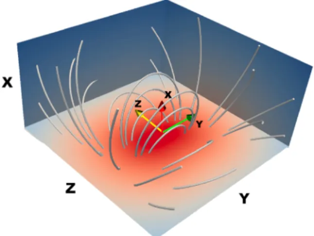
Figure 1. Typical simulation setup to study lunar magnetic anomalies
with iPi3D. The dipole center is situated on the X axis, just below the lunar surface (YZ plane). The dipole vector points along the Y axis. No interplanetary magnetic field is present in the shown setup. This cartoon, hence, shows the unperturbed dipole field.
Brackbill and Forslund, 1982; Lapenta et al., 2006] implemented in the code is
designed especially to overcome numer-ical constraints conventional explicit particle-in-cell codes suffer from, hence providing the ideal framework for mul-tiscale LMA simulations under various plasma conditions. Two extra func-tionalities are needed on top of the standard code: the possibility to have an external field superimposed on the background interplanetary magnetic field (IMF), representing the anomaly, and electromagnetic open boundary condi-tions (BCs) providing a uniform drifting Maxwellian plasma through the compu-tational box (See also Deca et al. [2013], for an implementation of the latter for electrostatic problems). The iPic3D code is publicly available on GitHub (https:// github.com/CmPA/iPic3D).
2.1. Implementation of the LMA Field
Typically, the LMA field structure is highly nondipolar [Mitchell et al., 2008], and a challenge on its own to model. Kurata et al. [2005], however, have proven that a combination of magnetic dipoles holds a good approx-imation in some cases. Following their strategy, the original implicit algorithm is modified to accommodate an external dipole magnetic field component B′, superimposed on the self-consistent (internal) magnetic
field B: B′(r) = 𝜇0 4𝜋 (3(m⋅ (r − r 0))(r − r0) (r − r0)5 − m (r − r0)3 ) ,
with the source located at r0and m the dipole moment (in Am2). Considering Cartesian coordinates, the plane YZ is chosen parallel to the lunar surface and the X direction is parallel to the unperturbed solar wind flow. The
dipole source location, r0, is embedded in the lunar regolith, and the configuration is illustrated in Figure 1. The external magnetic field B′is introduced in both the particle mover and the field solver, modeling in this
way both the influence of B′on the particles and the accompanied plasma response.
2.2. Open Boundary Conditions
Universal open boundary conditions (BCs) for particle-in-cell (PIC) simulations satisfying any arbitrary phys-ical problem are unfortunately a utopia, as proven by previous intense research in applications concerning, e.g., dipole-solar wind interaction problems [Buneman et al., 1992, 1993] or magnetic reconnection studies [Daughton et al., 2006; Divin et al., 2007; Klimas et al., 2008].
The iPic3D code, then, is no different. Extensive trial-and-error simulations converged to an approach similar to the implementation by Divin et al. [2007], producing a stable-flowing plasma when the solar wind speed is at least as fast as the thermal speed of the slowest plasma species in the simulation (not satisfying this condition leads to a significantly nonzero net charge in the box due to the mesosonic nature of the simulated plasma). The uniform drifting Maxwellian plasma through the computational box, having a thermal spread
vth,s, with s the species, and a bulk (solar wind) flow velocity vsw, is created according to the outline below. The particle BCs are enforced in three steps:
1. Fresh particles are generated every time step in a buffer layer of six cells near all boundaries with a velocity
vsw+ vth,s, where the solar wind velocity, vsw, is a fixed quantity, whereas vth,sis the random thermal velocity
of the species s. The amount of generated particles matches the initial solar wind density.
2. All the particles in the computational box are moved using the particle mover algorithm including the external LMA field.
3. The escaping particles (outside of the computational box) are removed from the simulation. Note that deleted particles do not leave any charge at the boundaries [Divin et al., 2007; Klimas et al., 2008], unlike charge-deposit schemes [Buneman et al., 1992, 1993].
In addition, one of the boundaries (x = 0) acts as a perfect absorber and represents the lunar surface. No particles are generated in the buffer layer on that side of the computational box nor is the charge of the outgo-ing particles collected. Note that at this moment the model does not include secondary particle and surface charging effects. Kallio et al. [2012] claim that these electrostatic processes are only significant in the first few tens of meters above the surface, and hence the general LMA interaction mechanism will, to first approxima-tion, not be affected. Surface charging and secondary particle effects (photoelectron and secondary electron emission) is the subject of future work.
Second, the most stable evolution for the LMA problem, implemented in the present work, is obtained under “fixed” field BCs, that is, for the fields E and B fixed to the initial (t = 0) value at the boundary cells. At first, such BCs seem to be in contradiction with the exact solution of the Maxwell set of equations, however, 1. Such BCs do not seem to produce boundary artifacts or numerical energy imbalance over the whole
simulation run.
2. The quiet solar wind, bringing a constant interplanetary magnetic field B = BIMFand carrying no current,
occupies most of the computational domain. In contrast, at the lunar side of the box the dipole field is very strong compared to the field produced by the induced currents. Hence, setting the magnetic field BCs as
B = B(t = 0) is justified in almost all boundary cells. Note that any deviation from the solenoidal condition,
∇⋅ B = 0, is corrected by the projection method used in the Poisson solver.
3. The electric field is advanced over time using a constant electric field set at the boundaries:
E = E(t = 0) = −vsw× BIMF. Any deviation from ∇⋅E = 4𝜋𝜌 is corrected using the Poisson solver. In addition,
a seven-point smoothing (in 3-D) is applied to the electric field every time step to reduce numerical noise. No significant tangential currents are produced at the boundaries using this setup.
2.3. Normalization
The numerical stability of a computer code can be significantly improved when all physical quantities, typically having a wide range of magnitudes, are scaled (close) to order 1 [Higham, 2002]. The iPic3D code therefore uses normalized cgs units internally, setting the speed of light c = 1, the ion mass per charge m∕e = 1, and the ion inertial length di= 1. A convenient consequence of this normalization procedure is that one and the same
simulation setup can apply to various physical systems, as long as the ratios of the dimensionless variables are identical [Markidis, 2010].
Three-dimensional large-scale simulations with a realistic speed of light and electron mass are rather expen-sive, and therefore, also reduced values are adopted for these quantities. All the simulations reported in this paper adopt an ion-to-electron mass ratio of mi∕me= 256 in which miis the reference value of mass for fur-ther calculations, and a speed of light value c∕vsw≈ 59, still ensuring a mesosonic solar wind flow, vsw, in all cases discussed. Note that the latter scaling does not affect the presented research [Bret and Dieckmann, 2010].
3. Results
3.1. General Interaction
To describe the general interaction of a dipole model centered just below the lunar surface under plasma con-ditions such that only the electron population is magnetized, we adopt a mesosonic electron-ion isothermal solar wind plasma at 1 AU, as a reference, in a temperature and velocity regime close to typical quiet solar wind conditions.
For the reference simulation (hereafter Run A if not indicated otherwise), the following physical parameters are utilized [Kivelson and Russell, 1995]: the plasma density is set nsw= 3 cm−3, corresponding to an ion
iner-tial length di ∼130 km; the ion and electron temperatures are Tsw = Ti = Te = 35 eV, and the solar wind
velocity vsw = (−350, 0, 0) km s−1. Note that for ease of computation Tswis chosen slightly higher than is
typical at 1AU. Although this common choice in PIC studies makes shorter the gyroradii, we have ensured ourselves that the overall structure and evolution of the minimagnetosphere is not significantly affected [see, e.g., Deca et al., 2014]. The interplanetary magnetic field BIMF = (0, 3, 0) nT is chosen antiparallel to the
dipole field (parallel to the dipole vector), hence creating a curved line of zero field strength in the magnetic topology in the Z direction. The gyroradii in the free-stream solar wind are re= 1.4×10⁴m and ri= 2.5×10⁵m
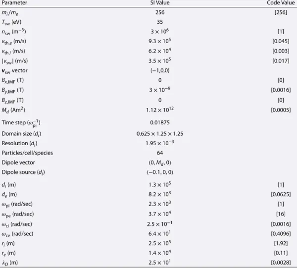
Table 1. Input Physical Parameters Used in the LMA Simulations and Reference Values in the Free-Streaming Solar Wind
for Run A in Both SI and Code Units (Between Square Brackets)
Parameter SI Value Code Value
mi∕me 256 [256] Tsw(eV) 35 nsw(m−3) 3 × 10⁶ [1] vth,e(m/s) 9.3 × 10⁵ [0.045] vth,i(m/s) 6.2 × 10⁴ [0.003] |vsw|(m/s) 3.5 × 10⁵ [0.017] vswvector (−1,0,0) Bx,IMF(T) 0 [0] By,IMF(T) 3 × 10⁻⁹ [0.0016] Bz,IMF(T) 0 [0] Md(Am2) 1.12 × 10¹² [0.0005] Time step (𝜔−1 pi) 0.01875 Domain size (di) 0.625×1.25×1.25 Resolution (di) 1.95 × 10⁻³ Particles/cell/species 64 Dipole vector (0, Md, 0) Dipole source (di) (−0.1, 0, 0) di(m) 1.3 × 10⁵ [1] de(m) 8.2 × 10³ [0.0625] 𝜔pi(rad/sec) 2.3 × 10³ [1] 𝜔pe(rad/sec) 3.7 × 10⁴ [16] 𝜔ci(rad/sec) 2.5 × 10⁻¹ [0.0016] 𝜔ce(rad/sec) 6.4 × 101 [0.4096] ri(m) 2.5 × 10⁵ [1.92] re(m) 1.4 × 10⁴ [0.11] 𝜆D(m) 2.5 × 101 [0.0028]
(at other locations within the simulation domain the radii can be read from Figure 7). Since the solar wind parameters can fluctuate significantly, we choose to adopt this rather high solar wind temperature to improve numerical stability. The dipole moment m = (0, Md, 0), where Md= 11.2 × 10¹²Am2, resembles the strongest
component of the two-dipole model for the Reiner Gamma magnetic anomaly region by Kurata et al. [2005]. The source is placed 13 km below the absorbing lunar surface. Note that, in general, the observed lunar mag-netic field topology is much more complicated and highly nondipolar [Hemingway and Garrick-Bethell, 2012]. To understand the complex interactions, studying a simple dipolar model is a necessary first step.
The size of the computational box measures (Lx, Ly, Lz) = (0.625, 1.25, 1.25) di, with the absorbing surface
located at x = 0 and the dipole placed at the point (−0.1, 0, 0). Initially low-resolution simulations were per-formed on a larger domain to ensure that the current size does not influence the plasma evolution in the box. The grid size is Nx × Ny × Nz = 320 × 640 × 640 with 64 particles per cell per species initially. Note that the electron scales are well resolved in our simulations: the electron skin depth de= 0.0625 di = 32 Δx,
with Δx the grid spacing. The time step is set relative to the ion plasma frequency: Δt = 0.01875 𝜔−1
pi
(= 0.00123 𝜏e = 4.8 × 10⁻⁶𝜏i), that is, thermal electrons pass only 0.4 Δx in 1 Δt. Note that the gyroperiods
are resolved well in the undisturbed solar wind, even close to the Moon where the surface magnetic field is strong. An overview of the physical and numerical simulation parameters is given in Table 1.
Figure 2 shows the 2-D electron and ion charge density profiles along the dipole axis (XY plane) at z = 0, after the simulation has reached quasi-steady state (after ∼8000 time cycles). Superimposed in black are magnetic field lines. The interplanetary magnetic field direction, BIMF, is opposite to the dipole magnetic field along the
Figure 2. Two-dimensional (top) electron and (bottom) ion charge density profiles, scaled to the initial density,nsw, and along the dipole axis (Y direction) atz = 0after the simulation has reached quasi-steady state. The solar wind is flowing perpendicular (in the−Xdirection) to the lunar surface. Superimposed in black are magnetic field lines.
line y = 0, z = 0, hence creating a zero-point in the total magnetic field configuration at 0.29 diabove the
surface, and thus a curve where B = 0 across the entire LMA in the Z direction.
As the solar wind impinges on the dipolar structure, perpendicular to the lunar surface, both the ion and electron populations are deflected toward the cusp regions, reflected upstream, or drift perpendicular to the magnetic field (see also section 3.2), and a density cavity is created that is surrounded by a higher density halo: a minimagnetosphere has formed. The halo region consists of solar wind particles which are temporarily packed against the dipole field close to the point where the magnetic pressure equals the solar wind plasma
Figure 3. Profiles along the direction parallel to the solar wind flow and through the center of the dipole. (top) The
density profiles, normalized to the initial densitynsw. The remaining panels hold the magnetic and kinetic pressure
Figure 4. Ion charge density profiles, scaled to the initial densitynsw, along three different planes: the (top left) XY plane and (bottom left) XZ plane through the dipole center, and the (right) YZ plane atx = 0.01 diabove the lunar surface. Superimposed in black are magnetic field lines. The red line indicates the 1-D cut made in Figure 6. The magenta stars indicate the sampling positions of Figures 8, 9, and 11.
pressure [Deca et al., 2014]. Note especially that the magnetic field line structure does not coincide with the charge density/magnetic pressure profile (Figure 3).
Under the present solar wind conditions, the halo has its highest point at 0.1 di(13 km) above the lunar regolith in the direction of the subsolar point. At this point the structure is about one electron skin depth (∼8 km) thick and has a maximum density approximately 1.6 times the solar wind value. A density gradient exists both in the halo, varying with position along the Y axis and toward the surface. Plasma is piled up most in the cusp regions (up to 3 times the initial density). The surface is best shielded between the cusps and the dipole center, meaning that both ions and electrons are more easily deflected with an increasing angle between the magnetic field and solar wind flow direction. On average, less than 10% of the electrons manage to reach the lunar surface within the minimagnetosphere density structure, in contrast to only 8% for the ions in the (small) best shielded regions and up to 60% toward the central region of the minimagnetosphere (Figure 4, right). Keep in mind that ion reflection from the surface is not incorporated in the numerical model. Given the scale size of the anomaly, only the electron population is magnetized, whereas the ions, due to their higher mass, should in principle only feel the dipole field much closer to the lunar surface before being scat-tered nonadiabatically (for reference, the electron and ion gyroradii at the halo location are re,halo≈ 10 km and
ri,halo ≈ 100 km, respectively). Ions thus easily penetrate the density halo farthest, creating a charge separa-tion between the two species. The latter results in the generasepara-tion of a large normal electric field, En, directed
along X toward the subsolar point (Figure 5). Note that the magnitude of 75mV/m is comparable to the values obtained by Jarvinen et al. [2014] (∼20mV/m), but since hybrid simulations do not resolve electrostatic effects, lower values in this model are to be expected. Large electric fields also exist in the cusp regions as a result of particles being trapped in the magnetic bottle created in between the cusps. Note as well the double-layer structure at x = 0.1 diabove the lunar surface, the exploration of which will be discussed elsewhere. Almost instantly after the start of the simulation, Enbecomes large enough to significantly deflect the thermal ion population at the halo altitude. The formation of the minimagnetosphere is therefore mainly an electrostatic effect and a direct consequence of charge separation in the halo region.
We do not observe a clear shock associated with the minimagnetosphere structure as the interaction region is much smaller than the gyroradii of the ions [Kallio et al., 2012] and plasma penetrates the halo at a too high speed for a stationary shock to exist [Shaikhislamov et al., 2013]. Making the analogy with Earth’s magneto-sphere [Harnett and Winglee, 2000; Kallio et al., 2012], however, one could refer to the higher-density barrier as an electrosheath rather than the magnetosheath, because the minimagnetosphere structure is formed due to electron dynamics [Deca et al., 2014].In connection with the latter comparison, no large scale deviations in
Figure 5. (top panel) Magnetic field magnitude and (bottom panels) electric field components in the XY plane (z = 0). Superimposed in black are magnetic field lines.
the magnetic field structure are observed with respect to the original Bdipole+ BIMFfield. The dipolar structure is compressed in the X direction and skewed in the −Z direction as the magnetized electrons also drag the magnetic structure with them when flowing along the electrosheath.
Turning our attention back to Figure 4, a much more complicated structure is observed in the XZ (perpendic-ular to the dipole axis) and YZ plane (at the lunar surface). The minimagnetosphere has an oval asymmetric density structure in the YZ plane close to the surface (Figure 4, right). At the lunar surface, the LMA measures approximately 65 km (0.5di) in Y and 80 km (0.6di) in the Z direction including the halo (0.2 di× 0.3 di
measur-ing only the density cavity). The halo (and consequently also the electrosheath) is not uniform on all edges and various substructures can be identified. The highest particle concentrations are found on the outside of the cusp regions where also the magnetic field direction is nearly perpendicular to the surface. Note from Figure 4 (bottom left), in comparison with the Figure 4 (top left), that the density profile along the halo in the
XZ plane is elongated toward the −Z direction.
Indeed, under the influence of the ∇B and E×B drift motions, the electrons packed against the halo are pushed in the −Z direction along the entire length of the electrosheath (see section 3.2.1 for more details). The much heavier ions, on the other hand, are deflected on all sides of the dipole structure by the normal electric field En,
and subsequently, an asymmetric density cavity/halo is created in response to the LMA field presence. Note that neither MHD nor hybrid simulations can fully model this configuration, because the process is initiated
Figure 6. (top) Total energy, (left column) electron, and (right column) ion velocity distributions along the profile
parallel to the solar wind flow and through the center of the dipole (see also Figure 4), normalized to code units. The distributions along the three axes are shown separately in the three subsequent panels.
by the electrons having highly non-Maxwellian velocity distributions near the minimagnetosphere structure (section 3.2.2).
3.2. Electron and Ion Dynamics
3.2.1. Particle Drifts and Halo Interaction
When the solar wind plasma approaches the electrosheath, the influence of the LMA and its associated elec-tric field, formed by charge separation and anchored in the minimagnetosphere halo boundary, increases with increasing magnitude of the fields toward the density structure. The electron population is significantly heated (Figure 6, top left) and accelerated in the −Z direction (Figure 6, bottom left), perpendicular to the dipole axis, by a combination of the magnetic (∇B+ curvature drift),
vB= mv 2 ⟂ 2eB3(B × ∇B) + mv2 ∥ eR2 cB2 (Rc× B), (1)
with Rcthe local radius of curvature and electric field drift (E × B + finite Larmor radius effect),
vE= (1 +1 4r 2 s∇ 2)E × B B2 (2)
[Baumjohann and Treumann, 1996] from the point downward where the electron kinetic pressure equals the magnetic field pressure at x = 0.23 di(Figure 3). The parameter rsis the local gyroradius of species s.
Evaluating the panels of Figure 7, the Z component of the electric field drift is prevalent by an order of mag-nitude for the lightest plasma species, thus formally predicting an overall motion of the electrons in the electrosheath toward the −Z direction. This is indeed what is observed in the simulations (e.g., Figure 6, bottom left). Note, since the ions are much heavier and moving with speed vswrather than vth,i perpendicu-lar to the magnetic field, the magnetic drift component dominates the electric field drift in this case. The ion population, however, is not magnetized and seems not to follow the motion dictated by the guiding-center theory and is deflected on all sides of the dipole structure by the normal electric field and the increasing mag-netic field pressure closer to the surface. A small deflection to the +Z direction is nevertheless observed close to the lunar surface (x = 0) in Figure 6 (bottom right) since the minimagnetosphere structure is skewed in the opposite direction as a result of the interaction with the plasma flow. The combination of the LMA and IMF field leads to areas within the simulation domain with vanishing magnetic fields, where the assumptions of the guiding-center theory are violated even for both particle species, i.e., close to the zero-line. Finally, since
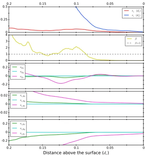
Figure 7. (top) Gyroradii of the two plasma species, plasma𝛽(𝛽 = 10in the free-stream solar wind plasma for (second panel) Run A), (third panel) normalized electric, and magnetic (bottom panels for the electron, respectively, ion population) particle drift estimates from the guiding-center theory (see equations (1) and (2)). The contribution of the finite Larmor radius effect (second order inrs, the respective gyroradii) is indistinguishable for both species, and subsequently, we plot only one curve in the second panel. The profile is along theY = 0,Z = 0line.
both the curvature drift (because of the relatively small v∥along the discussed cut) and the finite Larmor
radius effect (second order in rs) turn out to be negligible as compared to the ∇B and E × B components, we
will, from here onward, refer to the magnetic and electric field drifts as the ∇B and E × B drifts, respectively. Note that also Nishino et al. [2015] motivate the existence of double-loss-cone signatures above the Crisium Antipode anomaly in SELENE (Kaguya) observations via a ∇B drift mechanism. Similar indications are found in our simulations and are the subject of future work [see Deca, 2014, Figure 6.15].
The density along the solar wind flow and through the center of the dipole (Figure 3) starts rising at
0.15 di(≈19 km) above the surface, close to the point where the ion dynamic pressure equals the magnetic
pressure. The density peaks slightly closer at 0.1 di(≲13 km). In between those points a part of the ion kinetic
pressure is converted into thermal pressure causing the incoming ion flow to slow down by 50% of its original speed (Figure 6, second panel, right column). Most of the incident ions, however, penetrate the electrosheath and the halo region. The least energetic part of the ion population interacts with the halo causing ∼5% of the total incident plasma to be reflected back upstream, a number quantitatively consistent with observations by, e.g., Saito et al. [2012] (be it on the lower side of the observed range due to our idealized horizontal dipole field, see also section 4), and simulations, e.g., Kallio et al. [2012]. Within the electrosheath the solar wind ions are slowed down.
In this setup, the solar wind magnetic field direction, BIMF, is opposite to the dipole magnetic field along the line (y = 0, z = 0), creating a zero point in the total magnetic field configuration at 0.29 diabove the surface,
and by extension a line of magnetic nulls across the entire LMA structure in the Z direction. Notably, we do not observe any particle flows associated with magnetic reconnection, indicating that the minimagnetosphere
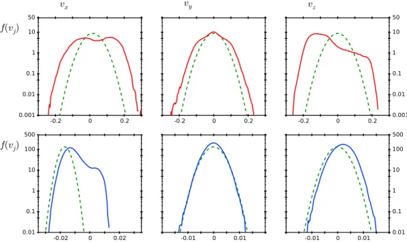
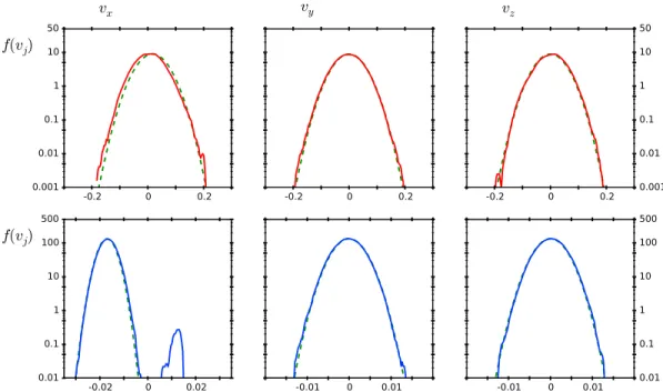
Figure 8. Ion (blue) and electron (red) particle distribution functionsf (vj)along the three axesj = x, y, z, respectively, sampled at 0.45diabove the lunar surface and directly upstream of the dipole source. For reference, a Maxwellian distribution with temperatureTswand drift velocityvsw, the reference values for the initial solar wind plasma (Table 2),
is displayed in dashed green as well.
electrosheath currents cannot shield off the dipole field completely, either because of the absorbing surface or the strongly nonadiabatic behavior of the ions [Shaikhislamov et al., 2013]. Increasing the magnetic dipole moment, however, can move the neutral line close enough to the density halo to produce favorable condi-tions for electron acceleration by the solar wind electric field, bringing more resemblance to a conventional large-scale (Earth) magnetosphere.
3.2.2. Particle Distribution Functions
After having presented the macroscopic structure of the minimagnetosphere and the general behavior of the plasma in the LMA field, we now shift our focus to the particle distribution functions on a few specific locations in the computational domain.
In Figure 8, the electron and ion particle distributions of vx, vyand vzare displayed just below the inflow bound-ary of the simulation box at 0.45diabove the lunar surface and directly upstream of the dipole source. This area
represents nearly the free-stream solar wind plasma, except for a reflected ion component seen in f (vx). The
1-D distribution functions f (vj) are constructed by grouping the vjvelocities into 200 uniform velocity bins in
the interval [vj,sw− 6vthj,s; vj,sw+ 6vthj,s] with j the direction and s the species, and using all particles per species available in an 8 × 8 × 8-cell cubic domain (0.016 di× 0.016 di× 0.016 di) with center (x, y, z) = (0.45, 0, 0) di.
In this chosen setup and for this particular position, the Y direction is considered parallel to the magnetic field, whereas the X and Z directions are perpendicular to B. Note that the green dashed line in Figure 8 is not a fit, but rather an upstream reference Maxwellian distribution with temperature Tswand drift velocity vsw, the reference values for the initial solar wind plasma (Table 2). Both the electron and ion distributions show, along the three directions, an almost perfect fit, as expected. Slight deviations are possibly due to the weak dipole field in combination with the IMF present at this location and a combination of small-scale numerical deviations in the initialization of the particle distributions. Note, the excellent agreement in Figure 8 does not only serve as a reference for later discussions but also proves that the open boundary conditions described in section 2.2 work correctly and produce the desired drifting Maxwellian plasma.
In addition to the drifting solar wind plasma, a second component in f (vx,i) is observed corresponding to parti-cles traveling upstream with an average speed of 0.012 (in code units), slightly slower than the incoming solar wind speed vsw = −0.017. The amount of back-streaming ions at this altitude accounts for only 0.5–1%
of the total ion population and finds its origin in the interaction of the solar wind with the minimagneto-sphere. A reflected component is present along the entire inflow plane as well as at the side boundaries of the
Table 2. Input Physical Parameters Used in the LMA Simulationsa Run A B C D E F G H I mi∕me 256 Tsw(eV) 35 nsw(m−3) 3 × 10⁶ [1] vth,e(m/s) 9.3 × 10⁵ [0.045] vth,i(m/s) 6.2 × 10⁴ [0.003] |vsw|(m/s) 3.5 × 10⁵ [0.017] 0.005 0.034 0.017 0.017 ̂vsw (−1,0,0) (−1,0,0) (−1,0,0) (−1,0,1) (−1,1,0) Bx,IMF(T) 0 [0] 0 0.00113 −0.0016 0 By,IMF(T) 6 × 10⁻⁹ [0.0016] −0.0016 0.00113 0 0.0032 Bz,IMF(T) 0 [0] 0 0 0 0 |BIMF| 6 × 10⁻⁹ [0.0016] 0.0016 0.0016 0.0016 0.0032 Md(Am2) 1.12 × 10¹² [0.0005]
aAs a reference, the values for Run A are displayed in both SI and code units (between square brackets) where
applicable. For all other simulations only code units are shown. Only the numbers changed with respect to Run A are repeated.
simulation domain at an angle consistent with the direction to the LMA origin. The minimagnetosphere thus reflects ions in all possible directions away from its density structure. The strongest reflected component is observed directly above the LMA. Lower resolution simulations (not included here) indicate a detectable reflected ion population up to 0.5 riupstream (125 km above the lunar surface).
Moving closer to the halo, the back-streaming ion component enlarges. At 0.15 diabove the surface (0.05 di
above the halo center), the population of reflected ions is approximately 6% of the incident solar wind density (Figure 9), the average particle streaming up at a speed vx= 0.01. The distribution is non-Maxwellian. Looking
from high to low reflection velocities, the profile rises steep at vx= 0.014 but has a more elongated tail toward zero, indicating a cutoff value for the reflected ion speed. Assuming that incident particles with high energy
Figure 9. Ion (blue) and electron (red) particle distribution functionsf (vj)along the three axesj = x, y, z, respectively, sampled at 0.15diabove the lunar surface (0.05 diabove the halo center) and directly upstream of the dipole source. For reference, a Maxwellian distribution with temperatureTswand drift velocityvsw, the reference values for the initial solar wind plasma (Table 2), is displayed in dashed green as well.
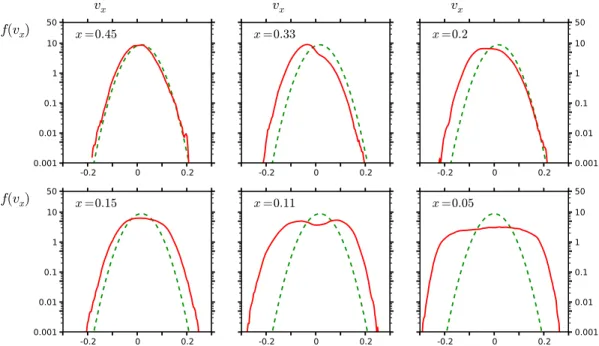
Figure 10. Electron particle distribution functions along the X axis (red), sampled at six locations above the lunar
surface and directly upstream of the dipole source, as indicated in the top left corner of each panel (in code units). For reference, a Maxwellian distribution with temperatureTswand drift velocityvsw, the reference values for the initial solar wind plasma (Table 2), is displayed in dashed green as well.
are also reflected with higher velocities, one can conclude that particles traveling at higher velocities than the cutoff value will simply pass through the halo, unable to be stopped by the normal electric field above in the halo. The elongated tail of the distribution disappears farther upstream. The more energetic the ion on reflection, the farther upstream it will travel [Savoini et al., 2013]. As mentioned before, the incoming solar wind ion population is slowed down by the strong normal electric field component. The original Maxwellian velocity distribution, however, is preserved in all three directions and the plasma is decelerated as a whole for
−0.03 ≤ x ≤ −0.01. Although not shown, at x = 0.1 di, inside the pileup region, both components of f (vx,i)
have become indistinguishable (vx= −0.01) and f(vz,i) is shifted by vz= 0.003 at this altitude. Note that f(vy,i) is seemingly unaffected by the various interactions at play close to the minimagnetosphere.
Focusing on the electron distribution functions then, no clear deflections from the initial Maxwellian are observed at and higher than x = 0.4 di(x = 6.4 de) above the lunar surface (Figure 10, top left). Below this
altitude, a suprathermal wing becomes noticeable in the upstream (−X) direction of the distribution func-tion along vx(Figure 10, top middle). Note, the sampling box is still well above the zero point in the field at
x = 0.29 di. The asymmetric profile evolves into a flat-top distribution at x = 0.2 di(0.1 diabove the halo,
Figure 10, top right) when the slowest electrons become influenced by the E × B drift mechanism. Note that at this point we have surpassed the zero point in the magnetic field topology as well without observing the electron distributions typically associated with a reconnection region [see, e.g., Asano et al., 2008]. In Figure 10 (bottom middle), the distribution at 0.01 diabove the halo (0.11 diabove the surface) is shown. A clear bimodal
(double-bump) profile prevails with mean velocities vx,1 = 0.1 and vx,2 = −0.06, a signature of a loss-cone distribution, indicating that the electrons most likely undergo mirror reflection (Fermi acceleration) at the density halo similar to processes observed in the Earth’s foreshock region [Leubner and Vörös, 2012; Savoini
and Lembège, 2001].
A symmetric suprathermal distribution is observed in the component parallel to the magnetic field (Figure 11, top middle). Two clear components in the f (vz,e) are present here as well (Figure 11, top left); an isotropic flat-top distribution with a superimposed significantly accelerated beam with average speed vz = −0.017.
Electrons are thus scattered and accelerated in the −Z direction. Moving inside the halo, both perpendicular components (X and Z) evolve into a flat-top distribution, while along the parallel direction the electrons are further thermalized.
Figure 11. Ion (blue) and electron (red) particle distribution functionsf (vj)along the three axesj = x, y, z, respectively, sampled at 0.11diabove the lunar surface (0.01 diabove the halo center) and directly upstream of the dipole source. For reference, a Maxwellian distribution with temperatureTswand drift velocityvsw, the reference values for the initial solar wind plasma (Table 2), is displayed in dashed green as well.
4. Discussion: Impact of the Plasma Environment
As many characteristics of the solar wind-LMA interaction discussed above are highly dependent on the fea-tures of the lunar and upstream plasma environment, it is interesting to detail how the minimagnetosphere structure and its shielding efficiency changes with changing solar wind conditions. We focus in this discus-sion on the influence of both the IMF and solar wind direction/strength on the macroscopic structure of the minimagnetosphere in comparison with the above discussion. By changing only one parameter at the time in the various simulations, the impact of every factor is most easily evaluated. An overview of the parameter set for the different runs is presented in Table 2. Note, in the following discussion only the most relevant quan-tities are included in the figures. The reader may safely assume that, unless otherwise mentioned, quanquan-tities not shown behave similarly to the reference run A discussed in section 3.
4.1. The Interplanetary Magnetic Field 4.1.1. Varying the IMF Direction
Keeping the magnitude of the IMF constant, we vary its direction only and consider three more cases (runs B–D in Table 2). Figure 12 shows the main characteristics of the density and magnetic field structure along the dipole axis and perpendicular to the lunar surface at x = 0.01 di.
At first sight, comparing to run A discussed above, the IMF direction has little impact on the overall density structure of the minimagnetosphere, although the magnetic field structure outside the density halo is very different from one case to another. This is not entirely surprising, as the dipole field at the halo is an order of magnitude larger than|BIMF|. Run B produces a more round structure compared to Run A, whereas for Runs C
and D the shielding region is skewed because the IMF interacts with the dipole field with an asymmetric angle. Note that in the bottom panel for Run B in Figure 12 two bands/spots of higher density are present within the outer halo (most pronounced for positive Z values). These correspond to particles initially penetrating the halo before being pushed outward.
The halo stabilizes in all four cases at x = 0.1 diabove the lunar surface. The width of the pileup region is similar as well for all but Run B, where an IMF antiparallel to the dipole vector, hence not producing a line of zero magnetic field above the LMA structure, results in a much wider halo area. Without the IMF opposing the dipole magnetic field, the minimagnetosphere magnetic field compresses less and a more gentle tran-sition from the solar wind to the LMA influence region causes a 25% weaker normal electric field above the
Figure 12. Electron charge density profiles, scaled to the initial densitynsw, along two different planes: the (top) XY plane and (bottom) YZ plane atx = 0.01 di
above the lunar surface for Runs A–D (see also Table 2). Superimposed in black are magnetic field lines.
halo. Subsequently, both the ions and the electron population, the latter due to a slower E × B drift motion component, are allowed to penetrate deeper into the halo, affecting also the number of back-streaming ions. In Run B, at 0.05 diabove the halo (x = 0.15 di) there are significantly less reflected particles detected in the
electrosheath as compared to Run A. Second, the average back-streaming speed of the latter is found 20% lower. Only the least energetic ions from the incoming distribution are reflected, hence reducing the average back-streaming speed relative to the incoming solar wind ions. For reference, we find that on average 6.1%, 4.9%, 5.%, and 4.8% of the incoming ion plasma are reflected by the normal electric field above the halo for Runs A–D, respectively. These numbers are obtained at steady state by counting the number of ions with an upward (positive vx) component with respect to the downward (negative vx) moving ion population at 0.05 di
above the halo (x = 0.15 di). 4.1.2. Varying the IMF Magnitude
Taking Run A as a reference, lowering the IMF magnitude leads to a curve of zero magnetic field farther away from the lunar surface and a decreased impact on the magnetic structure of the minimagnetosphere (not shown). Within the influence region of the LMA, the system behaves more and more similar to Run B with decreasing IMF.
Increasing the IMF magnitude with a factor of 2 (Run E in Table 2, Figure 13), on the other hand, brings the center of the density halo 0.01 difarther downstream and makes the overall area of the minimagnetosphere shrink by 35%, measured at the surface. The magnetic field zero-point along the profile y = 0, z = 0 shifts from 0.29 dito 0.20 diabove the lunar surface. The consequence is that now the electric field and the
elec-tron current profile in the electrosheath become spatially connected with the B = 0 curve in the magnetic field. Second, above the dipole source the angle of the magnetic field vector to the surface normal is larger as compared to Run A, i.e., the nose of the LMA magnetic structure becomes more sharp. The latter improves the shielding efficiency of the minimagnetosphere for both ions and electrons. Although only 4.2% of the ion dis-tribution is reflected, a larger component of the population is deflected/scattered toward the cusps and outer edges of the density structure, resulting in less that 40% of the incoming ions reaching the surface within the density halo. More than 98% of the electron population is shielded away by the minimagnetosphere. In particular, the center region of the LMA receives much less solar wind particles. Remind that our simulation model does not (yet) include charged dust, photoelectron and secondary electron, and possibly collisions, which might play a role in supporting charge balance in this region [Howes et al., 2015]. In Figure 13, the elec-tron charge density profile is illustrated with the superimposed magnetic field lines in the XY plane. Note especially the very weak higher-density pattern connecting the cusp regions with the zero point
Figure 13. Electron charge density profile, scaled to the initial densitynsw, along the XY plane for Run E. The very weak higher-density pattern connecting the cusp regions with the zero point is indicated with a blue ellipse. Superimposed in black are magnetic field lines.
(indicated with a blue ellipse), which is observed over the entire length of the halo in the Z direction. No clear signature is found in the electron currents nor the distribution functions, however, connecting the mag-netic field topology with this particular phenomenon in the charge density profile. This observation deserves further and more detailed investigation.
4.2. The Solar Wind Plasma
4.2.1. Varying the Solar Wind Speed
To investigate the effect of the solar wind speed on the minimagnetosphere interaction, we take once more Run A as a reference and compare with the results of a simulation initialized with a slower (vsw = 0.005 =
103km/s, Run F) and faster (vsw = 0.034 = 700 km/s, Run G) drifting solar wind plasma (see Table 2 for an overview of the complete parameter set of the simulations).
The faster the solar wind impinges onto the LMA field, the more the minimagnetosphere is compressed. Eval-uating the profile perpendicular to the surface and through the dipole source (Figure 14), we find the zero point in the field at 0.33 di, 0.29 di, and 0.23 diabove the lunar surface for runs F, A, and G respectively. Other
than the obvious, some interesting features can be noted. The solar wind speed initialized in Run F is only marginally higher than the ion thermal speed, and a strong enough normal electric field does not emerge to form a density halo. The density of both species toward the surface (Figure 15), however, decreases steadily as the particles are scattered toward the magnetic cusps by the magnetic pressure, rather than deflected into the Z-direction by the E × B drift. The shielding efficiency of the structure is reduced but still significant as less than 1% of the electrons reaches the center of the LMA, and the best shielded regions still receive only 20% of the incoming solar wind ions. No back-streaming ion population is observed for Run F.
Figure 14. Density profiles along the direction parallel to the solar wind flow and through the center of the dipole for
Figure 15. Ion charge density profiles, scaled to the initial densitynsw, along two different planes: the (top) XY plane and (bottom) YZ plane atx = 0.01 diabove the lunar surface for Runs F, A, and G (see also Table 2). Superimposed in black are magnetic field lines.
In the XY plane, the ion charge density profile of Run G shows similar features as the reference Run A; a clear density pileup is observed at 0.07 diabove the lunar surface as well as higher density cusp regions
and a shielded area protecting the surface from the impinging plasma. The electron charge density profile (Figure 14, top), on the other hand, does not develop a halo directly above the dipole source, but rather a gen-tle increase followed by a sudden drop prevails where the ion pileup region is found. Due to the high solar wind speed, a stronger normal electric field is formed in response to the charge separation caused by a faster flowing ion population penetrating deeper into the dipole field. This results in a much stronger E × B drift component deflecting most of the electron population before a pileup region can be formed. The ion den-sity, on the other hand, loses its typical asymmetric shape and is almost circularly reflected around the dipole center by the increasing magnetic pressure. More than 80% of the incoming ion plasma still reaches the central LMA undisturbed.
To conclude this subsection, we point the reader to energetic neutral atom observations by Chandrayaan-1. Analyzing the influence of the solar wind dynamic pressure on the shielding efficiency at the Gerasimovich anomaly, Vorburger et al. [2012] concur on a higher shielding efficiency under lower solar wind dynamic pres-sure, in agreement with our simulation results. Additionally, Vorburger et al. [2012] admit that estimating the shielding efficiency of magnetic anomalies is more complex than the Gerasimovich case, as for many observed anomalies no correlation could be proven. Indeed, also from a simulation point of view, adopting an idealized dipole model is not straightforward under changing solar wind conditions.
4.2.2. Varying the Solar Wind Direction
The impact of the solar wind direction on the minimagnetosphere structure is illustrated in Figure 16 with two examples representing a possible situation closer to the lunar terminator: Run H, in which the solar wind flows at a 45∘angle with the absorbing surface and parallel to the dipole axis (vsw= (−0.012, 0, 0.012)), and Run I, having vswat the same angle to the surface, but perpendicular to the situation initialized in Run H
Figure 16. Ion charge density profiles, scaled to the initial densitynsw, along the YZ plane atx = 0.01 diabove the lunar surface for (left) Run H and (right) I.
Comparing once more with the reference Run A, which has an identical solar wind velocity in magnitude but drifts perpendicular to the surface, all typical features in the density profile of the minimagnetosphere can be recognized: the density halo and depletion region, and a density increase to what should correspond to the magnetic cusp regions. For Run H, these higher density areas are indeed similar to Run A. With the solar wind plasma now arriving at an angle to the surface and thus also to the direction of the magnetic moment, the minimagnetosphere structure is merely pushed into a more oblique direction. This results in more elon-gated magnetic cusp regions and accordingly a density halo which is skewed in the same direction (Figure 16, left). The higher density regions on the surface connected to the magnetic cusps are larger and also shielding of the lunar regolith in between has improved considerably as the plasma particles, especially the ion pop-ulation, need to be only diverted rather than reflected away. The center region of the minimagnetosphere is completely off limit for the electrons, while less than 5% of the ions manages to reach the surface.
For Run I (Figure 16), on the other hand, the magnetic structure arising is more complicated (as compared to the reference run A) as the dipole field bends from its original dipole orientation in accordance with the flow direction. Most plasma arriving at the upstream end of the LMA is accumulated at the magnetic (upstream) cusp, whereas no significantly higher-density region is observed at the downstream cusp. Very little plasma reaches the latter position, and the field lines which should build the downstream magnetic cusp emerge from the surface entirely within the shielded region of the minimagnetosphere. A more pronounced pileup region, comparable to the upstream magnetic cusp, is only present at the −Y side of the LMA, formed by particles deflected to the surface by the changing magnetic pressure profile over space. The +Y side of the structure is characterized by a wider area of less elevated charge density because the E × B drift, mostly prevalent at the upstream minimagnetosphere boundary, causes the plasma to deflect and scatter over the downstream side of the LMA. Note once more that also in this case the surface within the halo is much better shielded as compared to a solar wind direction perpendicular to the surface.
5. Conclusions
We have presented in detail three-dimensional full-kinetic and electromagnetic simulations of the solar wind interaction with lunar crustal magnetic anomalies (LMAs). Using iPic3D in its fully electromagnetic version, we confirmed that, at least under typical quiet solar wind conditions, LMAs may indeed be strong enough to stand off the solar wind from directly impacting the lunar surface forming a so-called “minimagnetosphere,” as suggested by spacecraft observations and theory.
We implemented the code structure needed to incorporate the LMA field and developed electromagnetic open boundary conditions. The latter is crucial to produce a drifting Maxwellian plasma through the compu-tational box, indispensable for solar wind-body interaction studies. Using a dipole model centered just below an absorbing surface representing the lunar regolith, we described the interaction of an idealized LMA under plasma conditions such that only the electron population is magnetized. Studying in detail the field structure
and particle dynamics, we showed that the LMA configuration is driven by electron motion, because its scale size is small with respect to the gyroradius of the solar wind ions.
When the kinetic pressure meets the magnetic pressure of the magnetic dipole, charge separation due to the mass difference between the plasma species sets up a normal electric field along the −X direction at the subsolar point. The latter is responsible for the population of back-streaming ions identified at the upwind simulation boundary, the deflection of magnetized electrons via the E × B drift motion, and the subsequent formation of a halo region of elevated density around the dipole source. All three effects together made that inside the density barrier the lunar regolith is well shielded from the electron population (less than 5% reached the surface). The shielding properties of the minimagnetosphere for the ion plasma were found to be more coupled to the solar wind plasma parameters as compared to the much lighter electrons. The shield-ing efficiency improved substantially with decreasshield-ing solar wind speed and angle of the solar wind direction to the surface. The IMF had, in comparison, only a weak effect on the overall structure and evolution of the LMA system.
The simulation results are ideally suited to be compared with field or particle observations from spacecraft such as Kaguya (SELENE), Lunar Prospector, or ARTEMIS, especially in terms of its impact on basic science, instrument disturbances, and lunar exploration in general. Note finally, that understanding LMAs and min-imagnetospheres is not only important for lunar science. Also, Mars has no longer a global magnetic field but only crustal magnetization [Acuna et al., 1999]. In this respect NASA’s MAVEN (Mars Atmosphere and Volatile EvolutioN) mission [Jakosky, 2009], which arrived at the Red Planet late September 2014, is of particu-lar importance. MAVEN is the first spacecraft exploring the Martian upper atmosphere, including its magnetic anomalies. More down to Earth, the construction and shielding effectiveness of artificial minimagnetospheres are explored extensively for future human space flight [Bamford et al., 2014]. The result of the latter will, hope-fully, provide the framework for spacecraft engineers to converge to realistic estimates of the risks, needed resources and effectiveness of radiation protection for long-duration human space missions.
References
Acuna, M. H., et al. (1999), Global distribution of crustal magnetization discovered by the Mars global surveyor MAG/ER experiment, Science,
284, 790–793, doi:10.1126/science.284.5415.790.
Asano, Y., et al. (2008), Electron flat-top distributions around the magnetic reconnection region, J. Geophys. Res., 113, A01207, doi:10.1029/2007JA012461.
Ashida, Y., H. Usui, I. Shinohara, M. Nakamura, I. Funaki, Y. Miyake, and H. Yamakawa (2014), Full kinetic simulations of plasma flow interactions with meso- and microscale magnetic dipoles, Phys. Plasmas, 21(12), 122903, doi:10.1063/1.4904303.
Bamford, R., B. Kellett, J. Bradford, T. N. Todd, R. Stafford-Allen, E. P. Alves, L. Silva, C. Collingwood, I. A. Crawford, and R. Bingham (2014), An exploration of the effectiveness of artificial mini-magnetospheres as a potential solar storm shelter for long term human space missions,
ArXiv e-prints.
Bamford, R. A., B. Kellett, W. J. Bradford, C. Norberg, A. Thornton, K. J. Gibson, I. A. Crawford, L. Silva, L. Gargaté, and R. Bingham (2012), Minimagnetospheres above the lunar surface and the formation of lunar swirls, Phys. Rev. Lett., 109(8), 81101,
doi:10.1103/PhysRevLett.109.081101.
Baumjohann, W., and R. A. Treumann (1996), Basic Space Plasma Physics, Imperial College Press, London, U. K.
Belmont, G., R. Grappin, F. Mottez, F. Pantellini, and G. Pelletier (2013), The magnetized plasmas, pp. 77–104, Wiley–VCH Verlag GmbH and Co. KGaA, Los Angeles, Calif., doi:10.1002/9783527656226.ch3.
Brackbill, J. U., and D. W. Forslund (1982), An implicit method for electromagnetic plasma simulation in two dimensions, J. Comput. Phys., 46, 271–308, doi:10.1016/0021-9991(82)90016-X.
Bret, A., and M. E. Dieckmann (2010), How large can the electron to proton mass ratio be in particle-in-cell simulations of unstable systems?,
Phys. Plasmas, 17(3), 32109, doi:10.1063/1.3357336.
Buneman, O., T. Neubert, and K.-I. Nishikawa (1992), Solar wind-magnetosphere interaction as simulated by a 3-D EM particle code, IEEE
Trans. Plasma Sci., 20, 810–816, doi:10.1109/27.199533.
Buneman, O., K.-I. Nishikawa, and T. Neubert (1993), Solar wind-magnetosphere interaction as simulated by a 3-D, EM particle code, in Plasma Physics and Controlled Nuclear Fusion (ITC-4), edited by H. T. D. Guyenne and J. J. Hunt, pp. 285–288, ESA.
Daughton, W., J. Scudder, and H. Karimabadi (2006), Fully kinetic simulations of undriven magnetic reconnection with open boundary conditions, Phys. Plasmas, 13(7), 72101, doi:10.1063/1.2218817.
Deca, J. (2014), Multi-scale kinetic simulations with iPic3D: From spacecraft charging analysis to the solar wind interaction with lunar magnetic anomalies, PhD thesis, KULeuven/Arenberg Doctoral School, Leuven.
Deca, J., G. Lapenta, R. Marchand, and S. Markidis (2013), Spacecraft charging analysis with the implicit particle-in-cell code iPic3D, Phys.
Plasmas, 20(10), 102902, doi:10.1063/1.4826951.
Deca, J., A. Divin, G. Lapenta, B. Lembège, S. Markidis, and M. Horányi (2014), Electromagnetic particle-in-cell simulations of the solar wind interaction with lunar magnetic anomalies, Phys. Rev. Lett., 112(15), 151102, doi:10.1103/PhysRevLett.112.151102.
Divin, A. V., M. I. Sitnov, M. Swisdak, and J. F. Drake (2007), Reconnection onset in the magnetotail: Particle simulations with open boundary conditions, Geophys. Res. Lett., 34, L09109, doi:10.1029/2007GL029292.
Dolginov, S. S., and N. V. Pushkov (1960), Magnetic field of the outer corpuscular region, Int. Cosmic Ray Conf., 3, 30–31.
Dyal, P., C. W. Parkin, and C. P. Sonett (1970), Apollo 12 magnetometer: Measurement of a steady magnetic field on the surface of the Moon,
Science, 169, 762–764, doi:10.1126/science.169.3947.762.
Acknowledgments
This research has received funding from the European Commission’s FP7 Program under the grant agree-ment EHEROES (project 284461, www.eheroes.eu). The simulations were conducted on the computational resources provided by the PRACE Tier-0 project 2011050747 (Curie supercomputer) and 2013091928 (SuperMUC supercomputer). J.D. has received support through the HPC-Europa2 visitor program (project HPC08SSG85) and the KuLeuven Junior Mobility Program Special Research Fund. Test simulations were performed by A.D. on resources provided by SNIC at PDC Centre for High Performance Computing (PDC-HPC), grants m.2014-8-38 and m.2014-1-176. This work was also supported in part by NASA’s Solar System Exploration Research Virtual Institute (SSSERVI): Institute for Modeling Plasmas, Atmo-sphere, and Cosmic Dust (IMPACT). Access to the raw data may be provided upon motivated request to J.D.
Yuming Wang thanks two anonymous reviewers for their assistance in evaluating this paper.


![Table 2. Input Physical Parameters Used in the LMA Simulations a Run A B C D E F G H I m i ∕m e 256 T sw (eV) 35 n sw (m −3 ) 3 × 10 6 [1] v th,e (m/s) 9](https://thumb-eu.123doks.com/thumbv2/123doknet/14773146.592361/13.918.260.863.150.416/table-input-physical-parameters-used-lma-simulations-run.webp)