First-principles modeling of geomagnetically induced electromagnetic fields and currents from upstream solar wind to the surface of the Earth

HAL Id: hal-00318307

https://hal.archives-ouvertes.fr/hal-00318307

Submitted on 8 May 2007

HAL is a multi-disciplinary open access

archive for the deposit and dissemination of

sci-entific research documents, whether they are

pub-lished or not. The documents may come from

teaching and research institutions in France or

abroad, or from public or private research centers.

L’archive ouverte pluridisciplinaire HAL, est

destinée au dépôt et à la diffusion de documents

scientifiques de niveau recherche, publiés ou non,

émanant des établissements d’enseignement et de

recherche français ou étrangers, des laboratoires

publics ou privés.

electromagnetic fields and currents from upstream solar

wind to the surface of the Earth

A. Pulkkinen, M. Hesse, M. Kuznetsova, L. Rastätter

To cite this version:

A. Pulkkinen, M. Hesse, M. Kuznetsova, L. Rastätter. First-principles modeling of geomagnetically

induced electromagnetic fields and currents from upstream solar wind to the surface of the Earth.

Annales Geophysicae, European Geosciences Union, 2007, 25 (4), pp.881-893. �hal-00318307�

www.ann-geophys.net/25/881/2007/ © European Geosciences Union 2007

Annales

Geophysicae

First-principles modeling of geomagnetically induced

electromagnetic fields and currents from upstream solar wind to the

surface of the Earth

A. Pulkkinen1,2, M. Hesse2, M. Kuznetsova2, and L. Rast¨atter2,3

1_{Goddard Earth Sciences and Technology Center, University of Maryland, Baltimore, MD, USA} 2_{NASA/GSFC, Greenbelt, Code 674, MD 20771, USA}

3_{Catholic University, Washington D.C., USA}

Received: 20 November 2006 – Revised: 5 April 2007 – Accepted: 13 April 2007 – Published: 8 May 2007

Abstract. Our capability to model the near-space physical

phenomena has gradually reached a level enabling module-based first-principles modeling of geomagnetically induced electromagnetic fields and currents from upstream solar wind to the surface of the Earth. As geomagnetically induced cur-rents (GIC) pose a real threat to the normal operation of long conductor systems on the ground, such as high-voltage power transmission systems, it is quite obvious that success in ac-curate predictive modeling of the phenomenon would open entirely new windows for operational space weather prod-ucts.

Here we introduce a process for obtaining geomagneti-cally induced electromagnetic fields and currents from the output of global magnetospheric MHD codes. We also present metrics that take into account both the complex na-ture of the signal and possible forecasting applications of the modeling process. The modeling process and the met-rics are presented with the help of an actual example space weather event of 24–29 October 2003. Analysis of the event demonstrates that, despite some significant shortcomings, some central features of the overall ionospheric current fluc-tuations associated with GIC can be captured by the model-ing process. More specifically, the basic spatiotemporal mor-phology of the modeled and “measured” GIC is quite simi-lar. Furthermore, the presented user-relevant utility metrics demonstrate that MHD-based modeling can outperform sim-ple GIC persistence models.

Keywords. Ionosphere (Auroral ionosphere; Modeling and

forecasting) – Space plasma physics (Numerical simulation studies)

Correspondence to: A. Pulkkinen

(antti.pulkkinen@gsfc.nasa.gov)

1 Introduction

Over the past few years there has been great progress in establishing extensive space weather frameworks having an ambitious goal of module-based modeling of the space weather phenomenon from the Solar surface to the planetary ionospheres (see T´oth et al., 2005, and references therein). Obviously, self-consistent modeling of physical phenomena in near-Earth space provides an unprecedented capability to gain new understanding about the Solar surface, corona, he-liosphere, magnetosphere and ionosphere systems behavior as a whole. However, although much of space weather is covered within the Solar surface and Earth’s ionosphere, the space weather phenomena do not end there; the processes ex-tend down to the surface and below the surface of the Earth in terms of geomagnetic induction driven by variations in the near-space current systems.

From the applications viewpoint, extending the space weather frameworks to include the geomagnetic induction component provides new tools for mitigating geomagneti-cally induced currents (GIC) flowing in long conductor sys-tems on the ground (e.g., Boteler et al., 1998; Molinski, 2002; Pirjola et al., 2004). Based on the sole impact of the famous March 1989 storm on the North American power transmis-sion system (e.g., Czech et al., 1992; Bolduc, 2002), it is safe to say that GIC is one of the most important space weather hazards and that need for science-based mitigation capabil-ities is real. However, the present mitigation capabilcapabil-ities are limited mostly to statistical estimates based on histori-cal data and to nowcasting of GIC levels (e.g., Pulkkinen et al., 2001b; Viljanen et al., 2006b; Boteler et al., 2006). It fol-lows that success in accurate modeling enabling forecasting discussed in this work would open a new avenue for science-based GIC mitigation with true potential for commercial applications. Obviously, such applications would give an

appealing additional societal justification for the work put into the large number of space physical models involved in the modeling chain.

Work presented here is by no means the first attempt to use information from the upstream solar wind to estimate the level of GIC fluctuations. Relatively successful empirical ef-forts have been made to reproduce some features of GIC, or proxies of GIC (Weigel et al., 2003; Wintoft, 2005). How-ever, although similar activities are underway at the Darth-mouth College1 and some properties of the time derivative of the ground magnetic field given by global magnetohydro-dynamic (MHD) modeling have been analyzed by Raeder et al. (2001b), the work at hand is the first reported attempt to carry out GIC modeling by using first-principles models. By first-principles modeling we refer here to the process of solv-ing the evolution equations of the system, or coupled systems as is done here, derived using elementary physical principles. This is in contrast to empirical modeling procedures where observations are used to derive the equations. Although em-pirical models have their important role in acquiring under-standing about the behavior of the system, a first-principles approach is the natural ultimate goal for the modeling of any physical system. Thus, although the well-known limitations of, for example, MHD modeling (these limitations will be discussed more in detail below) lower some of the expecta-tions for the accuracy of the final output of our interest, it is worthwhile to start moving toward this goal.

The work presented here comprises Phase 1 of the project dedicated to test the present capabilities of first-principles modeling of space weather from the ground and especially from the GIC viewpoint. More specifically, in the work at hand we will present the basic modeling process for obtain-ing the quantities of our interest from the output of the MHD codes. We will also explore metrics that take into account both the complex nature of the signal and possible forecast-ing applications of the modelforecast-ing process; the selected metrics will be one of the backbones of the future work. Although the modeling process and the metrics are introduced with the help of an actual example space weather event of 24– 29 October 2003, rigorous testing utilizing different model setups and framework components will be carried out later in Phase 2 of the project.

The structure of the paper is as follows. First, in Sect. 2 we will go through the various steps of the modeling pro-cess leading to induced electromagnetic fields on the ground. Once the induced electric field is known, GIC in individual technological systems can be easily computed. In Sect. 3, we will model the space weather event of 24–29 October 2003. The output, geomagnetically induced electromagnetic fields and currents, are then compared to the measured quantities and the performance of the modeling chain is evaluated qual-itatively. In Sect. 4, we explore the metrics appropriate for

1_{http://engineering.dartmouth.edu/}∼_{simon/research/GIC/index.}

html

quantifying the model performance especially from the GIC viewpoint. The model output of the example event is then evaluated using the selected metrics. Finally, in Sect. 5 we briefly summarize and discuss the findings of the study.

2 Modeling process

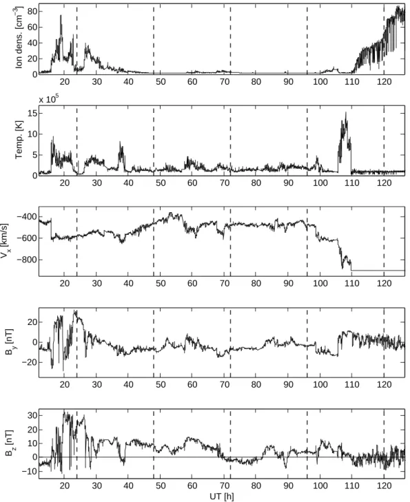
The core of the modeling process realized here is composed of the three-dimensional (3-D) global magnetospheric MHD code BATS-R-US (Powell et al., 1999) coupled to a two-dimensional electrostatic ionospheric inner boundary model (Ridley et al., 2004). The code was driven using convection delayed L1 solar wind plasma and magnetic field observa-tions for a period of 24 October 2006 11:28 UT–29 October 2006 06:28 UT (see Fig. 1). Without trying to make any more definite estimation for the errors here, it is noted that inaccu-racies in the solar wind propagation to the model boundary will inevitably lead to inaccuracies in the timing of the mod-eled field fluctuations (see, e.g., Bargatze et al., 2005, and references therein). This issue will be studied more in detail in the follow-up of this initial study. The run was carried out utilizing the facilities at the Community Coordinated Mod-eling Center (CCMC) operating at NASA Goddard Space Flight Center and the state of the system was recorded every 4 min, which dictated the temporal resolution of further mod-eling. Consequently, all data presented in this paper are aver-aged to a 4-min time resolution. On the ionospheric side, au-roral conductance model was used in the ionospheric poten-tial solver. We used a relatively sparse magnetospheric grid, the minimum cell width being 0.5 RE (Earth radii), which

resulted in about 300 000 global MHD model cells. The ob-jective in using such a poor resolution was to be able to carry out the run in a realistic operational setup; the same setup is used currently at CCMC for real-time runs of the BATS-R-US. These runs are made with three parallel nodes each of which are powered by 2 AMD Opteron 2.2 GHz model 248 processors. We note that massively parallel BATS-R-US code scales very well with the number of processors; super-computers with ∼100 processors enable real-time runs with 1.3 million model cells (T´oth et al., 2005).

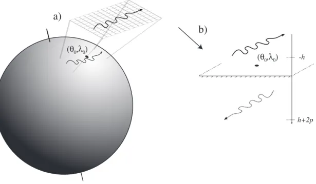
The following process was used to compute the induced electromagnetic fields at the surface of the Earth (see Fig. 2): 1.) Ionospheric currents produced by the BATS-R-US were transformed from geomagnetic coordinates to geographic co-ordinates (GEO). 2.) A point (θ0, λ0) in GEO was selected

to which fields are computed. 3.) Horizontal ionospheric currents within a radius of 1000 km about (θ0, λ0) were

de-termined for each time step. Note that as in the auroral re-gion ionospheric currents close to (θ0, λ0) typically dominate

the external ground magnetic field fluctuations at (θ0, λ0),

computationally very expensive inclusion of the entire iono-sphere is not necessary. 4.) The time series of the hori-zontal ionospheric currents within radius of 1000 km about (θ0, λ0) were transformed to Cartesian coordinates using the

20 30 40 50 60 70 80 90 100 110 120 0 20 40 60 80 Ion dens. [cm −3 ] 20 30 40 50 60 70 80 90 100 110 120 0 5 10 15 x 105 Temp. [K] 20 30 40 50 60 70 80 90 100 110 120 −800 −600 −400 V x [km/s] 20 30 40 50 60 70 80 90 100 110 120 −20 0 20 B y [nT] 20 30 40 50 60 70 80 90 100 110 120 −10 0 10 20 30 B z [nT] UT [h]

Fig. 1. The solar wind driver of the BATS-R-US run. The time is UT hours from the beginning of 24 October 2003. The vertical dashed

lines indicate the beginning of each new UT day and the solid straight line in the bottom panel indicates the zero-level.

stereographic projection and the currents were interpolated to a uniform rectangular Cartesian grid. 5.) Additional currents carrying out the current essentially from and to infinity were added to the edges of the Cartesian grid. This step is neces-sary to avoid the strong artificial field-aligned currents at the edges of the grid. The additional currents eliminate the field-aligned currents at the edges completely. 6.) The Complex Image Method (CIM) (Boteler and Pirjola, 1998; Pirjola and Viljanen, 1998) was used to compute the ground response to the ionospheric driving with given one-dimensional

(1-D) ground conductivity structure. In using CIM we assume that field-aligned currents are exactly vertical and we de-compose the ionospheric currents into U-shaped current ele-ments; field-aligned currents at the two points of the Carte-sian grid and a horizontal current filament with equal current amplitude in between these points. CIM computations are carried out in the spectral domain, transformations between the temporal and the spectral domains were carried out using Fast Fourier Transformation.

h+2p -h

a)

b)

(θ฀,λ฀)

(θ฀,λ฀)

Fig. 2. Schematic view to the key steps for computing geomagnetically induced electromagnetic fields from the ionospheric output of the

global MHD codes. (a) The time series of the horizontal ionospheric currents within a radius of 1000 km about (θ₀, λ₀) are transformed to Cartesian coordinates using the stereographic projection and the currents are interpolated to a uniform rectangular grid. (b) image of the original current system at the height h is placed to the depth h+2p. p is the complex depth determined using the 1-D conductivity structure of the Earth (Pirjola and Viljanen, 1998). The total field at (θ0, λ0) is a superimposition of the fields produced by the original current at

height h and the image current at depth h+2p.

The process used to compute the induced electromagnetic fields contains simplifications that require some discussion. First, only the local (within radius of 1000 km) ionospheric current variations are used to drive the geomagnetic induc-tion. Although this is a generally valid approach for the au-roral ionosphere which is relatively close to the surface of the Earth, the same simplification cannot be used if more distant currents, for example the ring current, are used. However, as was mentioned above, inclusion of currents from large ar-eas is computationally expensive and thus minimization of the space over which the integration is made is preferable. Also the usage of the Cartesian geometry requires spatial locality; a part of the surface of the sphere having a ra-dius of RE cannot really be described as a plane for

dis-tances greater than about 1000 km. Additionally, we need to assume that the field-aliged currents are exactly vertical (Pirjola and Viljanen, 1998). This is a generally valid as-sumption in auroral ionospheric studies (e.g., Untiedt and Baumjohann, 1993) but the same is not true for lower lati-tudes where the inclination of the currents is far from ver-tical. Finally, at present CIM is formulated to be applica-ble only to studies where the ground conductivity is 1-D, i.e. there are no horizontal conductivity gradients. Although 1-D approximation has been shown to be valid in numerous space weather-related geomagnetic induction studies (see e.g., Vil-janen et al., 2004; Pulkkinen and Engels, 2005), there are important special cases where horizontal gradients cannot be

neglected. Such cases include, for example, boundaries of continents and deep oceans where the so-called “coast effect” plays an important role in modifying the induced electromag-netic fields (e.g., Beamish et al., 2002; Olsen and Kuvshinov, 2004). Due to the relatively shallow sea-shores, the close proximity of the sea to some of the ground magnetometer stations used in this study does not severely distort the valid-ity of the 1-D approximation. Note that 1-D model can be varied as a function of (θ0, λ0), which enables approximate

treatment of lateral variations in the ground response. What follows from the considerations above is that the procedure used to compute the induced electromagnetic fields is tailored for auroral ionospheric studies; a more general approach is necessary for other types of iono-spheric/magnetospheric input. However, in the context of space weather, as the most intense induced fields and thus also the greatest technological hazards are experienced in the auroral regions, the simplified approach is justified. More-over, the 1-D approach that neglects horizontal gradients of the ground conductivity is numerically much lighter than, for example, full 3-D geomagnetic induction modeling (see e.g., Avdeev et al., 2002). This is obviously beneficial if possi-ble operational activities are kept in mind. Anyway, with the introduced modeling process the numerical bottleneck is the magnetospheric MHD, not the computations associated with the geomagnetic induction.

3 24–29 October 2003 event and the qualitative valida-tion of the model performance

The geomagnetically active period of 24–29 October 2003 was a prelude for the extremely intense Halloween storms of 29–31 October 2003 (for a GIC view to the storm, see Pulkki-nen et al., 2005). However, despite the storm strength of the period of our interest was significantly smaller than that of the Halloween storms, there was notable auroral ionospheric activity throughout 24–29 October 2003 as will be seen be-low. It follows, that the period is of interest also from the space weather viewpoint. In addition, it is quite clear that ex-treme storms require exex-treme model performance and thus it is worthwhile to start the modeling and the subsequent anal-ysis with more moderate challenges.

The solar wind driver of the MHD code is shown in Fig. 1. It is seen that especially in terms of the Bz component of

the interplanetary magnetic field (IMF), the driving was only moderate. However, there were several negative “sweeps” of Bz each causing enhanced ionospheric activity. This is

true especially at the end of the event where the increasing solar wind speed and highly fluctuating but on average neg-ative Bz, the beginning of the Halloween storm sequence,

causes already quite notable ionospheric activity. It should be noted that L1 solar wind plasma observations, especially proton density recordings contain significant inaccuracies for the Halloween storm event (Skoug et al., 2004; Dmitriev et al., 2005). These problems, however, affect our analysis only at the very end of the period (starting from about 11:00 UT in Fig. 1) where the solar velocity and density are uncertain. The points (θ0, λ0) on the ground at which we compute the

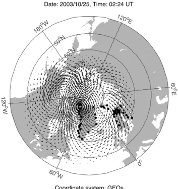
modeled fields are shown in Fig. 3. These are the locations from which we obtained measured ground magnetic field data to be used in analyzing the model performance. Figure 3 also shows a snapshot of the ionospheric output of the BATS-R-US. From this one of the shortcomings of the model run becomes apparent: the inner magnetospheric boundary of 3 REmapped to the ionosphere along the magnetic field lines

does not extend very low in magnetic latitude. This should be considered as a relatively serious setback as during the most intense storms the auroral oval and corresponding iono-spheric fluctuations causing large GIC expand to latitudes well below the lower boundary mapped from 3 RE (for an

extreme case, see Tsurutani et al., 2003). Although, for com-putational reasons, it may not be feasible to push the inner boundary of the MHD much below 3 RE, this is the first

ob-vious issue that needs to be addressed to enhance the usabil-ity of the global magnetospheric MHD for storm-time GIC modeling. This matter will be investigated in detail in the forthcoming studies that will include inner magnetospheric physics modules to the modeling chain.

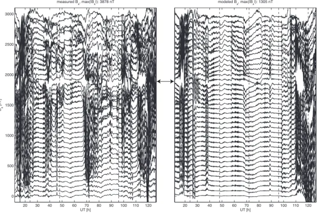
In Fig. 4 we present the x-component (geographic north) of the measured and the modeled magnetic field fluctuations at the stations shown in Fig. 3. Note that the modeled fields are not only due to the external sources but via the process

1₂ 0_o W 60o W 0 o 6₀ o E 120o E 180 oW 50 oN 60 oN 70 o_N 80 o_N Date: 2003/10/25, Time: 02:24 UT

Coordinate system: GEOs

Fig. 3. Snapshot of the horizontal ionospheric currents given by

the BATS-R-US. Dots indicate the locations to which the ground fields are computed and from which the measured ground magnetic field data was obtained. The date and the time of the snapshot is indicated in the title of the figure.

described in the previous section, also the internal contribu-tions are included now. As a first-order approximation, the same conductivity model of central Finland (e.g., Viljanen et al., 1999) was used for all stations; other conductivity models can be added later.

The complex multiscale nature of auroral geomagnetic fluctuations is clearly seen in Fig. 4: wide variety of tem-poral and spatial scales are present in both the measured and the modeled data. The multiscale nature of the fluctu-ations makes a good visual presentation of the raw time se-ries difficult as smaller scale features tend to smear the larger scale behavior. Thus, to better show the behavior at larger scales, we carried out moving average filtering (with moving 120 min windows) of the data in Fig. 4. The filtered data is shown in Fig. 5.

The first general observation from Figs. 4 and 5 is that although at the end of the event the model chain fails to re-produce the extreme amplitudes of the measured magnetic field fluctuations (maximum of 3673 nT), possibly associated with a substorm-type activity, the modeled field amplitudes seem to match to some extent with the measured field am-plitudes. However, it is easily seen that the measured mag-netic field appears to be more disturbed than the modeled field. Exceptions to this are the fluctuations at the beginning and at the end of the event where also the model produces very disturbed fields. By comparing the modeled magnetic

20 30 40 50 60 70 80 90 100 110 120 0 500 1000 1500 2000 2500 3000 UT [h] Bx [n T] modeled Bx, max(|Bx|): 1305 nT 20 30 40 50 60 70 80 90 100 110 120 0 500 1000 1500 2000 2500 3000 UT [h] Bx [n T] measured Bx, max(|Bx|): 3878 nT

Fig. 4. The x-component (geographic north) of the measured (left panel) and the modeled (right panel) magnetic field fluctuations at stations

shown in Fig. 3. Arrow in between the panels shows the separation between stations west of the Greenwich meridian (up from the arrow) and east of the Greenwich meridian (down from the arrow). Both sets are arranged from the geographically southernmost (bottom) to the northernmost (top) station. The time is UT hours from the beginning of 24 October 2003. The vertical dashed lines indicate the beginning of each new UT day.

fluctuations to the solar wind driver in Fig. 1, it is seen that the source for these, possibly global magnetospheric fluctua-tions is the highly turbulent IMF.

Another possible problem with the MHD-based modeling is underlined by the activity observed around hour 70 after 24 October, 00:00 UT seen in Figs. 4 and 5, which is to a large extent absent in the modeled time series. It should be noted that as at least part of the observed activity around hour 70 may be associated with substorm-type physical processes, which may be partially non-MHD, this particular activity may be out of the scope of global MHD modeling (more discussion about this below). Anyhow, despite the obvious differences, we conclude that the overall visual spatiotempo-ral morphology of the measured and the modeled magnetic field fluctuations seems to be quite similar.

We then move to take a look at the geomagnetically in-duced electric fields and currents. First, we model the “mea-sured” electric field with the plane wave method (Cagniard, 1953) by using the measured ground magnetic field fluctua-tions and the ground conductivity model of central Finland. In the absence of steep lateral ground conductivity gradi-ents, the electric field modeled this way corresponds rela-tively closely to the actual meso-scale (∼100 km) field (see

e.g., Viljanen et al., 2004). In fact, the modeled electric field is often more representative of the meso-scale fields for GIC-related applications than the real measured electric field. The reason for this is that the electric field measurements using electrode distances of the order of hundreds of meters is of-ten significantly distorted by the local inhomogeneities of the ground conductivity. Such distortions tend to smear the electric field of our interest and thus generally such measure-ments are of no use in GIC studies.

Once we have obtained both the modeled and the “mea-sured” electric fields at the stations shown in Fig. 3, we insert them into the equation

GIC = aEx+bEy (1)

where Exand Eyare the horizontal components of the

elec-tric field and a and b are constant coefficients. Equation (1) is used to model GIC fluctuations in technological systems when the local electric field is known. The coefficients a and b depend on the electrical, geometrical and topological properties of the system of interest and they can be deduced empirically and/or theoretically (Lehtinen and Pirjola, 1985; Pulkkinen et al., 2001a, 2006b). We will use coefficients

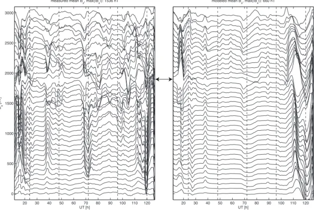
20 30 40 50 60 70 80 90 100 110 120 0 500 1000 1500 2000 2500 3000 UT [h] Bx [n T]

modeled mean B_x, max(|B_x|): 660 nT

20 30 40 50 60 70 80 90 100 110 120 0 500 1000 1500 2000 2500 3000 UT [h] Bx [n T]

measured mean B_x, max(|B_x|): 1536 nT

Fig. 5. Average magnetic field fluctuations for data shown in Fig. 4. The averaging was carried out in moving windows having length of

120 min.

for the M¨ants¨al¨a section of the Finnish natural gas pipeline (Pulkkinen et al., 2001b). By using the same ground conduc-tivity model and the same coefficients a and b, we essentially assume that the ground and the network conditions are identi-cal for all stations which is, of course, a crude approximation. However, as our primary interest at this point is in testing the capability of the MHD to produce realistic ionospheric cur-rent fluctuations driving the geomagnetic induction process, the approach can be considered acceptable.

At this point we re-emphasize that due to the 4-min tem-poral resolution of the MHD data, all data presented here are averaged to the 4-min resolution. As was shown by Pulkki-nen et al. (2006b), temporal averaging of the magnetic field data beyond of about 1-min resolution may reduce the capa-bility of the data to produce the highest GIC peaks; our rough estimation is that averaging to the 4-min resolution may re-duce the peak values of the computed auroral GIC to about 50 per cent of their 10-s values. Thus, in the future mod-eling efforts one should prefer the usage of higher temporal resolution MHD data.

In Fig. 6 we show the “measured’ and the modeled GIC at all stations. It is again seen that the multiscale nature of the fluctuations makes good visual presentation of the raw data difficult. As the noise-like character of GIC makes compu-tation of the 120 min averages quite meaningless, we char-acterize the fluctuations by computing moving standard

de-viation (with moving 120 min windows) of the data instead. The results of these computations are shown in Fig. 7.

The basic observations from Figs. 6 and 7 are similar to those from Figs. 4 and 5: although the peak values are smaller, the modeled GIC can obtain amplitudes comparable to those of the “measured” GIC and the basic spatiotemporal morphology of GIC is quite similar. Taking into account the more disturbed measured field in Fig. 4 and the fact that the time derivative of the magnetic field is a quite good proxy for the GIC activity (Viljanen et al., 2001), the morpholog-ical correspondence between the GIC can be considered, in the context of complex auroral ionospheric phenomena, quite good. From the qualitative viewpoint, we may conclude that for this particular event and with this particular model setup, the global magnetospheric MHD seems to be able to repro-duce some of the basic features of GIC.

4 Utility metrics-based quantitative validation of the

model performance

Next we want to transfer the qualitative view of Figs. 4–7 into a quantitative one. Here we need to put some special consideration for appropriate metrics. We note that this part of the study builds on the work by Weigel et al. (2006) (and

20 30 40 50 60 70 80 90 100 110 120 0 20 40 60 80 100 UT [h] G IC [A]

modeled GIC, max(|GIC|): 41 A

20 30 40 50 60 70 80 90 100 110 120 0 20 40 60 80 100 UT [h] G IC [A]

"measured" GIC, max(|GIC|): 129 A

Fig. 6. “Measured” (see the text for explanation) and the modeled GIC at stations shown in Fig. 3. Arrow in between the panels shows the

separation between stations west of the Greenwich meridian (up from the arrow) and east of the Greenwich meridian (down from the arrow). Both sets are arranged from the geographically southernmost (bottom) to the northernmost (top) station. The time is UT hours from the beginning of 24 October 2003. The vertical dashed lines indicate the beginning of each new UT day.

references therein) and the reader is referred there for more details on the discussed metrics.

In physics, by far the most popular metrics are correlation-based, like that of the mean squared difference. Such metrics are particularly suitable for, for example, model optimization due to their convenient mathematical properties. However, in our case these basic metrics are not ideal for two differ-ent reasons: 1.) due to the complexity of the GIC signal and 2.) due to the lack of user-relevance. As can be qualitatively seen from Fig. 6 and as has been quantitatively verified for the time derivative of the ground magnetic field fluctuations by Pulkkinen et al. (2006a), the GIC signal is very complex. In fact, some of the statistical properties of the signal resem-ble that of the white noise. It follows, that for such highly fluctuating signal, for example, linear correlation may not be a “fair” metric for evaluating the model performance. Thus, a metric focusing on some more overall aspect of the signal, like mere amplitude, should be preferred. On the other hand, from the viewpoint of the user, one should prefer metrics that has something to do with the actual decision process involv-ing the forecast → mitigation action.

Quite conveniently, both of the aforementioned issues are addressed by the so-called utility metrics. The utility of the

forecast is defined as

Uf =BNH−CNH (2)

where NHis the number of correct forecasts, NHis the

num-ber of false alarms, C is the cost of taking mitigating ac-tion and B is the benefit from having taken mitigating acac-tion when an event occurred. In using this particular metric we assume that 1.) the user takes the same mitigating action fol-lowing each forecast of an event, 2.) an “always mitigate” strategy yields a net monetary loss for the user and 3.) the user seeks to maximize the monetary gain Uf. Note that

sometimes it may be preferable for the user to change the system in a way that removes the threat altogether thus vi-olating the assumption no. 2. Although such actions can be carried out to mitigate GIC (Molinski, 2002), often the costs of changing the system cannot be justified by the size of the threat posed by GIC. Then the assumption no. 2 holds and it may be beneficial for the user to seek for monetary gain

Uf in terms of GIC forecasts. Also note that we are

consid-ering utility with respect to a system that is never mitigated, which is the case for most of the systems experiencing GIC. In another words, we are considering the difference between losses/gains experienced by the two systems. It follows that we do not need to consider missed events; a missed event will

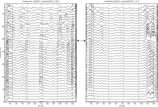
20 30 40 50 60 70 80 90 100 110 120 0 10 20 30 40 50 60 70 UT [h] st d(G IC ) [ A]

modeled std(GIC), max(std(GIC)): 12 A

20 30 40 50 60 70 80 90 100 110 120 0 10 20 30 40 50 60 70 UT [h] st d(G IC ) [ A]

"measured" std(GIC), max(std(GIC)): 38 A

Fig. 7. Standard deviation of GIC data in Fig. 6. The standard deviation was computed for moving windows having length of 120 min.

cause the same monetary loss for both the reference system and the system using mitigation actions.

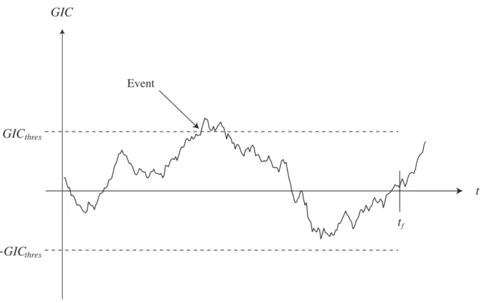
In using the utility, we evaluate the model performance in terms of its capability to predict “events”. Here we define an event as follows: within a forecast window 0≤t ≤tf, the

absolute value of GIC exceeds event threshold |GICthres|(see

Fig. 8). The windows are moved over the time series in non-overlapping parts and events for given tf and |GICthres|are

recorded for both the measured and the modeled GIC. As values for B and C in Eq. (2) are system dependent and are estimated by the user, rather than computing Uf, we

com-pute the forecast ratio Rf=NH/NH. It is easily seen that the

utility Uf is positive if Rf>C/B and thus by reporting Rf

of the forecast the user can quantify the utility of the forecast once the values B and C and are known. In model compar-isons, a model with a larger Rf will have a greater utility

Uf.

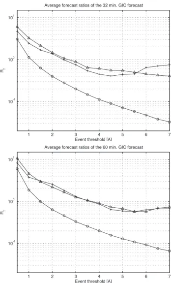
In Fig. 9 we show Rf for the modeled GIC and for two

different persistence models/rules as a function of |GICthres|

for tf=32 min and tf=60 min. The persistence models are:

1.) “always an event forecast”, i.e. during disturbed periods the alarm is always on. Note that this is not necessarily the same as taking mitigation action always; during quiet condi-tions the system may not be at the state of GIC mitigation. The alarm is switched on, for example, only when an ap-proaching interplanetary coronal mass ejection is observed.

2.) “nearest neighbor forecast”, i.e. the forecast for the next forecast window will be the same as the observation for the previous one. Rf were computed separately for each station,

we show here only the average taken over all of the stations. It is noted that there are differences in Rf between different

stations especially as a function of the latitude. However, the basic trend is the same for all stations and thus the average

Rf gives a quite good idea about the overall model

perfor-mance.

As seen from Fig. 9, the forecast ratios behave sim-ilarly for both 32- and 60-min forecast windows. The only clear difference is that the utility tends to be slightly higher for the 60-min forecasts with smaller event thresh-old (|GICthres|<5 A). Interestingly, for event thresholds

|GICthres|>5.5 A, the MHD-based forecasts have the greatest

utility for 32-min forecasts. In general, it is seen that the first-principles modeling process is capable of producing equal, and in some cases even superior economic benefit to that of the used persistence models. Considering the potential for improving the modeling accuracy by adding new model com-ponents and by using higher spatial resolution in the global magnetospheric MHD, this result is promising. Whether or not the potential can be realized, will be investigated in the continuation of this work.

t

GIC

-

GIC

GIC

t

Event

Fig. 8. The determination of an “event” from the GIC time series. The event is defined as a crossing of the event threshold |GICthres|within

a forecast window 0≤t ≤tf.

5 Summary and discussion

Empirical modeling of the ground magnetic field fluctua-tions, which via Faraday’s law of induction are closely re-lated to the geomagnetically induced electromagnetic fields and currents, has long traditions in the modern space physics (e.g., Bargatze et al., 1985; Vassiliadis et al., 1995; Valdivia et al., 1999; Weimer, 2005). These efforts have not been in vain; there has been great success in predicting some over-all aspects of geomagnetic field fluctuations, like those of the global geomagnetic indices, and the models have been able to give crucial insights into the physical characteristics of the solar wind-magnetosphere-ionosphere system. However, ac-curate prediction of the geomagnetic induction-related field fluctuations requires going beyond the overall aspects. More specifically, one needs to know the rate of the change of the ground magnetic field at the temporal scales of the order of minutes; as the variations around the mean are usually more complex than the mean behavior itself, it is thus quite clear that extracting such information poses a new challenge for the geomagnetic field modeling. Importantly, some recent empirical modeling efforts have had some success in pre-dicting the rapidly fluctuating part of the geomagnetic field (Weigel et al., 2003; Wintoft, 2005). These models naturally have potential for usage in space weather forecasting appli-cations.

As the empirical models have been “taught” to reproduce the measurements, it is clear that in some situations the em-pirical models outperform the first-principles models. How-ever, in situations that the empirical models have not “seen”, they may extrapolate very poorly whereas first-principles models always, in principle, produce physically reasonable results provided that the basic physics of the system remain unchanged. This is especially important in rare and extreme situations that naturally in the context of space weather are of the utmost importance (see also, Lopez et al., 2007). From the physics viewpoint, the performance of our first-principles models is the ultimate test for our understanding of the solar wind-magnetosphere-ionosphere system; the system’s evolu-tion equaevolu-tions are derived using our understanding of the un-derlaying elementary physical principles rather than by the data.

The point of the above discussion is, while acknowl-edging the great significance of the empirical modeling ef-forts, to emphasize the importance of pursuing towards first-principles-based modeling of the solar wind-magnetosphere-ionosphere system. Accordingly, the goal of this work was to carry out first-principles-based modeling of near-space phe-nomena from the upstream solar wind to the surface of the Earth. More specifically, we introduced a basic modeling procedure for obtaining the geomagnetically induced elec-tromagnetic fields and currents from the output of global

magnetospheric MHD codes. We also presented metrics that take into account both the complex nature of the signal and possible forecasting applications of the modeling process. The modeling process and the metrics were introduced with the help of an actual example space weather event of 24– 29 October 2003. Observations of the ground magnetic field fluctuations were used to carry out preliminary tests of the performance of the model chain. As space weather applica-tions are the main motivation of the study, the performance tests were focused on GIC.

It was seen that for the studied event, some central features of the overall ionospheric current fluctuations associated with GIC were captured by the modeling process. More specif-ically, the basic spatiotemporal morphology of the modeled and “measured” GIC was quite similar. Furthermore, the pre-sented user-relevant utility metrics demonstrated that global MHD-based modeling can outperform simple GIC persis-tence models. We may thus conclude that considering the relatively modest model setup, the first results are encourag-ing.

It should be noted, however, that despite the success in re-producing some of the observed features of the GIC-related ionospheric current fluctuations, there were also important shortcomings. First, the 3 RE inner magnetospheric

bound-ary of the global MHD run does not extend very low in mag-netic latitude in the ionosphere. This is a setback as dur-ing strong storms, in addition to generally very disturbed polar regions, the auroral oval with highly fluctuating iono-spheric currents generating large GIC may expand below the ionospheric MHD boundary. However, this problem may be scaled back by pushing the inner boundary of the global MHD closer to the Earth and by including inner magneto-spheric model to the modeling chain. Inclusion of the in-ner magnetosphere may be important also in terms of having more realistic dynamics associated with the region 2 current system (e.g., De Zeeuw et al., 2004).

It is emphasized that realistic modeling of the ionospheric currents is perhaps the most important factor influencing the accuracy of the computed induced fields. Thus, it is ob-vious that inclusion of as many as possible central physi-cal elements contributing to the magnetosphere-ionosphere coupling is highly desirable. However, it is clear that some physics may be missing partially or altogether in the MHD-based description of the system; also this was demonstrated in the example event. For example, it is well-known that some processes in the plasma sheet are beyond the scope of MHD. Furthermore, these processes may play a crucial role, for example, in the substorm phenomenon which is known to be statistically one of the most important causes for large high-latitude GIC (e.g., Viljanen et al, 2006a). Although there is evidence that global MHD can produce substorm-like behavior of the magnetosphere (e.g., Raeder et al., 2001a; Wiltberger et al., 2005), it is all but clear if the highly com-plex nature of the ground magnetic field variations associated with substorms (for a quantification of this complexity, see

1 2 3 4 5 6 7

10-1 100 101

Event threshold [A] Rf

Average forecast ratios of the 32 min. GIC forecast

1 2 3 4 5 6 7

10-1 100 101

Event threshold [A] Rf

Average forecast ratios of the 60 min. GIC forecast

Fig. 9. Forecast ratios NH/N_H of the modeled GIC (plusses) and

persistence models 1 (circles) and 2 (triangles) as a function of the event threshold |GICthres|. Top panel: forecast window tf of 32 min

was used. Bottom panel: forecast window tf of 60 min was used.

Pulkkinen et al., 2006a) can be reproduced by basic global magnetospheric MHD models (for an alternative approach, see e.g., Klimas et al., 2004). Obviously, capturing these ex-treme variations is very important from the GIC viewpoint.

As mentioned above, the work at hand comprises Phase 1 of the project in which we test the present capabilities of first-principles modeling of space weather from the ground viewpoint. In the follow-up, we will utilize numerous setups and combinations of the models hosted by the Community Coordinated Modeling Center (CCMC) operating at NASA Goddard Space Flight Center to find the optimal way to carry out the modeling. The optimization will be carried out by ap-plying user-relevant metrics, like that of the presented utility metrics.

Acknowledgements. A. Viljanen and J. Waterman of Finnish Me-teorological Institute and Danish MeMe-teorological Institute, respec-tively, are acknowledged for providing the IMAGE and Greenland magnetometer array data utilized in this study. Comments on the manuscript by A. Viljanen and R. Pirjola are greatly acknowledged. CIM software by A. Viljanen was used in this work.

Topical Editor M. Pinnock thanks J. Watermann and S. G. Shep-herd for their help in evaluating this paper.

References

Avdeev, D. B., Kuvshinov, A. V., Pankratov, O. V., and Newman, O. G.: Three-dimensional induction logging problems, Part I: An integral equation solution and model comparisons, Geophysics, 67, 2, 413–426, 2002.

Bargatze, L. F., Baker, D. N., McPherron, R. L., and Hones, E. W.: Magnetospheric impulse response for many levels of geomag-netic activity, J. Geophys. Res., 90(A7), 6387–6394, 1985. Bargatze, L. F., McPherron, R. L., Minamora, J., and Weimer,

D.: A new interpretation of Weimer et al.’s solar wind prop-agation delay technique, J. Geophys. Res., 110, A07105, doi:10.1029/2004JA010902, 2005.

Beamish, D., Clark, T. D. G., Clarke, E., and Thomson, A. W. P.: Geomagnetically induced currents in the UK: geomagnetic vari-ations and surface electric fields, J. Atmos. Sol. Terr. Phys., 64, 1779–1792, 2002.

Bolduc, L.: GIC observations and studies in the Hydro-Qubec power system, J. Atmos. Solar-Terr. Phys., 64, 16, 1793–1802, 2002.

Boteler, D. H. and Pirjola, R. J.: The complex-image method for calculating the magnetic and electric fields produced at the sur-face of the Earth by the auroral electrojet, Geophys. J. Int., 132, 1, 31–40, 1998.

Boteler, D. H., Pirjola, R. J., and Nevanlinna, H.: The Effects of Geomagnetic Disturbances on Electrical Systems at the Earth’s Surface, Adv. Space Res., 22, 17–27, 1998.

Boteler, D. H., Trichtchenko, L., Pirjola, R., Parmelee, J., Souksaly, S., Foss, A., and Marti, L.: Real-time simulation of geomagneti-cally induced currents, Proceedings of the Canadian Conference on Electrical and Computer Engineering, IEEE Canada, Ottawa, Ontario, Canada, 7–10 May 2006, 4 pp, 2006.

Cagniard, L.: Basic theory of the magneto-telluric method of geo-physical prospecting, Geophysics, 18(3), 605–635, 1953. Czech, P., Chano, S., Huynh, H., and Dutil, A.: The Hydro-Qu´ebec

System Blackout of 13 March 1989: System Response to Geo-magnetic Disturbance, EPRI Report, TR-100450, Proceedings of Geomagnetically Induced Currents Conference, Millbrae, Cali-fornia, USA, 8–10 November 1989, 1992.

De Zeeuw, D. L., Sazykin, S., Wolf, R. A., Gombosi, T. I., Ridley, A. J., and T´oth, G.: Coupling of a global MHD code and an inner magnetospheric model: Initial results, J. Geophys. Res., 109, A12219, doi:10.1029/2003JA010366, 2004.

Dmitriev, A. V., Chao, J.-K., Suvarova, A. V., Ackerson, K., Ishisaka, K., Kasaba, Y., Kojima, H., and Matsumoto, H.: Indirect estimation of the solar wind conditions in 29–31 October 2003, J. Geophys. Res., 110, A09S02, doi:10.1029/2004JA010806, 2005.

Klimas, A. J., Uritsky, V. M., Vassiliadis, D., and Baker, D. N.: Reconnection and scale-free avalanching in a

driven current-sheet model, J. Geophys. Res., 109, A02218, doi:10.1029/2003JA010036, 2004.

Lehtinen, M. and Pirjola, R.: Currents produced in earthed conduc-tor networks by geomagnetically-induced electric fields, Ann. Geophys., 3(4), 479–484, 1985.

Lopez R. E., Hernandez, S., Wiltberger, M., Huang, C.-L., Kepko, E. L., Spence, H., Goodrich, C. C., and Lyon, J. G.: Predicting magnetopause crossings at geosynchronous or-bit during the Halloween storms, Space Weather, 5, S01005, doi:10.1029/2006SW000222, 2007.

Molinski, T.: Why utilities respect geomagnetically induced cur-rents, J. Atmos. Sol-Terr. Phys., 64, 1765–1778, 2002.

Olsen, N. and Kuvshinov, A.: Modeling the ocean effect of geo-magnetic storms, Earth Planets Space, 56, 525–530, 2004. Pirjola, R. and Viljanen, A.: Complex image method for calculating

electric and magnetic fields produced by and auroral electrojet if finite length, Ann. Geophys., 16, 1434–1444, 1998,

http://www.ann-geophys.net/16/1434/1998/.

Pirjola, R., Viljanen, A., Pulkkinen, A., Kilpua, S., and Amm, O.: Space weather effects on electric power transmission grids and pipelines, NATO Science Series, Volume “Effects of Space Weather on Technology Infrastructure”, Kluwer Academic Pub-lishers B.V., edited by: Daglis, I., Chapter 13, 235–256, 2004. Powell, K. G., Roe, P. L., Linde, T. J., Gombosi, T. I., and

De Zeeuw, D. L.: A solution-adaptive upwind scheme for ideal magnetohydrodynamics, J. Comput. Phys., 154(2), 284, doi:10.1006/jcph.1999.6299, 1999.

Pulkkinen, A., Pirjola, R., Boteler, D., Viljanen, A., and Yegorov, I.: Modelling of space weather effects on pipelines, J. Appl. Geo-phys., 48, 233–256, 2001a.

Pulkkinen, A., Viljanen, A., Pajunp¨a¨a, K., and Pirjola, R.: Record-ings and occurrence of geomagnetically induced currents in the Finnish natural gas pipeline network, J. Appl. Geophys., 48, 219–231, 2001b.

Pulkkinen, A. and Engels, M.: The role of 3D geomagnetic induc-tion in the determinainduc-tion of the ionospheric currents from the ground geomagnetic data, Ann. Geophys., 23, 909–917, 2005, http://www.ann-geophys.net/23/909/2005/.

Pulkkinen, A., Lindahl, S, Viljanen, A., and Pirjola, R.: Geomag-netic storm of 2931 October 2003: GeomagGeomag-netically induced cur-rents and their relation to problems in the Swedish high-voltage power transmission system, AGU Space Weather, 3, S08C03, doi:10.1029/2004SW000123, 2005.

Pulkkinen, A., Klimas, A., Vassiliadis, D., Uritsky, V., and Tan-skanen, E.: Spatiotemporal scaling properties of the ground geomagnetic field variations, J. Geophys. Res., 111, A03305, doi:10.1029/2005JA011294, 2006a.

Pulkkinen, A., Viljanen, A., and Pirjola, R.: Estimation of geomag-netically induced current levels from different input data, Space Weather, Vol. 4, S08005, doi:10.1029/2006SW000229, 2006b. Raeder, J., McPherron, R. L., Frank, L. A., Kokubun, S, Lu, G.,

Mukai, T., Paterson, W. R., Sigwarth, J. B., Singer, H. J., and Slavin, J. A.: Global simulation of the Geospace Environment Modeling substorm challenge event, J. Geophys. Res., 106(A1), 381–396, doi:10.1029/2000JA000605, 2001a.

Raeder, J., Wang, Y., Fuller-Rowell, T., and Singer, H. J.: Global simulation of space weather effects of the Bastille Day storm, Solar Physics, 204, 325, 2001b.

control of the magnetospheric configuration: Conductance, Ann. Geophys., 22, 567–584, 2004,

http://www.ann-geophys.net/22/567/2004/.

Skoug R. M., Gosling, J. T., Steinberg, J. T., McComas, D. J., Smith, C. W., Ness, N. F., Hu, Q., and Burlaga, L. F.: Extremely high speed solar wind: 29–30 October 2003, J. Geophys. Res., 109, A09102, doi:10.1029/2004JA010494, 2004.

T´oth, G., Sokolov, I., Gombosi, T., Chesney, D., Clauer, C.R., De Zeeuw, D., Hansen, K., Kane, K., Manchester, W., Oehmke, R., Powell, K., Ridley, A., Roussev, I., Stout, Q., Volberg, O., Wolf, R., Sazykin, S., Chan, A., Yu, B., and K´ota, J.: Space Weather Modeling Framework: A new tool for the space science community, J. Geophys. Res., 110, A12226, doi:10.1029/2005JA011126, 2005,

Tsurutani B. T., Gonzalez, W. D., Lakhina, G. S., and Alex, S.: The extreme magnetic storm of 12 September 1859, J. Geophys. Res., 108(A7), 1268, doi:10.1029/2002JA009504, 2003.

Untiedt, J. and Baumjohann, W.: Studies of polar current systems using the IMS Scandinavian magnetometer array, Space Sci. Rev., 63, 245–390, 1993.

Valdivia, J. A., Vassiliadis, D., Klimas, A., Sharma, A. S., and Papadopoulos, K.: Spatiotemporal activity of mag-netic storms, J. Geophys. Res., 104(A6), 12 239–12 250, 10.1029/1999JA900152, 1999.

Vassiliadis, D., Klimas, A. J., Baker, D. N., and Roberts, D. A.: A description of the solar wind-magnetosphere coupling based on nonlinear filters, J. Geophys. Res., 100(A3), 3495–3512, doi:10.1029/94JA02725, 1995.

Weigel, R. S., Klimas, A. J., and Vassiliadis, D.: Solar wind coupling to and predictability of ground magnetic fields and their time derivatives, J. Geophys. Res., 108(A7), 1298, doi:10.1029/2002JA009627, 2003.

Weigel, R. S., Detman, T., Rigler, E. J., and Baker, D. N.: Deci-sion theory and the analysis of rare event space weather forecasts, Space Weather, 4, S05002, doi:10.1029/2005SW000157, 2006. Weimer, D. R.: Predicting surface geomagnetic variations

us-ing ionospheric electrodynamic models, J. Geophys. Res., 110, A12307, doi:10.1029/2005JA011270, 2005.

Wiltberger, M., Elkington S. R., Guild, T., Baker, D. N., and Lyon, J. G.: Comparison of MHD simulations of isolated and storm time substorms, AGU Geophysical Monograph Series, In-ner Magnetosphere: Physics and Modeling, 155, 271–281, 2005. Wintoft, P.: Study of solar wind coupling to the time difference hor-izontal geomagnetic field, Ann. Geophys., 23, 1949–1957, 2005, http://www.ann-geophys.net/23/1949/2005/.

Viljanen, A., Pirjola, R., and Amm, O.: Magnetotelluric source ef-fect due to 3D ionospheric current systems using the complex image method for 1D conductivity structures, Earth, Planets and Space, 51, 933–945, 1999.

Viljanen, A., Nevanlinna, H., Pajunp¨a¨a, K., and Pulkkinen, A.: Time derivative of the horizontal geomagnetic field as an activity indicator, Ann. Geophys., 19, 1107–1118, 2001,

http://www.ann-geophys.net/19/1107/2001/.

Viljanen, A., Pulkkinen, A., Amm, O., Pirjola, R., Korja, T., and BEAR Working Group: Fast computation of the geoelectric field using the method of elementary current systems, Ann. Geophys., 22, 101–113, 2004,

http://www.ann-geophys.net/22/101/2004/.

Viljanen, A., Tanskanen, E., and Pulkkinen, A.: Relation between substorm characteristics and rapid temporal variations of the ground magnetic field, Ann. Geophys., 24, 725–733, 2006a. Viljanen, A., Pulkkinen, A., Pirjola, R., Pajunp¨a¨a, K., Posio, P., and

Koistinen, A.: Recordings of geomagnetically induced currents and a nowcasting service of the Finnish natural gas pipeline sys-tem, Space Weather, 4, S10004, doi:10.1029/2006SW000234, 2006b.