HAL Id: hal-02152837
https://hal.archives-ouvertes.fr/hal-02152837
Submitted on 14 Nov 2019
HAL is a multi-disciplinary open access
archive for the deposit and dissemination of sci-entific research documents, whether they are pub-lished or not. The documents may come from teaching and research institutions in France or abroad, or from public or private research centers.
L’archive ouverte pluridisciplinaire HAL, est destinée au dépôt et à la diffusion de documents scientifiques de niveau recherche, publiés ou non, émanant des établissements d’enseignement et de recherche français ou étrangers, des laboratoires publics ou privés.
Annual Sediment Transport Dynamics in the Narayani
Basin, Central Nepal: Assessing the Impacts of Erosion
Processes in the Annual Sediment Budget
Guillaume Morin, Jérôme Lavé, Christian France-Lanord, Thomas Rigaudier,
Ananta Prasad Gajurel, Rajiv Sinha
To cite this version:
Guillaume Morin, Jérôme Lavé, Christian France-Lanord, Thomas Rigaudier, Ananta Prasad Gajurel, et al.. Annual Sediment Transport Dynamics in the Narayani Basin, Central Nepal: Assessing the Impacts of Erosion Processes in the Annual Sediment Budget. Journal of Geophysical Research: Earth Surface, American Geophysical Union/Wiley, 2018, 123 (10), pp.2341-2376. �10.1029/2017JF004460�. �hal-02152837�
This article has been accepted for publication and undergone full peer review but has not been through the copyediting, typesetting, pagination and proofreading process which may lead to differences between this version and the Version of Record. Please cite this article as
Annual sediment transport dynamics in the Narayani
basin, Central Nepal: assessing the impacts of erosion
processes in the annual sediment budget
Guillaume Morin1*, Jérôme Lavé1, Christian France-Lanord1, Thomas Rigaudier1,
Ananta Prassad Gajurel2, Rajiv Sinha3
1 Centre de Recherches Pétrographiques et Géochimiques (CRPG), UMR 7358
CNRS-Université de Lorraine, 15 rue Notre Dame des Pauvres, F-54500 Vandœuvre-lès-Nancy, France
2 Department of Geology, Tribhuvan University, Ghantaghar, Kathmandu, Nepal 4 Department of Earth Sciences, Indian Institute of Technology, Kanpur 208 016, India * Corresponding author: G. P. Morin: [email protected], now at Laboratoire
d’Océanographie de Villefranche sur Mer (LOV), UMR 7093, CNRS/UPMC, F-06230 Villefranche-sur-Mer Cedex, France.
Corresponding author: G. P. Morin: [email protected],
*now at Laboratoire d’Océanographie de Villefranche sur Mer (LOV), UMR 7093, CNRS/UPMC, F-06230 Villefranche-sur-Mer Cedex, France.
Key Points:
Erosion in Central Nepal is supply-limited and driven by monsoonal precipitation, which controls triggering of landslides.
Glacial and soil erosion are minor in the annual sediment budget compared to landslides.
Current erosion rates agree with long-term erosion rates, suggesting efficient buffering of these drainage systems.
Abstract
Identifying the roles of erosional processes in the denudation of mountain ranges requires a better understanding of erosional sensitivity to climatic, topographic, or lithologic controls. We analyzed erosion in the Narayani River basin (draining central Nepal, and presenting contrasted lithologic and geochemical signatures in its outcropping rocks, and a wide variety of erosional processes and climatic conditions) to assess the relative contributions of erosion processes to the annual sediment export. By combining ADCP measurements with depth profiles and daily surface samplings of the suspended load, we propose a simplified model to precisely calculate sediment fluxes at the basin outlet. We estimate an equivalent erosion rate of 1.8-0.2+0.35mm/yr for the year 2010, similar to the average
value of 1.6-0.2+0.35 mm/yr estimated from 15 years of records and long-term (~ky) denudation rates of 1.7 mm/yr derived from cosmogenic nuclides. The stability of erosion is attributed to efficient buffering behavior and spatial integration in the drainage system. Strong relations between rainfall events and the sediment export suggest that the system is mainly supply-limited. Combining physical calculation of sediment fluxes with grain size analyses and geochemical tracers (hydroxyl isotopic compositions, carbonate contents, and total organic carbon content), we estimate that glacial and soil erosion do not contribute more than 10% and a few %, respectively to the total budget, and are only detectable during premonsoon and early monsoon periods. During the monsoon, erosion by landslides and mass-wasting events overwhelms the sediment budget, confirming the dominant role of these erosional processes in active mountain chains.
1. Introduction
Mountain range landscapes and topography result from tectonic deformation and mass removal by erosion. The effects of tectonics and climate in shaping topography depend largely on the erosive processes acting at the Earth’s surface and their sensitivity to these forcings. Such erosive controls have implications at all time scales and are particularly relevant to the long-standing debate on the interactions between tectonics, climate, and erosion during orogenic construction. Comprehension and quantification of such interactions is challenging, in part due to the diversity of erosive processes (hillslope, fluvial, glacial) that occur in different parts of the landscape and are variously sensitive to climatic variables (e.g., Avouac, 2003; Gabet et al., 2004b; Bookhagen et al., 2005; Champagnac et al., 2012; Fuchs et al., 2015; Deal et al., 2017).
Because of its sustained tectonic activity and diversity of climatic conditions, the Himalayan range is a remarkable region of the world for studying the interactions between active tectonics, climate, and topography (e.g., Lavé & Avouac, 2001; Burbank et al., 2003; Clift et al., 2008; Gabet et al., 2008; Godard et al., 2014; Deal et al., 2017). The topographic step between the low Ganga plain and the highest Himalayan summits or the Tibetan Plateau acts as a barrier to atmospheric circulation and drives heavy precipitation during the Indian monsoon (Boos & Kuang, 2010; Molnar et al., 2010). Monsoonal precipitation combined with the steep Himalayan relief produces denudation rates among the highest on Earth. The system generates one of the most important sediment fluxes on the planet, feeding the Ganga plain and the Bengal fan.
Understanding how Himalayan topography and tectonics respond to climatic and erosive forcings requires a comprehensive view of active erosion in the Himalaya. This includes studying present erosional fluxes, documenting the dominant erosional processes occurring in different physiographic units of the range, and defining the response of these erosional processes to climatic forcing.
Among erosional processes, landslides have been shown to be the major erosive agent in active mountain ranges (Hovius et al., 1997; Dadson et al., 2004; Parker et al., 2015) and particularly in Himalaya, where their occurrence displays high spatial and temporal variability (Shroder, 1998). The factors that control their distribution, evolution, and behavior may be as diverse as earthquakes (Dadson et al., 2004; Meunier et al., 2008), rainstorms (Iverson, 2000; Gabet et al., 2004a), or accumulated seasonal rainfall through groundwater
saturation (Gabet et al., 2004b; Dahal & Hasegawa, 2008) which affects bedrock strength and hillslope angle of repose (Gabet et al., 2004a) as suggested by the coincident scaling of topography and precipitation observed in the steep relief of the Greater Himalaya.
Soil erosion may also play a significant role as suggested by Heimsath et al., (2012) and Larsen et al., (2014) who reported that soil production rates can be very high (up to 2.5 mm/yr) and increase to above theoretical limits with physical erosion in rapidly eroding watersheds (e.g., Gabet & Mudd, 2009). Nonetheless, those authors also reported that soil production rates represent only a fraction of catchment-wide denudation, which is largely dominated by mass wasting and landslides at the mountain scale. While in the Middle Hills of central Nepal, south of the high range, (West et al., 2015) identified that soil erosion can dominate physical erosion at the catchment scale in the absence of active landslides, such that the dominance of landslides over soil erosion remains to be shown at the scale of the entire range.
Lastly, glacial erosion is potentially more efficient than landslide erosion driven by fluvial incision (e.g., Hallet et al., 1996), although this inference was recently questioned (Thomson et al., 2010). Yet, the High Himalayan summits are covered by numerous glaciers and large U-shaped valleys of up to 3,000 m relief that attest to past glacial erosion so that Gabet et al., (2008) proposed that glacial erosion dominates in rivers draining the northern sides of the range in central Nepal, although this contribution is dwarfed by other contributions at the scale of the range because of the limited extent of glacier cover. In contrast, (Godard et al., 2012) concluded from 10Be concentrations in river sands collected in the same area that active glacial erosion can exceed the long-term erosion rate by two or three times, which leaves an imprint in downstream river sediments.
In that respect, the aim of this study is to measure the intensity of erosion and assess the relative contributions of the different erosion processes at the scale of the Himalayan range. We followed an alternative and integrative approach by studying the sediment export of a major river during an entire monsoon cycle. We characterized the fluxes and sources of the sediment transported by a major river and their relations with rainfall and temperature chronicles in central Himalaya, a region marked by strong rainfall seasonality. We explore the relative contributions and intensities of the different erosion processes in relation to climatic variables. Rather than monitoring a large number of watersheds exposed to contrasted climates and erosional processes, our approach offers the possibility of tracking
the imprint of diverse sediment sources in the same system and their responses to the seasonality of the monsoon climate.
Sediment transport in a large river and associated sedimentary bodies might result in a dampening / delaying of the original signals associated with a change in climatic or tectonic signal (Covault et al., 2010; Armitage et al., 2011; Coulthard & Van de Wiel, 2013) due to internal dynamics (Jerolmack & Paola, 2010) or the timescale of integration (Castelltort & Van Den Driessche, 2003; Armitage et al., 2011). In order to catch the initial signal, the filter associated to the sediment transport has to be limited as much as possible, for example by monitoring the sediment at the outlet of the mountain basin and before the plains. See Romans et al., (2016) for extensive review.
Hence, our method consists of analyzing the sediment load of a large river system at its outlet from the mountain range. This method offers several advantages: 1) it spatially smooths the stochastic effects of landslide mass wasting; 2) it provides an overall view on the erosion of a whole Himalayan section, including glaciated high peaks; and 3) it yields a direct interpretative framework of the chemical composition and sedimentological characteristics of sediments transported further downstream, which could help to decipher the sedimentary records of the Indo-Gangetic foreland basin or Bengal fan.
This paper focuses specifically on estimating the current physical erosion rate and its recent evolution in the Narayani River basin, one of the major rivers draining and eroding central Himalaya, and assessing the yields of each erosional process in the sediment budget. To do so, we analyzed sediment concentration chronicles, the geochemical composition of riverbanks and suspended loads, and hydrologic and meteorological datasets along the Narayani River. We present an original dataset of daily surface suspended sediment sampling from May to October 2010, a period that encompasses premonsoon, monsoon, and postmonsoon periods and about 80% of the total annual rainfall. We assess current rates of erosion by combining this dataset with occasional sediment depth sampling and an acoustic Doppler current profiler (ADCP) current velocity survey acquired during the 2011 monsoon, which allows us to build a semi-empirical model of sediment transport that integrates sediment fluxes over the river depth. We apply our model to suspended load concentration data recorded by the Department of Hydrology and Meteorology of Nepal (DHM) to document erosion rates over the past decade, which we then compare to current erosion rates reported by (Andermann et al., 2012a) and long-term denudation rates determined by cosmogenic dating (Godard et al., 2012, 2014; Lupker et al., 2012a).
Our 2010 sediment dataset includes tracers to discriminate between sediment sources, for instance grain size and geochemical characteristics including carbonate content, the hydrogen isotopic composition of hydrated silicates, and total organic carbon content. Thus, we present a multivariate analysis of the suspended load in 2010 that reveals geochemical fluctuations in relation to sediment flux and river discharge. These temporal variations are likely related to the contributions of the different erosion processes active in the basin, i.e., mainly glaciers, soils, and landslides.
2. Geologic, climatic, and geomorphologic settings
The Narayani River drains the central Nepal Himalayan range and is the most important tributary of the Ganga in terms of discharge and sediment flux (Singh et al., 2008; Andermann et al., 2012a; Lupker et al., 2012a). It drains a 32,000 km2 mountain basin whose elevation varies from 180 to 8147 m. The drainage system comprises five major tributaries from west to east: Kali Gandaki, Seti, Marsyandi, Bhuri Gandaki, and Trisuli. The Kali and Trisuli Rivers drain a part of the Tibetan plateau that corresponds to 39 and 40% of their respective basin areas. The Narayani basin drains 5 main Himalayan geologic units from north to south: 1) the Tethyan Sedimentary Series (TSS), a low-grade Palaeozoic–Eocene sedimentary series of the passive northern Indian margin that includes a large proportion of limestone and carbonates; 2) the High Himalayan Crystalline (HHC) formations, high-grade metamorphic gneisses and migmatites; 3) the High Himalayan Leucogranite (HHL), intrusive into the HHC and TSS; 4) the Lesser Himalaya (LH) formations, variably metamorphosed Indian crust material of Precambrian to Palaeozoic age; and 5) the Mio-Pliocene Siwaliks, sediments of the foreland basin exhumed by the most recent frontal thrusts (Colchen et al. 1986). According to the geologic map (Department of Mines and Geology of Nepal), the respective surface proportions of outcropping lithologies drained by the Narayani basin are ~30% TSS, ~24% High Himalayan gneisses and leucogranites (HHC+HHL), and ~46% LH units. Finally, the surface area of the Siwaliks units drained by the Narayani basin upstream of Narayanghat is negligible.
The Narayani basin is highly exposed to the monsoon, which generates a flooding season between mid-June and mid-to-late September that represents around 80% of the 1,400 1,900 mm/yr mean annual rainfall (Shrestha, et al., 2000; Bookhagen and Burbank, 2010; Andermann et al., 2011, 2012b). During the monsoon, northwestward winds bring moisture generated at the surface of the Bay of Bengal to the mountain range, generating intense
orographic precipitations. Rainfall in the Narayani basin varies greatly, with annual rainfall ranging from <50 mm in the Mustang area (the most NW part of the watershed) to ~5,000 mm south of the Annapurna Massif (Putkonen, 2004). In central Nepal, the morphologic transition from the Lesser Himalaya lowlands and Middle Hills to the High Himalaya is characterized by a sharp break in slope that forms the principal orographic barrier and stops monsoon clouds at a ~4,000 m elevation.
Consequently, the High Himalayan foothills region receives the most precipitation in Nepal (Anders et al., 2006; Bookhagen & Burbank, 2006, 2010; Andermann et al., 2011). In the Narayani basin this effect is enhanced by the relatively low elevation of the frontal Mahabharata Range, which favors cloud penetration into the interior of the range and probably explains the precipitation in front of the Annapurna Massif that is more intense than anywhere else in central Nepal. Because of the orographic barrier, the northern part of the watershed is very arid.
The High Himalayan range includes several of the highest summits in Nepal and is exposed to snowfall (up to 1 m of equivalent water) mostly during the winter (Putkonen, 2004). Glaciers cover most of the principal massif and represent ~9% of the Narayani watershed area (GLIMS database). Snow and glacier melt waters are estimated to contribute around 10% of the annual Narayani discharge (Bookhagen & Burbank, 2010; Andermann et al., 2012b). Although snow/glacier melt peaks in early July, its influence is most noticeable in the river discharge during the premonsoon period (Immerzeel et al., 2009; Bookhagen & Burbank, 2010).
The contrasted N-S pattern of precipitation directly influences the distribution of incision and erosion along Himalayan valleys (Lav & Avouac, 2001). Late Holocene erosion rates may reach up to 3 5 mm/yr in the High Himalaya (Godard et al., 2012), whereas the Lesser Himalaya is characterized by subdued erosion rates between 0.1 and 0.5 mm/yr (Godard et al., 2014). In the High Himalaya, the present snowline is above 5,000 m elevation, which limits the extent of active glacial and peri-glacial erosion, but large open U shape valleys extending down to 3,000 m attest to efficient glacial erosion during glacial stages. In the northernmost part of the basin, the relief is lower than in the High Himalaya, and erosion rates are very low, around 0.1 mm/yr, consistent with the arid conditions there (Gabet et al., 2008).
Sediments are efficiently transported by the main tributaries of the Narayani River, as suggested by numerous bedrock-floored channel segments across the High Himalaya and across the Mahabharata hills upstream of the Main Boundary Thrust. Nevertheless, the
presence of large and thick fluvial or debris-flow terraces in the Lesser Himalaya (Iwata et al., 1984; Fort, 1987; Fort et al., 2010; Lavé & Avouac, 2000) attest to periods of episodic and extensive alluviation in the lower valleys of the Narayani basin. The presence of these sediment reservoirs has been considered to introduce a potential lag in the Himalayan sediment routing and a delay between the erosion signal and the effective export (Blöthe & Korup, 2013). However, at the scale of the Marsyandi River, the contribution of LH terraces to the present sediment budget is considered negligible because of their relatively old age of formation (Attal & Lavé, 2006). Therefore, we consider that the buffer effect exerted by terraces is minor compared to the total sediment flux, and that most sediments are exported upon reaching the active drainage system.
Finally, at the scale of the Narayani watershed, recent studies have estimated the annual suspended load flux to be 130-70+220 Mt/yr (Sinha & Friend, 1994; Andermann et al., 2012a) and, based on 10Be cosmogenic nuclides in river sands, the late Holocene erosive flux between 110 and 184 Mt/yr (Lupker et al., 2012a). Such fluxes correspond to mean denudation rates of 1.2 2.2 mm/yr.
3. Sampling and methods
3.1 Study area
We sought to perform sediment sampling and ADCP on a single and narrow channel tread, i.e., upstream of the braided morphology SW of Narayanghat (Fig. 1). Thus, our choice of study areas was limited to the Narayani River ~5km downstream from the confluence of the Kali and Trisuli Rivers, just upstream of the Narayanghat bridge (27.700ºN, 84.421ºE; Figs. 1 and S1). The bridge is located ~3 km downstream from a DHM gauging station that has been reporting Narayani River water level data since 1963 (DHM/FFS, 2004), including hourly water levels for 2010 and 2011 (online dataset of DHM website) and daily suspended load measurements. However, this last chronicle is relatively discontinuous and does not include a description of sediment concentration with depth, which justified a more thorough study with depth sampling in 2011.
In front of the DHM station, the Narayani channel is relatively deep (15–20 m depth) and narrow (170–190 m wide) and the river is embanked in cemented river terraces and Siwalik sandstones. In the Narayanghat bridge segment, the river is bordered by pebbles and a sandy beach on the right bank and partly constrained concrete structures on the left bank.
Downstream of Narayanghat, the river flows through the Chitwan Dun where the channel widens from 230 to 330 m and presents large sandy or pebbly alluvial bars and smoother riverside slopes. In the study area, Narayani River bedload material comprises coarse pebbles and is only exposed along these alluvial bars (see supporting Table S2; (Mezaki & Yabiku, 1984; Attal & Lavé, 2006; Dingle et al., 2016)).
3.2 ADCP velocity distribution and discharge measurements
We measured river discharge via cross-channel ADCP transects near the DHM gauge station and immediately upstream of the Narayanghat bridge (Fig. 1). To be representative, ADCP discharge measurements (and depth samplings, section 3.3) were performed in the area immediately upstream of the bridge because the hydrodynamic conditions there might be considered analogous to those during the daily DHM suspended load samplings. We measured the current velocity distribution in the water column following procedures proven on large rivers (Filizola & Guyot, 2004; Lupker et al., 2011a). A RD Instruments 1200 kHz Rio Grande ADCP was coupled to a Tritech 200 kHz PA200 echosounder to accurately detect the river bottom and a Garmin eTrex H GPS to ensure an absolute reference of displacement. The system was mounted on the side of a motorized rubber boat from IIT Kanpur. Current velocity measurements were acquired every 420–675 ms with a vertical resolution (or bin size) of 43–67 cm depending on the instrument’s configuration. Raw and processed data were exported with the Teledyne WinRiver software and post processing was performed using R software. Step-by-step treatments of water discharges are reported in sections 4.1.1 and supporting Text S6, and sediment flux calculations in sections 4.2.3 and supporting Text S7. Note that we continuously recorded water velocity during depth sampling (section 3.3) to assess hydrodynamic conditions and river bottom topography at the moment of sampling.
3.3 Sediment sampling
Our sediment dataset includes 1) depth sampling to constrain the concentration and properties of sediments throughout the water column, 2) daily samplings at the river surface during the 2010 monsoon and 3) samples of bank and suspended load from tributaries of the Narayani river and glaciers in the Marsyandi and Langtang Valleys, to characterize geochemical composition of erosion agents and provenance of the sediments. The distribution of the suspended load concentration Cs(z) in the water column is generally nonuniform and depends on the sediment concentration at the bottom, water depth, hydrodynamic conditions, and
sediment characteristics including grain size and mineral properties (i.e., density and shape factor) (Garcia, 2008). Depth profiles were performed to evaluate the bias on sediment discharge when Cs is considered homogeneous over the entire section or based solely on surface samples. Six profiles were realized during the 2005, 2007, and 2011 monsoons. Each depth profile sampled in 2005 consisted of seven samples, and an additional triple sampler close to the riverbed was used in 2007 to document the boundary layer between the bedload and suspended load. We used the sediment depth sampling method described in (Lupker et al., 2011b). The sediment depth sampler consists of a 5 L tube open at both ends and a closure system actuated by a compressed air system and monitored from the boat. The boat was left drifting on the axis of the river in full current and the sampling bottle, ballasted by a 20 kg weight, was submerged to the desired depth and stabilized to ensure near isokinetic sampling conditions. The exact sampling depth was obtained using a pressure gauge fixed on the sampler. The sampler was closed from the boat by the compressed air system while the GPS position, depth, and ADCP data were recorded. The triple-sampler used in 2007 consists of three 1 L horizontal Niskin bottles, mounted 50 cm apart on a ballasted rigid frame, that were pneumatically closed when the sampler touched the bottom.
In 2011 we sampled water and sediments along depth profiles while the ADCP was left running. For each profile, four samples were taken at regular depth intervals along the high-flow axis of the river to account for vertical variability of the suspended load concentration in the river section. To assess lateral variability of the sediment load along a transversal river section at high stage, one depth profile was sampled off-axis on 6 August 2011.
Once retrieved on board, the sampler was kept sealed until the boat reached a riverbank. The samples were then transferred into opaque plastic bags with special care to avoid any loss of material. Samples were stored in the bags until filtration within 6 to 48 h after collection. The total water + sediment samples were weighed and filtered through 90-mm-diameter 0.22 µm Poly Ether Sulfone filters in a pressurized Teflon-coated filtration unit. The sediment concentration was calculated by dividing the dried sediment weight by the weight of the water. The overall uncertainty on sediment concentrations is 10-3 g/L.
Surface sediment sampling was performed at 0800 local time every four days from 19 May to 16 June, then daily until 10 October 2010, from the center of the Narayanghat bridge (27.699963°N, 84.418537°E; Figs. 1 and S1) where river flow is maximum. Duplicate one-liter samples were collected in an open bottle ballasted with a 10 kg weight. This sampling
period and frequency fully covered the monsoon season, allowing us to capture about 80% of the annual sediment discharge. Surface sediment samples were weighed and filtered following the method described above for the depth profiles.
Finally, the suspended load is independently sampled at the DHM station following USGS methods (DHM, 2003) on a daily basis during monsoons and once a week otherwise. This dataset, made available by the DHM for 14 years (1976–1977, 1979, 1985–1986, 1993, 2001–2005, and 2010–2012), complements our dataset during the winter and allows us to calculate average sediment fluxes over decades. Their exact sampling protocol has not been provided except that initial samplings were performed with a depth-integrative USGS bottle, whereas samples of the last decade have been taken at the surface from a small overhanging cliff on the left riverbank.
3.4 Grain size and geochemical analyses
River sediments were analyzed to document the grain size and chemical characteristics of the suspended load and track its origin during the 2010 monsoon. After filtration, sediment samples were freeze-dried and removed from the filters. The samples were weighed and quartered with a splitter to obtain representative aliquots for further grain size and chemical analyses. Special care was taken to preserve the integrity of the samples during all these steps. Sample aliquots dedicated to chemical analyses were powdered in an agate mortar using a Retsch grinder.
Particle-size distributions from 0.1 to 875 µm were obtained using a Sympatec HELOS/BF laser granulometer with a SUCELL wet disperser (LIEC, Nancy, France). Prior to analysis, samples received a 30-s ultrasonic treatment to break-up mineral clusters and aggregates, but we avoided chemical pre-treatments (e.g., HCl or hydrogen peroxide, generally used to remove carbonates or organic matter) to preserve unstable mineral phases. Prior analyses of major and trace element compositions at SARM-CRPG (Nancy) did not identify any discriminant tracers of the sediment origin, as expected by the predominance of metasediments outcropping in the Himalaya. Instead, we used carbonate content and carbon and oxygen isotopic compositions, total organic carbon (TOC) content and carbon isotopic composition, and the hydroxyl content and D/H of the silicate fraction as specific tracers.
Carbonate content and carbon isotopic compositions were measured by phosphoric acid dissolution at 70 °C on a gas-bench coupled to a Thermo Scientific MAT 253 stable isotope
ratio mass spectrometer (IRMS). We corrected for analytical fractionation, and overall uncertainty is ±0.9% for carbonate content and under ±0.2‰ for carbon isotopic compositions (measured relative to Pee Dee Belemnite, PDB, as δ13C (‰) = [(13C/12C)sample/(13C/12C)PDB – 1] × 1000). Carbonate content and carbon and oxygen isotopic
compositions in the 2010 surface suspended load samples were also measured in 30–50 mg aliquots by classical phosphoric acid dissolution on a manual vacuum extraction line, allowing chemical separation and quantification of calcite and dolomite (A. Galy & France-Lanord, 1999; Sheppard & Schwarcz, 1970). The isotopic compositions of calcite and dolomite were measured from the released CO2 by a modified VG 602 mass spectrometer and
are reported as δ18O (measured relative to Vienna Standard Mean Ocean Water, VSMOW, as δ18O (‰) = [(18O/16O)
sample/(18O/16O)VSMOW – 1] × 1000) and δ13C with reproducibilities of
±0.1‰.
TOC concentrations and carbon isotopic compositions were measured using an elemental analyzer coupled to an Elementar IsoPrime IRMS after carbonate dissolution by diluted hydrochloric acid digestion following (Galy et al., 2007). TOC is reported in wt% of the decarbonated sediment. Overall reproducibilities for TOC and δ13C measurements are 0.02 wt% and 0.25 , respectively.
Low-temperature plasma ashing has been successfully used to remove hydrogen-bearing carbon compounds from a mix with mineral particles by oxidizing the organic matter (Miller et al., 1979; Pike et al., 1989; D’Acqui et al., 1999; Lebeau et al., 2014). This method was tested on Narayani sediment but was unnecessary in our case. Therefore, hydroxyl content, [H2O+], and D/H isotopic compositions were analyzed after pre-dehydration at 120 °C under
vacuum for 48 h following methods described in (Lupker et al., 2012b; Bauer & Vennemann, 2014). Hence, the water analyzed here is mainly composed of hydroxyls linked to mineral particles (micas and clays) and minor amounts of iron hydroxides and other hydrated minerals. This includes primary water inherited from the metamorphic source rock and secondary water due to hydration during weathering reactions. D/H is reported relative to VSMOW as δD (= [(D/H)sample/(D/H)VSMOW – 1] × 1000). The overall reproducibility on
sediments and rocks is 2‰ for δD and 0.1% for [H2O+] (Sharp & Atudorei, 2001; Garzione
Grain size, carbonate content, and TOC were measured for each sample, whereas hydroxyl and major/trace element contents were analyzed for one third of the samples because of cost limitations.
4. Results
4.1 Water discharge and hydroclimatic record
4.1.1. ADCP discharge calculation and comparison to DHM record
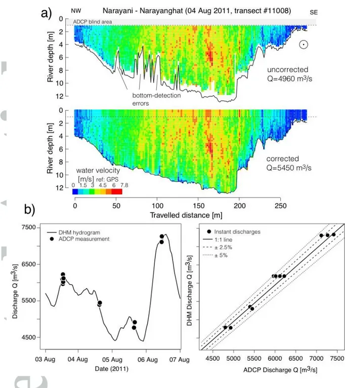
Although ADCP measurement is a relatively standard technique, operating on the Narayani River was challenging for several reasons. Hence, the ADCP current velocity dataset acquired during the 2011 monsoon showed inconsistencies due to technical limits during high flow conditions. High current velocities, as high as 7 m/s (32 km/h), made it difficult to maintain the boat trajectory perpendicular to the flow. Despite employing a narrow-solid-angle echo sounder to detect the channel bottom, we recorded important inconsistencies marked by unrealistic spikes in the topographic profile. We suspect areas of high turbulence and vertical eddies, highly concentrated sediment plumes near the river bottom, or large drifting objects (e.g., logs) to have induced these bottom-detection anomalies (Fig. 2a, top). Data were exported with the WinRiver software but discharges were underestimated due to the anomalies. Hence, the data were numerically post-treated with R software. To derive water velocities over the whole section and compute water discharge, we corrected the bottom-detection errors to a realistic topography and filled the missing velocity data by fitting a law of the wall to the top ~1.2-m layer blind to the transducer and the 0.5-m-thick bottom layer in the ADCP raw image (Fig. 2a, see supporting Text S6 for correction details). Double integration of the corrected velocity section over the local water depth and across the section provides the discharge value Q.
After correction, ADCP-derived discharges are in good agreement with discharges reported by the DHM station 3 km upstream (Fig. 2b). DHM discharges are converted from hourly water level reports using a rating curve. Although discharges varied from 4,500 to 7,500 m3/s during our 4-day campaign, the twelve ADCP discharge values differ by <5% from the DHM values.
ADCP data were acquired during depth sampling in the beginning of August 2011, when the monsoon is well established and the river is continuously at a high stage. Although our direct
observations missed the most extreme floods (Q > 10,000 m3/s), they document Narayani River discharges within the upper 25% of the DHM daily record since 1962 (supporting Figure S2). We thus consider that our observations well document sediment transport during moderate floods, which are more frequent than larger floods and cumulatively transport most of the annual sediment export (Wolman & Miller, 1960; Andermann et al., 2012a).
4.1.2. Flow separation, snow/ice melt, and the hydroclimatic record
During the monsoon period, relating climatic variables to the evolution of sediment fluxes and their origins requires rainfall and temperature chronicles over the entire watershed. Eighty DHM weather stations document daily average precipitation in the Narayani basin (supporting Figure S4), but they are heterogeneously distributed over the watershed with more stations along the Lesser Himalaya and along valley thalwegs. This over-representation of weather stations along valley bottoms compared to ridges and crests was identified as a possible source of bias by (Burbank et al., 2003).
To circumvent this potential bias, we exploit the fact that, in most flow separation models, river hydrographs can be separated into two main components: runoff and baseflow. The baseflow component Qb represents the contribution from groundwater reservoirs that slowly responds to rainfall events, and the direct runoff or storm runoff component Qd represents the sum of infiltration and saturation excess overland flow and is characterized by short response and transfer times after rainfall events. In this region, (Andermann et al., 2012b) demonstrated that direct runoff represents a minor part of the river discharge during the monsoon period (~25%) although it exerts a major control on sediment fluxes exported from the mountain basins (Andermann et al., 2012a). We used flow separation to assess Andermann et al., (2012a)’s conclusions and isolated direct runoff for the year 2010. Furthermore, we estimated snow/ice melt to determine the contribution to runoff from high altitude areas, and hence the amount of sediment potentially coming from glacial erosion. We then compared these fluxes with geochemical tracers to decipher the erosion processes involved.
Many digital filters have been proposed to separate the river hydrograph components (e.g., (Arnold et al., 1995; TG Chapman et al., 1996; Arnold & Allen, 1999; Chapman, 1999; Wittenberg & Sivapalan, 1999; Furey & Gupta, 2001), but those developed by (Eckhardt, 2005, 2008) were efficiently applied to natural basins (Andermann et al., 2012a; Tolorza et al., 2014; Struck et al., 2015). More specifically in Nepal, Andermann et al. (2012b) used generic digital filters based on daily discharges adapted from (Eckhardt, 2005), setting the
recession constant a to 0.98 and the ratio of annual baseflow to annual streamflow BFImax to
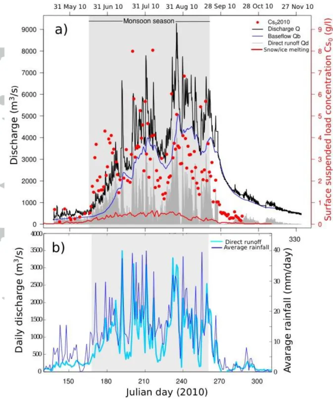
0.8 for all studied rivers. Here, to separate the 2010 Narayani hydrograph, we used the same digital filter (Fig. 3a), but set BFImax to 0.75 to improve hydrograph fitting. The recession
phase of the hydrograph during the postmonsoon period (beginning on Julian day 266 in 2010) slightly departs from an exponential curve: we accounted for this difference by varying
a nonlinearly between 0.987 at low baseflow and 0.91 at the highest baseflow. We also
adapted (Eckhardt, 2008)’s filter to the hourly discharge dataset by replacing the daily coefficient a by its hourly counterpart a1/24.
Integration of the 2010 daily discharge dataset provides annual Narayani discharge Qtotal =
48.1 km3/yr, annual direct runoff Qdtotal = 11.5 km3/yr (~24% of Qtotal), and annual baseflow
Qbtotal = 36.6 km3/yr (76% of Qtotal, coherent with BFImax set at 0.75). These figures are in
close agreement with previously reported values (Andermann et al., 2012b).
The direct runoff component closely follows the daily precipitation in the Narayani basin from early July until the end of the monsoon (Fig. 3b). During the premonsoon period in May and early June (Julian days 100–165), the discrepancy observed between rainfall and direct runoff indicates that a significant amount of water does not readily reach the streamflow. Several explanations likely contribute: 1) a certain amount of water is lost to evaporation because evapotranspiration is at its maximum during late spring (Bookhagen & Burbank, 2010; Andermann et al., 2012b); 2) a part of the precipitation may fall as snow, delaying the direct runoff response to rainfall; and 3) a certain amount of runoff infiltrates the ground surface as hypodermic flow to increase soil moisture when deeper water enters an aquifer as groundwater (Andermann et al., 2012b).
Finally, it has to be noted that the calculations described above cannot separate the rain and ice/snow melt flow components. If we assume that a major fraction of glacial meltwater is efficiently channelized and rapidly joins the river network, ice melt should contribute to the direct runoff rather than the groundwater component. Conversely, melting of the snow pack during the spring will rather infiltrate the ground and join the groundwater component. Hydrological modeling in the Dudh Kosi basin in Eastern Nepal (Nepal et al., 2014) suggests roughly equal partitioning between snow and ice melting in the hydrologic budget of that basin. For 2010, based on the DHM daily temperature records, the surface extent of glaciers (GLIMS Glacier Database) and SRTM topographic data, and based on a positive degree day model (PDD value or melt factor of 7 mm/°C/day for clean ice/snow and 4 mm/°C/day for debris covered ice below 5,000–5,200 m; (Kayastha et al., 2000; Wagnon et al., 2007 ;
Racoviteanu et al., 2013)), we estimate the total snow/ice-melting contribution to be ~8% of the annual Narayani discharge, with a peak contribution to the daily discharge of <10% during July (Fig. 3). Given this limited contribution, including snow/ice melt marginally modifies our flow separation data during the monsoon period (supporting Text S10).
4.2 Suspended load and sediment fluxes
4.2.1. Daily surface concentrations
Our suspended load concentration at the surface Cs0 data is in overall good agreement with
DHM measurements (supporting Figure S5). Except for the recession period at the end of September during which our data are systematically higher than the DHM data, more than two thirds of the datasets differ by less than 50%. More importantly, the slope of the correlation between the two datasets is very close to one (1.02, or 1.18 excluding the two main outliers). This suggests that lateral turbulent mixing of surface sediments between the central part of the channel and the riverbanks is relatively efficient, leading to a roughly uniform concentration increase with depth across the river section. Although the DHM sampling point is on the left bank of the Narayani only 1.8 km downstream from the confluence of the Kali Gandaki and Trisuli Rivers, the DHM record does not seem to be substantially impacted by incomplete mixing between the suspended load of these two contributing rivers, and is a priori representative of the entire Narayani watershed.
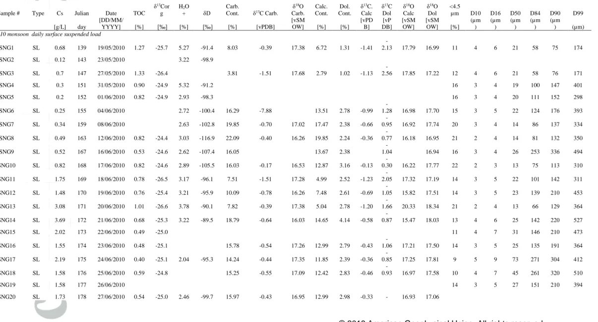
Temporal variations of Cs0 (Table 1) during the 2010 monsoon roughly follow the river
hydrograph (Fig. 3). Cs0 is quite low during the premonsoon period, and starts exceeding 1
g/L when monsoonal precipitation begins in mid-June (Julian day 166) and the Narayani discharges rises above 1,000 m3/s. During the monsoon, i.e., until mid-September (~Julian
day 260), Cs0 variations roughly mimic discharge variations, including reduced flow periods
around mid-August (Julian days 217–230) and flood peaks of intense direct runoff events corresponding to Cs0 increases above 4–8 g/L. When precipitation stops in the postmonsoon
period, Cs0 rapidly drops to values <0.5 g/L, whereas direct runoff decreases slowly.
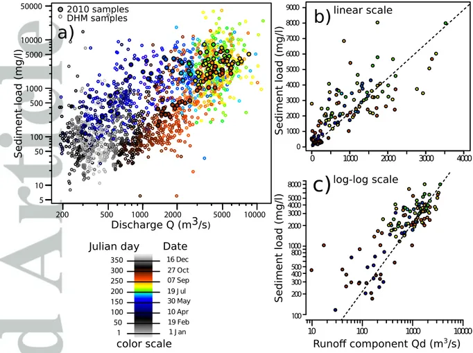
Throughout the course of one year, suspended sediment Cs0 plotted against daily Narayani
discharge Q displays a clockwise hysteresis loop (Fig. 4a) interpreted as dilution by the increased contribution of groundwaters discharging into the streamflow at the climax and until the end of the monsoon (Andermann et al., 2012a; Tolorza et al., 2014). In 2010, this
period corresponded to late July to mid-September (Julian days 210–260) during which Qb was above 2,500 m3/s and represented almost all of the total Narayani discharge.
As proposed by (Andermann et al., 2012a) for several Himalayan rivers, the sediment load-discharge hysteresis is reduced or eliminated when the groundwater load-discharge component is removed from the total discharge, i.e., when Cs0 is displayed versus the direct runoff
component Qd. During the 2010 monsoon, our data
confirm their observation and display a rough positive relationship between Cs0 and Qd (Fig.
4b, c).
4.2.2. Suspended sediment distribution in the water column
Vertical sampling profiles obtained in 2005, 2007, and 2011 display Cs0 values
ranging from 1.4 to 4 g/L, with an average of 2.44 g/L (Table 1, Fig. 5).
Sediment concentration increases with depth in the 2011 profiles whereas the 2007
concentration profile is almost uniform, although it was sampled at a lower discharge (~3,000 m3/s).
Due to high flow conditions in 2011, dredging bedload samples would have required a much heavier version (Edwards & Glysson, 1999) of our original Helley Smith bedload sampler. Nonetheless, former depth profiles sampled in 2005 and 2007 (PB and LO, respectively) with a bottom triple-sampler provide constraints on the bottom suspended and bedload concentrations. As expected, bottom samples PB54 and LO758C show very high concentrations of 10.24 and 30.90 g/L, respectively, illustrating the sharp concentration increase at the transition-layer between suspension and bedload, whereas the deepest concentration measured in 2011 was 6.67 g/L. Successful river bed dredging in 2007 returned only gravels and pebbles, suggesting that sand was entirely in suspension. However, the available data are too scarce to unravel the exact bedload concentration.
Narayani River suspended sediments are principally composed of fine to medium sand (following the Wentworth grain size chart), and mainly display unimodal grain size distributions (supporting Fig. S9). The 2011 depth profiles display a clear downward coarsening as illustrated by the constant increase with depth of the size of the 90th percentile of the grain size distribution D90 (Fig. 5), as expected from Rouse and other suspension theories (Rouse & others, 1950; Garcia, 2008). Surprisingly, i.e., in contrast with these
suspension theories, we do not observe significant variations of the grain size gradient with depth when discharge varies between 3,000 and 7,000 m3/s.
We explored lateral variability of Cs(z) using two depth profiles sampled in sequence between 1000 and 1130 local time on 7 August 2011 with almost equal hydrological conditions. The first profile (samples #CA11125–CA11128) was realized on the axis of the river and the “off-axis” profile (samples #CA11129–CA11131) was realized at ¼ of the channel width from the right bank. The on-axis and off-axis Cs(z) profiles are the same, suggesting efficient lateral diffusion of turbulence and of the sediment load over the river section. This result is coherent with the observed similarity between the surface concentrations measured at the middle of the river (Narayanghat bridge) and along the riverbank (DHM gauging station; see previous section).
The exact reasons why the concentration and grain size data display a roughly uniform gradient with depth and seem poorly dependent on the discharge are beyond the scope of this study. We rather build on the observed linear increase of concentration with depth, valid at least for discharge values between 3,000 and 7,000 m3/s (i.e., during 70% of the monsoon period), to perform depth integration in sediment flux calculations. For that, we approximate the suspended load concentration at depth z and time t, Cs(z,t), by the linear relation:
Cs(z,t) = (1+ K × z)×Cs(0,t), (1)
where Cs(0,t) is the surface concentration and K = 0.12 ± 0.04 m-1 is the average slope of the
Cs profiles as estimated from the depth sampling profiles. Based on the absence of significant
lateral variability in the concentration profiles, we additionally assume that this relation holds over the entire river section, such that the sediment flux through the river section can be derived, by first approximation, from a single Cs0 value.
4.2.3. Sediment flux calculation
Calculating the total suspended load flux of the Narayani River during the monsoon season requires a triple integration over the water depth, channel width, and over time. To proceed, we first modeled the topography of the river channel by considering the channel profiles sounded during ADCP cross-sections #11006, 11008, 12000, and 12001, which encompass the sediment depth sampling locations (Figs. 1 and S1). We orthogonally projected the ADCP bottom channel topography with respect to the river axis, and averaged all transects into a Synthetic transversal River Section (SRS; supporting Fig. S7A). We derived a rating curve
for this mean transversal section by computing water discharge Q through that section for any local water height H between 0 and 14 m.
To estimate the water velocity distribution in the section, we hypothesize that the law of the wall applied to the whole water column (details in Appendix A), so that:
Q(H ) = u( x,z,H )dx dz 0 zb( x )
ò
Xlb( H ) Xrb( H )ò
@ g Se(H ) zB(x, H ) k ln 30(zB(x, H ) - z) ks æ è ç ö ø ÷dx dz 0 zB( x )ò
Xlb( H ) Xrb(H )ò
(2)where u(x,z,H) is the water velocity at lateral position x, depth z, and height H, Xlb and Xrb
represent the left and right bank abscissa, Se(H) the energy slope for water elevation H, g the
gravity constant, κ the Von Karman constant taken at 0.41, zB(x,H) the local bottom depth
counted from the water surface, and ks the effective roughness height here defined by 3 × D50
= 0.22 m from the pebble median size measured on local Narayani gravel bars (supplementary Table S2; (Mezaki & Yabiku, 1984; Attal & Lavé, 2006; Dingle et al., 2016)). In equation (2), Se(H), is assumed to be constant around 0.05% (see justification and
sensitivity test in supporting information S7).
To compute the total suspended load flux, we rely on the assumptions that the surface concentration is uniform at any given time, and that the depth profile Cs(z) follows a linear trend of constant slope, as described in the previous section. The instantaneous sediment flux can thus be simplified, according to equations (1) and (2), into:
) ( ) ( ) , ( 0 )) ( , , ( 0 ) ( ) ( ) , ( 0 )) ( , , ( ( ) () . ). , ( ) ( t X t X x t z t Q z x s t X t X x t z t Q z x s s rb lb b rb lb b dxdz u z K t Q t C dxdz u t z C t Q . (3)This double integration of z and u on space variables was numerically performed, but can be approximated for rapid use by the closely fitting relationship that we homogeneised in dimension: Qs(t) = Cs0(t)×Q(t)×(1+ K*×exp(-1.9561+ 0.5517×log(Q(t) Q* ) - 0.0185× log( Q(t) Q* ) 2 ). where, K* = 0.12 dimentionless and Q* = 1 m3/s.
Finally, to realize time integration, we can follow distinct pathways. DHM discharge measurements provide an hourly record, whereas our suspended load sampling was performed on a daily basis. To compute sediment flux over the monsoon period or an entire year, we assume that the hydrology of the Narayani River is slowly varying and that the concentration measured each day at 0800 local time is representative of the mean concentration during that day. In this first case (case DMC), we simply assess the mean daily
discharge from the daily value measured at the DHM gauging station, derive the water height at the SRS from the synthetic rating curve, insert the measured surface concentration into equation (3), interpolate values between biweekly measurements during the monsoon period, and sum the daily mean sediment fluxes over the entire year.
In a second approach, we recognize that the large daily variations observed in our Cs(t) data might be related to higher frequency variations during a day. In that case, we need to define an empirical sediment rating curve. Classically, the suspended load concentration is linked to water discharge through a power law, which holds when a river system is transport limited, i.e., when available sediment on the channel bottom is unlimited and only hydrodynamic conditions determine a river’s sediment carrying capacity. However, in active mountain ranges, rivers are mostly supply-limited (Fuller et al., 2003; Andermann et al., 2012a), and a plot of discharge against concentration displays poor correlation or non-linear behavior, including hysteresis (Fig. 4a).
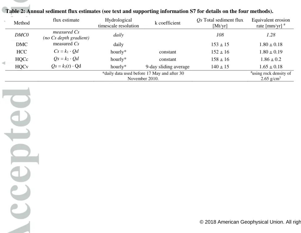
To document sediment flux, we chose to explore three hypotheses or relations in estimating the hourly values of Cs(t) ( Table 2 and supporting information S7) .
One of the aims of this study was to improve former sediment flux estimates for the Narayani River, in particular by integrating Cs along the water column based on depth sampling
measurements. Accounting for increasing concentration with depth, i.e., the second integral member in equation (3), increased the calculated sediment flux by ~45% compared to the constant concentration profile case (case DMC0 in Table 2). In contrast, the time integration scheme has much less impact on the results: the four calculations using different time-step integrations or concentration estimates (cases DMC and the three hourly-based calculations in supporting information S7) lead to very similar estimates ranging between 140 ± 14 and 158 ± 15 Mt/yr (Table 2). We thus estimate the annual suspended load flux in 2010 to be 151 ± 20 Mt/yr.
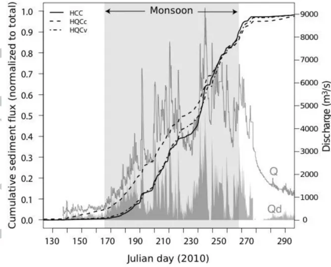
To document the timing of sediment delivery, cumulative fluxes were calculated over the year and are presented in Figure 6 normalized to their respective total budgets and compared to the discharge and direct runoff chronicles. Clear increases in sediment flux are observed during periods of sustained rainfall and intense runoff, regardless of the sediment flux calculation. Even if the rainy episode during Julian days 230–238 yielded 20–25% of the annual sediment budget, most of the suspended sediment volume exported by the Narayani River results from the cumulative effect over the whole monsoon rather than from a few
events. This moderate sensitivity of the total flux to extreme events (and conversely to the dominant role of cumulative average monsoonal floods) explains a priori that the four explored methods for calculating sediment flux converge toward relatively similar values.
4.2.4. Average sediment flux over recent decades
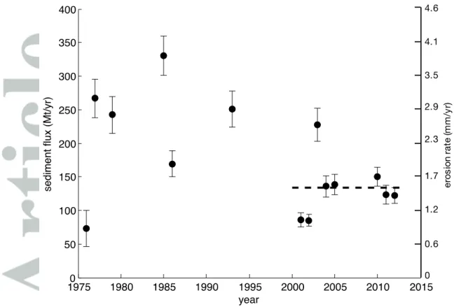
In active mountain ranges, landslides are considered as the major hillslope erosion process and thus the major source of river sediments. Because of the stochastic nature of landslides and mass wasting, and given that the erosional budget may be dominated by rare and very large landslides (Hovius et al., 1997), we consider that the annual sediment flux should also be stochastic by nature (Fuller et al., 2003) and should vary interannually. Deriving a mean erosional flux for the Narayani basin therefore requires averaging the sediment flux over several years or decades. Accounting for increasing sediment concentration with depth using equation (3), we derived sediment flux by applying the aforementioned DMC approach to the 14 noncontiguous years of available DHM sediment records and corresponding daily discharge records. We also used the HCC approach (Table 2) on a daily basis to derive direct runoff components to complement numerous gaps in the database.
The results display two basic domains: before 2000, annual sediment fluxes (Fig. 7) varied greatly, with annual fluxes up to 150% higher than our reference year 2010 and large interannual variations. In contrast, since 2000, the annual fluxes were less scattered. We partly ascribe the higher values pre-2000 to the use of integrative USGS sampling bottles during the early recording years, which implies that the concentration increase with depth was already accounted for in the raw data. We do not know, however, when the protocol changed to surface sampling. In the absence of further information, we limited our averaging period for the mean flux calculation to the years after 2000. During that period, the average suspended load flux was 135 ± 15 Mt/yr, slightly lower than in 2010.
4.3. Seasonal evolution of the suspended load characteristics
The sediment flux exported by the Narayani provides essential data on the amplitude of denudation in the basin, but does not provide information on the geographical origins or erosional processes that feed the fluvial network. In this section, we assess the monsoonal evolution of each erosional process contributing to the sediment yield with different tracers: grain size evolution is used as an indicator of mass wasting inputs into the network, carbonate
content and D/H composition are used to trace contributions from northern/glaciated versus southern/unglaciated basins, and TOC is used as an indicator of soil erosion.
4.3.1. Grain size evolution: sediment inputs from mass wasting
Generally, in-channel processes lead to grain size fining during transport, either by selective transport (e.g., Paola et al., 1992)) or pebble abrasion (e.g., Attal & Lavé, 2009). Nevertheless, sediment coarsening along a river channel has been observed in mountain ranges as a result of variations in hillslope sediment supply (e.g., Brummer & Montgomery, 2003; Attal & Lavé, 2006; Struck et al., 2015). In this study, we analyze grain size evolution during an entire year at the basin outlet to infer the evolution of the sediment supply in response to climatic forcing.
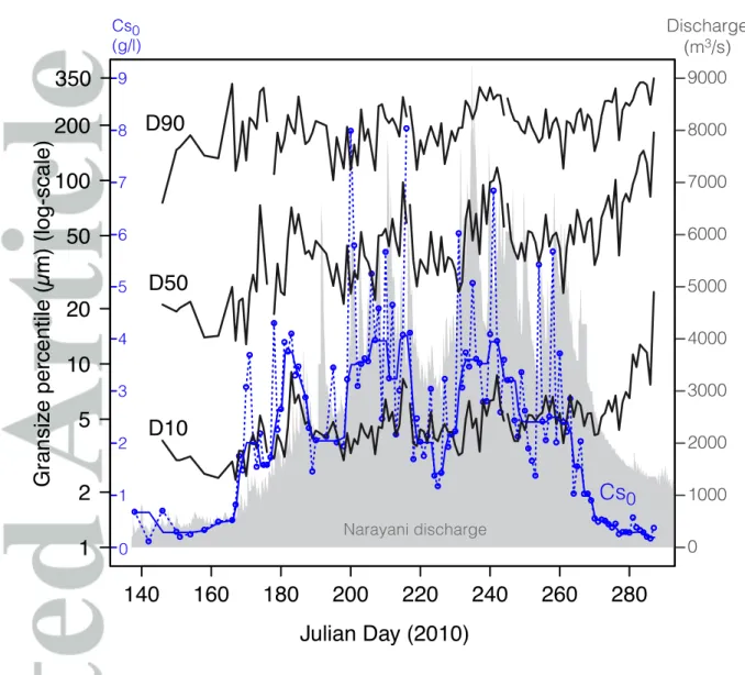
Figure 8 presents the evolution of the suspended sediment grain size distribution synthesized by D10, D50, and D90, the surface sediment concentration Cs0, and river discharge at the
Narayani basin outlet during the 2010 monsoon (see also supporting Figure S8 for the full cumulative distribution curves and Figure S9 for the time-series of the sediment fraction finer than 4.5 µm).
During the three monsoonal months, sediment sizes D10, D50, and D90 roughly follow fluctuations of Cs0 with high-frequency variations occurring with amplitude of a factor of 2–
3. The three most prominent peaks on Julian days 182, 215, and 242 are coincident with peak
Cs0 values of 4–8 g/L, suggesting that coarser-sediment events are related to pulses of
sediment supply triggered by intense rainfall events (see sections 4.1.2 and 4.2.1). We interpret these pulses as resulting from the triggering and functioning of mass wasting processes and landslides, providing an important supply of coarser sediments (Attal & Lavé, 2006; Struck et al., 2015) during periods of continuous rainfall. Despite large daily variations, the suspended sediment grain size generally increases throughout the five months investigated: specifically, D10, D50, and D90 roughly double during the three monsoonal months, respectively starting at 3, 20, and 100 μm on Julian day 165 and reaching 6, 50, and 200 μm on Julian day 258. We also consider this trend to represent a progressive overwhelming of the sediment supply by coarse mass-wasting-derived materials.
During about three weeks after the monsoonal months (late September to mid-October; Julian days 270–290), D10, D50, and D90 abruptly coarsen to 20, 200, and 350 μm, respectively. Since mass wasting should have stopped providing sediments to the channels when rainstorms ceased (~Julian day 270), the drainage system acts as a semi-closed system,
essentially carrying only the available sediments that accumulated during the monsoon. In contrast to the monsoon, we interpret this postmonsoon coarsening to result from transport in channels, which induces a progressive flush of the more easily transported fine sediments and a delay in the arrival of slower coarser sediments.
4.3.2. Evolution of D and carbonate content: N-S source tracers
Because the Narayani basin presents contrasted lithologies from north to south, the suspended sediment composition can be used to discriminate the N-S provenance of sediments exported at the basin outlet. Carbonates mostly outcrop in the western and northern part of the basin (Dhaulagiri and Annapurna Massifs) in the TSS rather than in the crystalline High Himalayan range (Colchen et al., 1986). The tributaries draining the TSS display a large range of carbonate content, up to 65%. Sands sampled along the banks of the upper Marsyandi tributaries have intermediate carbonate contents from 25 to 30% (Fig. 10 and supporting Table S) whereas suspended loads sampled in rivers draining mostly TSS units present slightly higher proportions of 40 ± 7%. Dudh khola sediments display exceptionally low carbonate contents because its drainage system is dominated by leucogranites. In the south flank, Marsyandi tributaries carry much lower proportions of carbonates, between 0 and 8%, which mostly originate from the upper LH units. In the East, the Trisuli river and its tributaries carry minute amount of carbonates as TSS is restricted to the Bothe Kosi far to the north of its basin (Galy et al. 1999). Narayani River sediments have variable carbonate contents from 5 to 25% (Fig. 9a and Table 1), with typical values between 10 and 20%. The average content (sediment-flux-weighted average) of the material delivered by the Narayani River from May to mid-October is 14.8%, implying that at least 30% of the Narayani suspended load derives from the TSS (~40% carbonates) and 70% from other geological units (0–8% carbonates).
The hydrogen isotopic composition of hydrated silicates reflects both the original bedrock composition (i.e., metamorphic water mostly contained in micas and chlorites, with δD values around –90‰ (France-Lanord & Sheppard, 1988) and water incorporated into secondary minerals as hydroxyl during weathering. The isotopic composition of the latter depends on that of local meteoric water, which in the Himalaya is dependent on the combined effects of distillation linked to orographic precipitation and elevation (Garzione et al., 2008). Consequently, river sediments derived from the northern watersheds and glaciated
environments display low δD values around –160 to –110‰, such as sediments of the upper Marsyandi, Naur, Dudh, Dona rivers, or Langtang area in the eastern part of the Narayani watershed (see location in Fig. 1), particularly the fine sediments (glacier flour) collected at the outlet of the pro-glacial streams in front of Dudh and Langtang glaciers (Fig. 10). In contrast, river sediments from lower elevations along the southern flank of the Himalaya or from tributaries draining elevated TSS lithologies along nonglaciated basins (Sabche, Bratang or Ghatte rivers in the Upper Marsyandi), display higher δD values between –100 and –80‰ (Khudi, Chepe, Darondi, Dordi, Paudi, Ngadi khola on Fig. 10), similar to pristine bedrock values. These results suggest that lower δD values are preferentially indicative of sediments issued from weathering associated with glacial erosion.
Hydrated silicates in Narayani River sediments span a wide range of δD values over the monsoon period, from –87 to –117‰ (Fig. 9), with high-frequency variations but no seasonal trend. Most days (72.5%) present a δD value greater than –100‰, consistent with a dominant signature of unweathered bedrock or weathered material issued from the southern Himalayan flank, whereas some days display isotopic compositions that require a significant or even dominant contribution of sediments issued from the upper glaciated catchments. When compared to the contribution of ice melting to the Narayani River discharge, the glacial sediment contribution is apparent during the premonsoon and early monsoon periods (Fig. 11, supporting Text S10).
Daily Narayani suspended sediment samples appear to cover almost the full spectrum of carbonate and δD compositions documented within the basin from north to south, and show a rough anti-correlation (Fig. 10). It is consistent with the fact that a large fraction of the glaciers feeding the Narayani River, mostly in the Annapurna and Dhaulagiri basins, are eroding TSS carbonate-rich formations. During the premonsoon and early monsoon periods (before Julian day 180), the δD data appear to follow the relative contribution of ice melting to the Narayani discharge, with the most negative value recorded in mid-June (Julian day 163) when ice melting had reached a maximum contribution of ~50% (Figs. 3 and 11). This overall agreement during a month-long period is only interrupted by the first major monsoonal rainfall event on Julian day 171, which produced a fivefold increase of the suspended load concentration (Fig. 3b) and probably diluted the glacial sediment signal during a couple of days. In contrast, the relative contribution of ice melting was lower than 10% during the monsoon, and no clear relation was found to explain the observed δD
variations. This lack of correlation probably reflects that glacial erosion and erosion of carbonates can be locally uncorrelated: in the eastern part of the Narayani watershed or in the Manaslu area, glaciers primarily erode granitic or gneissic massifs, whereas a large portion of the carbonate-rich TSS lithologies outcrop along unglaciated hillslopes. Both carbonate content and δD values show similar high-frequency variations, indicating that the origin of the sediments, whether related to distinct geographic sources or an erosion process, can vary quite abruptly throughout the season and rapidly respond to local events and meteorological conditions.
4.3.3. Evolution of TOC: superficial soil erosion
TOC in the top horizons of soil profiles in the Himalaya reach very high values from a few to more than 10 wt% (e.g., Lorphelin, 1985; Right & Lorphelin, 1986; Shrestha et al., 2004; Bäumler et al., 2005; Caspari et al., 2006; Dorji et al., 2009). In this study, we use TOC as an indicator of the proportion of soil-derived material in the Narayani suspended sediment. Daily measurements of TOC in Narayani suspended sediments during 2010 varied between 0.2 and 1.3 wt%. During the premonsoon period TOC are high, around 1 wt%, and drop to 0.2–0.5 wt% after the first heavy rainfall and discharge event on Julian day 171 (Fig. 9b) and through the postmonsoon season. Organic carbon was reported to be preferentially associated with fine particles in Himalaya-derived sediments (Galy et al., 2008). During the monsoon, TOC in the Narayani suspended load follow the grain size-controlled relation established for large Himalayan rivers by Galy et al. (2008), despite large scatter (supporting Fig. S11). In contrast, during the premonsoon period, TOC values are well above the Himalayan rivers trend while fine sediment proportions are important (supporting Fig. S11). Therefore, grain size sorting in the water column cannot account for such high TOC when discharge and sediment suspension are low. Although TOC is not a completely conservative tracer because it is affected by various processes during fluvial transport (e.g., Battin et al., 2008; Galy et al., 2008), high TOC in Narayani River sediments during the premonsoon period could reflect higher inputs from sources enriched in soil or organic matter (vegetal litter). During the monsoon, Narayani TOC values remain low in the 0.2 to 0.5 wt% range. This is above the range of bedrock (0.05 to 0.1 wt%, Galy et al. 2007) but much lower than soil derived material, which we interpret as evidence that the contribution of soil erosion is dwarfed by that of mass wasting.
5.1 Sediment flux calculation: depth sampling and general strategy
Previous estimates of the Narayani suspended load flux are 100 ± 50 Mt/yr (Sinha & Friend, 1994; Andermann et al., 2012a). Our estimates of 150 ± 20 Mt/yr for 2010 and 135 ± 15 Mt/yr during the previous decade based on DHM data are in the higher range of previous estimates because they account for vertical variations of concentration with depth, whereas we obtain a flux around 100 Mt/yr when this gradient is ignored (case DMC0, Table 2). Thus, even when the Narayani River is highly turbulent during monsoonal floods, vertical sorting must be integrated into the sediment flux; otherwise the Narayani sediment flux can be underestimated by up to 50%. Our approach to integrating the concentration over depth is simplified and based on measurements operated during only a few days. To perform depth integration on a more physical basis, a complementary study would be necessary to document the concentration gradient during low to intermediate (<3,000 m3/s) and very high flows (>7,000 m3/s). However, as the range of flow conditions during our sampling campaigns encompasses >85% of the exported sediment flux (due to reduced load flux at low flow and the rare occurrence of the highest flow conditions), we do not expect major bias in our estimates. Furthermore, the depth-integration term in equation (3) depends only on the water discharge and can be applied to any future (or past) record of surface suspended load concentration without depth sampling.
However, given the highly variable rating curves obtained from DHM data between 1975 and 2012 (supporting Fig. S12) and the geomorphologic considerations previously mentioned, we suggest that deriving a unique and constant sediment rating curve in a supply-limited system is probably not relevant (see also section 5.4). Even if sediment production and mobilization on hillslopes seem roughly correlated to runoff flow, by assuming the robust relation between direct discharge and sediment flux (supporting Fig. S7C), the relation Qs = f2(Qd) can vary
amply through time. This is likely related to the stochastic behavior of very large contributing landslides, or the complex combined control of ground saturation and rainfall intensity in triggering landslides (Gabet et al., 2004b; see also section 5.3), implying that the dependency of sediment flux on direct discharge also varies through time. The 14 years of DHM sediment chronicles suggest that such variations need to be accounted for at least on an annual basis. The small clockwise hysteresis observed in the June 2010 sediment flux (supporting Fig. S7C) might suggest that such variations should be considered even on a monthly to weekly basis.