HAL Id: hal-02870639
https://hal.archives-ouvertes.fr/hal-02870639
Submitted on 16 Jun 2020
HAL is a multi-disciplinary open access
archive for the deposit and dissemination of
sci-entific research documents, whether they are
pub-lished or not. The documents may come from
teaching and research institutions in France or
abroad, or from public or private research centers.
L’archive ouverte pluridisciplinaire HAL, est
destinée au dépôt et à la diffusion de documents
scientifiques de niveau recherche, publiés ou non,
émanant des établissements d’enseignement et de
recherche français ou étrangers, des laboratoires
publics ou privés.
atmospheric global distribution of sea salt aerosol
Walter Guelle, Michael Schulz, Yves Balkanski, Frank Dentener
To cite this version:
Walter Guelle, Michael Schulz, Yves Balkanski, Frank Dentener. Influence of the source formulation on
modeling the atmospheric global distribution of sea salt aerosol. Journal of Geophysical Research:
At-mospheres, American Geophysical Union, 2001, 106 (D21), pp.27509-27524. �10.1029/2001JD900249�.
�hal-02870639�
Influence of the source formulation on modeling the
atmospheric global distribution of sea salt aerosol
Walter Guelle, Michael Schulz, and Yves Balkanski
Laboratoire des Sciences du Climat et de l’Environnement, Commissariat a` l’Energie Atomique– Centre National de la Recherche Scientifique, Gif-sur-Yvette, France
Frank Dentener
European Commission, Joint Research Center, Ispra, Italy
Abstract.
Three different sea salt generation functions are investigated for use in global
three-dimensional atmospheric models. Complementary observational data are used to
validate an annual simulation of the whole size range (film, jet, and spume droplet derived
particles). Aerosol concentrations are corrected for humidity growth and sampler inlet
characteristics. Data from the North American deposition network are corrected for
mineral dust to derive sea salt wet fluxes. We find that sea salt transport to inner
continental areas requires substantial mass in the jet droplet range, which is best
reproduced with the source of Monahan et al. [1986]. The results from this source
formulation also shows the best agreement with aerosol concentration seasonality and sea
salt size distributions below 4
m dry radius. Measured wind speed dependence of coarse
particle occurrence suggests that above 4
m the source from Smith and Harrison [1998] is
most appropriate. Such sea salt simulations are relevant for assessing heterogeneous
chemistry and radiative effects. Sea salt aerosol provides on an annual average, in marine
regions, an aggregate surface area equal to 1–10% of the area of the underlying Earth’s
surface. Together with mineral dust, sulfate, and carbonaceous aerosol the total aerosol
surface area globally amounts to 13% of that of the Earth’s surface. On the basis of
atmospheric column burdens, sea salt represents 21% of the total global aerosol surface
area. Equal partitioning of the aerosol surface area among the four components suggests
that one has to consider all of them if the global aerosol impact is to be fully determined.
1. Introduction
Sea salt aerosol produced by the action of wind at the ocean surface constitutes the most abundant aerosol component to-gether with mineral dust. Sea salt studies have addressed its impact on tropospheric chemistry, radiation balance, or air/sea exchange of matter and energy. Finlayson-Pitts [1983],
Finlay-son-Pitts et al. [1989], and Behnke et al. [1997] have shown that
the reaction of NO2and N2O5with NaCl aerosol in the marine
boundary (MBL) provides an effective initiation pathway for atomic chlorine. Sea salt is also responsible for a large fraction of the non–sea salt sulfate formation since it is an important sink for SO2in the MBL [Sievering et al., 1991, 1992; Chamei-des and Stelson, 1992; Gurciullo et al., 1999]. Furthermore, the
alkalinity of sea salt as cloud condensation nuclei affects aque-ous chemistry [van den Berg et al., 2000].
Murphy et al. [1998] and Quinn and Coffman [1999] have
shown that over wide oceanic areas, sea salt is the most effi-cient aerosol component to scatter solar radiation. Haywood et
al. [1999] invoked sea salt to explain the bias in solar
reflec-tion between a general circulareflec-tion model (GCM) and ERBE satellite. Submicrometer sea salt competes with sulfate to influence the number of cloud condensation nuclei (CCN)
and thus participates into the aerosol indirect effect [Latham and Smith, 1990; O’Dowd et al., 1999a, 1999b]. Finally, giant sea salt particles have been invoked in the transfer of heat and moisture between the ocean and the atmosphere [Andreas et al., 1995].
Global chemical models used to estimate the chemical and radiative impacts of sea salt have had simplified representation of the size spectrum. The representation of the aerosol size and of its distribution is key for such estimates derived from models. We study in this paper three different sea salt gener-ation functions that have been published and are widely used. We focus on their ability to reproduce accurately the whole sea salt size distribution.
These three generation functions of sea salt particles are
Monahan et al. [1986] (hereafter referred to as Monahan); Smith and Harrison [1998] (referred to as SmithHar); An-dreas [1998] (referred to as AnAn-dreas). Each one provided
the input for a yearly simulation in the global transport model. Results from the three simulations are compared to measurements over different parts of the sea salt size spec-trum. On the basis of the model/measurements comparison, we discuss which source function is most adequate to rep-resent sea salt mass distribution and deposition on large scales. The physical characteristics of the global sea salt aerosol distribution (mass burden, surface area, number, etc.) are also compared to sulfate, carbonaceous and min-eral aerosol distributions.
Copyright 2001 by the American Geophysical Union. Paper number 2001JD900249.
0148-0227/01/2001JD900249$09.00
2. Previous Global Modeling Studies of Sea Salt
To our knowledge, sea salt atmospheric cycle has been in-cluded into only four global models. Genthon [1992] and Tegen
et al. [1997] used a source formulation which fixes the surface
level concentration [Erickson et al., 1986] as a function of wind speed, instead of estimating a flux at the air-sea interface. This formulation uses a single set of coefficients (slope and inter-cept), deduced from observations of Lovett [1978], to deduce the surface layer sea salt mass concentration from the 10-m wind speed. The intercomparison of similar relationships by various authors [Fitzgerald, 1991; Gong et al., 1997a] showed significant differences between derived sets of coefficients. The different measurement techniques permit derivation of rela-tionships over limited parts of the size spectrum. Any extension to other parts might be hazardous.
The most recent global simulation of sea salt aerosol uses the Canadian general circulation model (GCM) [Gong et al., 1997a, 1997b] which Erickson et al. [1999] used to derive a reactive chlorine emission inventory. The source flux follows Monahan using his formulation for a dry radius of particles up to 8m. The results of the simulation are compared against monthly and yearly averaged sea salt concentrations observed in surface air at five coastal stations. Seasonal variability con-tributes an important part to the overall variability of the atmospheric sea salt loading.
3. Model Description
3.1. Transport Model and Aerosol Physics
We use the TM3 global atmospheric tracer transport model. This model divides the vertical dimension into 19 hybrid levels, whereas the TM2 model [Heimann, 1995] had only 9 isobaric levels. The horizontal resolution is 5⬚ longitude ⫻ 3.75⬚ lati-tude, and this version has been previously used by Houweling et
al. [1998] and by Lelieveld and Dentener [2000] for gas
chem-istry studies, as well as by Dentener et al. [1999] to study222Rn
transport. The TM3 version took part into a model intercom-parison of the transport of SF6 [Denning et al., 1999].
Six-hourly fields of temperature, humidity, clouds, and precipita-tion from the European Center for Medium-Range Weather Forecasting (ECMWF) are used as input to compute the mod-el’s dynamics, as well as the aerosol source and sinks.
The aerosol physics was previously developed in a module to study 210Pb [Guelle et al., 1998a, 1998b] and mineral dust
[Schulz et al., 1998; Guelle et al., 2000]. Aerosol sedimentation and below cloud scavenging are both treated as size-dependent processes. Other aerosol sinks include turbulent dry deposition and particle scavenging by convective and synoptic precipita-tion.
The radius and the density of sea salt particles are largely affected by its hygroscopicity. We accounted for their evolution in time as a function of relative humidity (RH) conditions. At each model time step, for every grid box and size bin, radius and density were computed as a function of the mean dry radius and ECMWF three-dimensional (3-D) fields of specific humidity and temperature [see Gerber, 1988]. We assumed the particles to be spherical and to have the pure NaCl ionic composition.
3.2. Sea Salt Generation Functions
Two main mechanisms are thought to control sea salt for-mation: bubble bursting and tearing of wave crests by wind.
Bubble bursting is believed to produce the film and jet drop-lets, and tearing of wave crests by wind forms the larger spume drops. Particles with rdryⱕ 0.5m are commonly referred to
as film drop range, particles with dry radii between 0.5 and 4 m as jet drop range, and particles with rdryⱖ 4m as spume
drop range; rdrycorresponds to the radius of the particle at 0%
RH. Hereinafter we will often refer to small particles to in-clude film drop and jet drop range (rdry ⱕ 4m) and large
particles as particles formed in the spume drop range. The different formulations of the sea salt aerosol generation function are presented in the review by Andreas [1998]. Surface fluxes differ by several orders of magnitude between two dif-ferent formulations. One goal in this paper is to propose one formulation based upon previous work to represent particles with dry radii from 0.03 to ⬃64m. The equations from the three formulations that we focus on have been included in Appendix A.
The first formulation, from Monahan, follows Gong et al. [1997a]. We chose to use the formulation up to a dry radius of 8m and in a later stage of this study up to 4 m, since it is thought to overestimate the production of very large sea salt particles [Andreas et al., 1995]. Andreas et al. [1995] pointed out that Monahan’s formulation could well describe the produc-tion of particles below rdry ⫽ 0.5m, and it was altogether
evaluated to give satisfactory results in a GCM (S. L. Gong, personal communication, 1999).
The second formulation is presented by Smith et al. [1993], with updated parameters from Smith and Harrison [1998]. Al-though limited to aerosol with radius larger than 1m at 80% RH (r80) (thus rdryof⬃0.5m), this formulation was derived
directly from measurements of very large marine aerosols and may be of special value for the large particle size fraction. The third and most recent formulation, from Andreas [1998], cov-ered the whole size spectrum of sea salt aerosol, accounting for all the previous studies. The production of large sea salt par-ticles via spume formation (discussed therein in terms of wet radius r80) is based on an extrapolation of the data of Wu et al.
[1984] for very large particles (r80 ⬎ 10 m). For smaller
particles (r80ⱕ 10 m), Andreas applied a factor 3.5 to the
formulation from Smith et al. [1993] in order to adjust it to the volume flux of Monahan for the size range 2m ⱕ r80ⱕ 7.3
m.
Figure 1 presents the sea salt mass production as a function of the dry radius for the three formulations and for four dif-ferent 10 m above sea level (asl) wind speeds. We insist upon the fact that the amount of water associated to sea salt can be very significant (rdry ⬇ 0.5r80). For illustration purposes, in
Figure 1 we show that sea salt generation functions with Smith-Har and Andreas produce a lot fewer particles below rdry⫽ 0.5
m than Monahan’s. For very large particles (4 m ⱕ rdryⱕ 64
m) the mass produced in the Andreas formulation is greater than that in the SmithHar formulation. For particles above 64 m the SmithHar formulation produces the highest mass flux. The three formulations have an interesting common inter-mediate size range, which we have chosen to range from rdry⫽
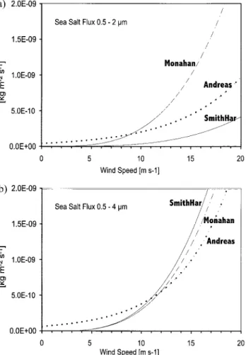
0.5 to 4m. This part of the size spectrum is significant both in terms of number, surface area, and volume [O’Dowd et al., 1997a]. Table 1 shows the model integration for a whole year. All three formulations show rather comparable results with regard to mass loads. Although similar at high wind speeds, the formulation of Andreas differs from SmithHar and Monahan by a factor of 5 at 5 m s⫺1(Figures 2a and 2b). However, the
due to the importance of high winds for the sea salt production for the smallest particles in this size range (see fluxes for rdry
0.5–2m in Figure 2a). Another noticeable difference between the three source functions is the varying wind dependency of the sea salt mass generated in this size range. Rather than retracing these differences in the equations of Appendix A, in sections 5 and 6 we discuss the manifestation of these differ-ences in the simulated atmospheric distributions.
Sea salt production is computed over the ocean every 6 hours using the ECMWF 10-m wind speed. No source flux is present in sea ice covered regions, identified from climatolog-ical monthly averaged data [Zwally et al., 1983]. The particles are generated with the three formulations previously discussed using a discrete bins scheme [Schulz et al., 1998] to represent
the size distribution. Class borders of each bin and the usage of the size information contained in these bins for the compari-sons made in this paper are given in Figure 3.
Finally, since we want to discuss the source formulations over the whole size spectrum, a composite source function is needed to account for the size interval over which these sources were formulated originally. For the size range up to 4 m and given the remarks above, the Monahan source formu-lation is used. Above the threshold rdry⫽ 4m we use either
the SmithHar formulation or the one from Andreas. The
Figure 1. Size-dependent sea salt mass flux simulated by the three formulations for four different wind speeds at 10 m.
Table 1. Mean Annual Global Loads of Sea Salt Mass, Aerosol Surface Area, and Particle Number With the Three Source Formulations
Dry Radius
rdry,m
Mass,
mg m⫺2 Surface Area,cm aer
2 m⫺2 Number,106m⫺2 Mass/Surface Area,mg cm aer ⫺2 Monahan ⱕ0.5a 1.0 59 50060 0.02 Monahan ⱖ0.5 to ⱕ4b 20.7 187 1245 0.11 SmithHar ⱖ0.5 to ⱕ4 8.8 48 89 0.18 Andreas ⱖ0.5 to ⱕ4 20.7 151 550 0.14 SmithHar ⱖ4c 16.5 22 3.5 0.76 Andreas ⱖ4 62.7 75 9.3 0.83
aVery small particle size (film drop range). bSmall particle size (jet drop range). cLarge particle size (spume drop range).
Figure 2. Integrated sea salt mass flux for the three source formulations as a function of wind speed integrated for the particle ranges. (a) 0.5–2m and (b) 0.5–4 m.
source flux is divided into seven bins for Monahan (0.031–4 m) and four bins for either SmithHar or Andreas (4–64 m) (see Figure 3).
4. Measurements Selected for Model Evaluation
Sea salt measurements are unevenly distributed over the globe. They are dense at northern midlatitude and not surpris-ingly sparse in less accessible remote regions. The selection of measurements toward an evaluation of the model requires selecting data representative of the scales resolved. The main selection criteria we applied were (1) can the measurements be related directly to sea salt aerosols, excluding other species such as organic and sulfate particles?; (2) are the observations representative enough at the scale of the model resolution (5⬚ ⫻ 3.75⬚)?; and (3) do the observations include information over a wide portion of the sea salt size spectrum?
We now discuss the measurements according to aerosol size. Where appropriate, we have also adapted the range of sizes from the model bins to correspond to the specific size range measured with the instrument. Table 2 summarizes the dis-cussed measurements.
4.1. Small Particles (Jet and Film Drop Range)
4.1.1. Aerosol measurements. The most common sea salt observations for a long time period are ground level measure-ments of Na⫹concentrations at coastal or island stations. The
sodium content of filter or impactor samples is generally de-termined by atomic emission or absorption spectrometry for Na⫹and by ion chromatography for Cl⫺. The sea salt
concen-tration is then derived considering a sodium amount of 30.8% in sea salt.
Ground level measurements of sodium are most represen-tative of aerosol with radii smaller than ⬃5 m in radius at ambient air conditions (sampling cutoff size corresponding to PM10). Collection efficiency can differ significantly from one instrument to another. Francois et al. [1995] intercompared five aerosol samplers in Mace Head (Ireland). He concluded that the major difference in measured sea salt concentrations was attributable to differences in the inlets. Howell et al. [1998] compared sea salt distributions measured by three widely used different types of cascade impactors. The comparison showed up to a factor of 4 difference between the Na⫹concentrations
determined with a Sierra impactor and a Berner impactor associated to differences in the instruments cutoff.
Unless otherwise indicated, the aerosol measurements that we used in this study have been carried out by D. L. Savoie and colleagues and have been reported by Gong et al. [1997b] and
Tegen et al. [1997]. Measurements at stations located in Asia
are properly referenced by Mukai and Suzuki [1996] and
Car-michael et al. [1996]. Measurements at Miami are reported by Prospero [1999].
Measurements of aerosol in the range below rdry⫽ 0.5m
have been motivated mainly by the interest that represent such abundant components as organic and sulfur. Unfortunately, the chemical speciation of sea salt is rarely conducted. Quinn
and Coffman [1999] have recently summarized NSS-SO42⫺and
sea salt mass size distributions obtained during several cam-paigns over the Pacific and Southern Oceans. They concluded that over these regions, sea salt can be a significant fraction of the this aerosol size fraction.
Sea salt particles with rdry⬍ 0.5m can be measured using
cascade impactors coupled to a chemical analysis using ion chromatography. Particle counters can be used in combination with a pretreatment of the aerosol (heating and evaporation of more volatile aerosol components). Higher temperatures in the evaporation step permit to identify directly the sea salt fraction [Smith and O’Dowd, 1996; O’Dowd et al., 1997a].
Our model evaluation will focus on data collected near the Faeroe Islands by O’Dowd and Smith [1993]. They derived the number concentration of sea salt as a function of 10-m wind speed for a dry radius of the particle included within 0.05 to 1.5 m. The sea salt mass size distributions that we compared are summarized by Quinn and Coffman [1999].
4.1.2. Wet deposition flux measurements. Sea salt wet deposition fluxes measured at continental sites away from the coast can be compared with the fluxes simulated by the model. Smaller particles contribute very little to the wet deposition of sea salt mass. However, the main advantage of these continen-tal observations is the absence of very large sea salt particles due to gravitational settling. A large data set of weekly wet deposition is available for the United States, which we ob-tained from the National Atmospheric Deposition Program/ National Trends Network (NADP/NTN). We have selected data for which concentrations of Na, K, Mg, and Ca were above the detection limit.
Sodium fluxes were corrected for the non–sea salt sodium content. We computed the weekly values of sea salt wet dep-osition at all the stations, applying a chemical element balance
Figure 3. Aerosol bins used for the different source formulations. For Figure 4 (comparison to surface air measurements), bins with rdry⬍ 2m have been used from Monahan, SmithHar, and Andreas formulation.
Table 2. Overview of Measurements Selected for Comparison With Model Results a Region and site Period Frequency/Number of Data Instrument Parameter Data Relevant for Size Range Remark Reference Small (⬍ 4 m) Large (⬎4 m) North America, 104 sites all 1987 weekly, ⬃ 5200 Dep collectors cation wet flux x 䡠䡠䡠 mineral dust contribution removed NADP (1999) b Mace Head, Ireland Aug. 1988 to July 1993 24 hours, ⬃ 1500 PM10 hivol sum of Na x 䡠䡠䡠 20-m towers/marine sector sampling Gong et al .[1997b] Heimaey, Iceland July 1991 to Aug. 1994 24 hours, ⬃ 900 PM10 hivol sum of Na x 䡠䡠䡠 20-m towers/marine sector sampling Gong et al .[1997b] Bermuda 1982 –1994 䡠䡠䡠 PM10 hivol sum of Na x 䡠䡠䡠 20-m towers/marine sector sampling Gong et al .[1997b] Ohau, Hawaii 1982 –1994 䡠䡠䡠 PM10 hivol sum of Na x 䡠䡠䡠 20-m towers/marine sector sampling Gong et al .[1997b] Cape Grim, Australia Dec. 1988 to May 1993 weekly, ⬃ 150 PM10 hivol sum of Na x 䡠䡠䡠 20-m towers/marine sector sampling Gong et al .[1997b] Alert, Alaska 13 years average 䡠䡠䡠 PM10 hivol sum of Na x 䡠䡠䡠 remote from ocean, 20-m towers/marine sector sampling Gong et al .[1997b] Miami 1989 –1996 daily, ⬃ 2500 PM10 hivol sum of Na x 䡠䡠䡠 20-m towers/marine sector sampling Prospero [1999] Barbados 1982 –1994 䡠䡠䡠 PM10 hivol sum of Na x 䡠䡠䡠 remote from ocean, 20-m towers/marine sector sampling Tegen et al .[1997] Midway 1982 –1994 䡠䡠䡠 PM10 hivol sum of Na x 䡠䡠䡠 wind sector toward east, 20-m towers/marine sector sampling Tegen et al .[1997] Oki March 1988 to March 1991 monthly, 36 PM10 lowvol sum of Na x 䡠䡠䡠 200 m asl Mukai and Suzuki [1996] Cheju March 1992 to May 1993 daily, 293 hivol sum of Na x 䡠䡠䡠 䡠䡠䡠 Carmichael et al .[1996] North Atlantic, ship Oct. –Nov. 1989 5– 15 hours, ⬃ 40 ASAP-X ⫹ number dist x 䡠䡠䡠 open ocean, thermal preseparation O ’Dowd and Smith [1993] North Atlantic, ship Oct. –Nov. 1989 10 min, ⬃ 1200 hours FSSP100 ⫹ OAP number dist x x open ocean O ’Dowd et al .[1997b] Southern Ocean cruises April 1991 to Dec. 1995 ⬃ 24 hours, ⬃ 100 impactor Na, size dist x 䡠䡠䡠 open ocean Quinn and Coffman [1999] North Paci fic May 1991 ⬃ 24 hours, 9 impactors Na, size dist x 䡠䡠䡠 open ocean Howell et al .[1998] North Sea platform Nov. 1984 short time Rotorod number dist 䡠䡠䡠 x open ocean De Leeuw [1987] North Carolina 3 weeks, spring 1983 ? He-Ne laser volume dist 䡠䡠䡠 x 500-m pier into ocean Taylor and Wu [1992] South Uist, Scotland March, Aug. 1986 1 min, 42000 FSSP100 ⫹ ASASP300 number dist x x 14-m tower at beach Smith et al .[1993] aSize ranges separated according to dry radius diameter; dist, distribution. bNational Atmospheric Deposition Program, available at http://nadp.sws.vivc.edu/nadpdata/.
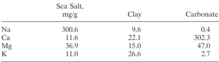
method to exclude non–sea salt contributions to measured Na concentration. Steiger [1991] found the chemical balance method to be more reliable than other approaches used to retrieve the contributions from different aerosol sources from elemental concentrations in a given sample. The method uses a priori information about the elemental composition (i.e., profiles) of different sources and then tries to match the mea-sured composition by a linear combination of the different sources. A least squares minimization procedure was used to match the measured element concentrations of Na, Ca, Mg, and K to varying combinations of sea salt, clay, and/or carbon-ate. The profile for sea salt was chosen as an average seawater composition. Mineral components from clay and carbonate follow the profiles published by Mason and Moore [1982]. Ta-ble 3 lists the profiles chosen for the other components.
With this method the fraction of non–sea salt (NSS) Na averaged over all selected NADP stations for the year 1987 is 8.2% from total Na. The yearly averaged fraction never ex-ceeds 20% at any given site. Hence the correction for non–sea salt should not be a critical source of error for our comparison. The winter use of salt to avoid icing on roads could contribute to observed sea salt concentrations over the continents, but we expect this source to be of minor importance during rainfalls. Deposition fluxes are also measured as part of the European Monitoring and Evaluation Programme (EMEP) over western Europe. The proximity of these stations to the coast renders any attempt of comparison with our model results a much more difficult task.
4.2. Large Sea Salt Particles (Spume Drop Mode)
Large particles (ⱖ4m) are the most difficult to measure. The vertical resolution used in global chemical models limits in the way in which we can account for the large vertical gradients in the number of these particles (the first model layer consists of 70 m). Given this restriction, we will devote only a small part of the model/measurement comparison to these particle sizes. Simulations of these large particles in the marine boundary layer were made by De Leeuw and Davidson [1989]. De Leeuw [1986a] has gathered existing field and laboratory measure-ments of giant particles sampled at heights of⬍2 m asl.
Comparisons to measurements are more relevant above the ⬃2-m-high turbulent buffer zone identified by De Leeuw [1986b]. We selected measurements reported by Smith et al. [1993] made at ⬃14 m asl on a Scotch island, as well as measurements from the North East Atlantic campaign that took place off the Faeroe Islands in October–November 1989 [O’Dowd and Smith, 1993] at⬃18 m asl. Both studies are based on coupling an Active Scattering Aerosol Spectrometer Probe (ASASP) with a Forward Scattering Spectrometer Probe (FSSP) and an additional optical particle counter to measure the sea salt size distributions. The probes were aligned in the
wind and then do not suffer from inlet problems as discussed for the filter samplers above.
De Leeuw [1987] found no consistent decrease in particle
concentrations or shift in size distribution from the sea surface up to⬃15 m for wind speeds ⬎7 m s⫺1. Thus, aside from the
lowest 2 m, the concentration measured at 15 m asl is repre-sentative for the marine boundary layer extending from 2 to 15 m for sustained wind speeds. For lower wind speeds, when sea salt production and turbulent exchange are dampened, large particles disappear from the measurements at 11 m asl [De Leeuw, 1986b].
We are not aware of measurements of the sea salt size distribution at heights above 15 m. Profile measurements of aerosol mass performed near the Hawaiian coast by Blanchard
et al. [1984] and Daniels [1989] show a weak to strong negative
gradient from 10 to 70 m asl. The same gradient is exhibited in measurements at elevations between 10 and 30 m above the open ocean [Exton et al., 1985].
5. Results From Simulations With
the Three Source Functions
Each of the three sea salt source formulations was ran glo-bally in the transport model driven by meteorological fields for 1987. Table 1 presents yearly and global averaged values of sea salt mass, surface area, and number for three size ranges and for each of the model integration.
In the size range 0.5–4m for rdry, sea salt mass differs by
a factor of 2 between the three formulations, whereas the surface and number concentrations vary by a factor of 3 and 1 order of magnitude, respectively. The largest surface area and number concentration are predicted by the Monahan formu-lation since far more of the smaller particles within this size range are produced (see Figures 1 and 2a). The ratio mass/ surface area indicates the average size distribution within a size range. The smaller ratio of mass/aerosol surface area for Monahan in the range 0.5–4m reflects relatively more small particles produced in that formulation than with the ones from SmithHar and Andreas.
Over the whole size spectrum, Andreas yields a total sea salt mass 3 times greater than Monahan and 5 times greater than SmithHar. The main contribution to this mass comes from large particles in 4 to⬃64m range. Above ⬃64 m, Smith-Har predicts the largest flux for particles that are very short lived in the atmosphere (see Figure 1).
6. Discussion of Comparison Model Results and
Observations
In this section we compare the model outputs to all the measurements described in section 4. This comparison ad-dresses the ability of each formulation to reproduce the ob-served sea salt distributions.
6.1. Simulation of Sea Salt Seasonal Cycle
Sites where sea salt measurements had been conducted for at least a full year were selected. For coastal sites the aerosol sampler had to reach at least 20 m above sea level to avoid possible local sea salt production from the surf zone [Savoie
and Prospero, 1977]. Simulated sea salt distributions were
trun-cated above a rdry of 2.9m to reproduce the PM10 inlet of
most of the aerosol samplers in an environment with ⬃80%
Table 3. Element Source Profiles for Cations Used in the Chemical Element Balance Method to Retrieve Sea Salt Na⫹in Wet Deposition Measurements
Sea Salt, mg/g Clay Carbonate Na 300.6 9.6 0.4 Ca 11.6 22.1 302.3 Mg 36.9 15.0 47.0 K 11.0 26.6 2.7
relative humidity. We chose to use the model bins up to a dry radius of 2m for this comparison.
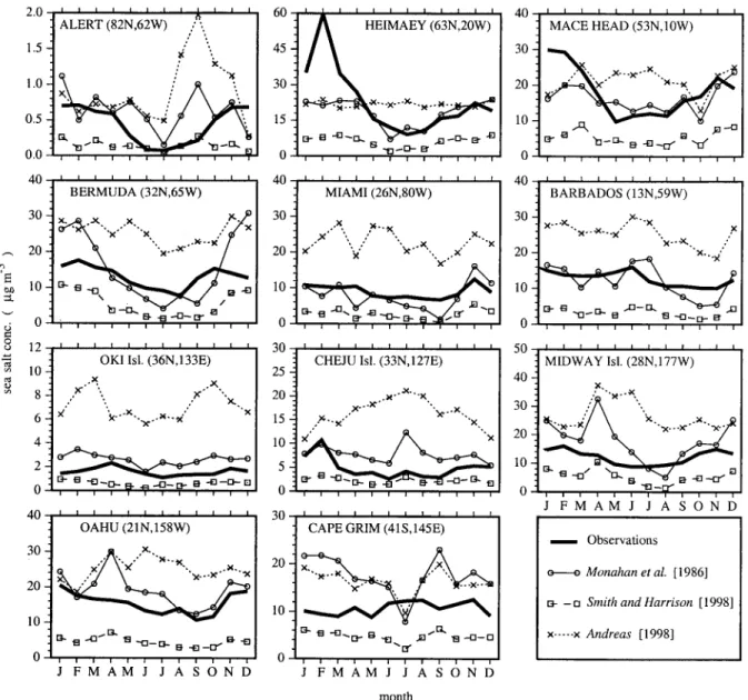
Figure 4 presents the comparison between the observed monthly averaged sea salt concentrations and those simulated with the three formulations at 11 stations. Note the different scales of the y axis. The source formulation Monahan provides the most satisfactory agreement with the observed averaged concentrations. The SmithHar formulation significantly under-estimates concentrations. The formulation from Andreas leads to an overestimate of the average concentrations, which we attribute to a very efficient sea salt production at low wind speeds.
The simulated year was presented for 1987 meteorological fields, whereas measurements could have taken place on a different year or represent an average of several years. This could cause some of the discrepancies seen here.
The most significant discrepancy with Monahan is found at three stations in the Pacific Ocean (Oki, Cheju, and Cape Grim) where the observed sea salt concentration levels are low.
We have not been able to come up with a satisfactory expla-nation for this discrepancy.
Although the Andreas formulation had been adjusted to match the flux produced by Monahan for particles with dry radii below 4 m, Figures 2a and 2b show that production differs substantially according to wind speeds. Monahan’s for-mulation better captures the sharp seasonal features that are observed. This is the case of the pronounced winter maximum observed over the North Atlantic stations or the summer min-imum at North Pacific sites. The maxmin-imum concentration ob-served at Heimaey in February consists of the average of three consecutive years with an extreme value reported for February 13, 1992, of 962g m⫺3sea salt [Gong et al., 1997b].
6.2. Evaluation With Wet Deposition Flux Measurements
Deposition flux measurements are routinely recorded in the framework of NADP network using standard sampling proto-cols. Measurements were made for the year 1987 of the sim-ulation over a large number of North American stations.
Figure 4. Comparisons of monthly averaged sea salt concentrations in surface air (g m⫺3) observed and
simulated with the three formulations at different stations. The model results correspond to particles with
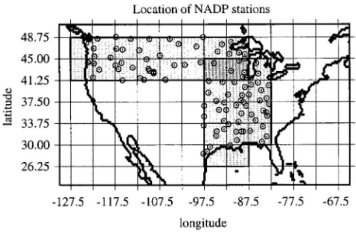
Annual wet deposition fluxes of sea salt measured over the continental United States have been used for this comparison (see section 4.1.2). Selected sites were separated into two groups (Figure 5): a west-east transect with stations located between 41.25⬚N and 48.75⬚N to represent zonal transport of sea salt from the North Pacific and a south-north transect between 82.5⬚W and 97.5⬚W to capture transport of marine air brought about by the cyclones passing over the Gulf of Mexico. Anticyclonic activity over east America is not expected to con-tribute much to sea salt wet fluxes in the inner American regions. Sea salt fluxes should thus reflect the size-dependent removal of sea salt along these two transects.
In Figure 6 we present the comparison between observed and simulated sea salt wet deposition fluxes over the two transects. In this comparison, model deposition fluxes were averaged over the two (respectively three) grid boxes located at the same longitude (respectively latitude). Figure 6 shows a steep decrease of sea salt deposition with the progress of the air mass inland.
The source formulation from SmithHar is in good agree-ment with the observations up to 32⬚N and 115⬚W but a too rapid decrease farther distance from the coast. This result suggests a predominant production of large particles that sed-iment shortly thereafter.
The Andreas’s formulation leads to a similar behavior as SmithHar but with simulated deposition fluxes that are stron-ger. The higher flux from Andreas’s formulation matches the observed deposition far inland, yet it overestimates fluxes in and near the coasts.
The formulation from Monahan brings the gradient into good agreement (⫾35%) with the observations. A larger num-ber of small particles produced can be brought to farther dis-tances than with the others sea salt generation functions.
6.3. Representation of the Larger Particles
Quinn and Coffman [1999] reported measurements over
other regions. We recomputed the simulated number concen-trations for a relative humidity of 70% as reported by Quinn and Coffman. Simulated mass size distributions were averaged
over the corresponding cruise locations for the appropriate months. Figure 7 presents the comparison of measurements taken during these cruises with number concentrations simu-lated with the Monahan formulation. There is a variation of an order of magnitude in mass concentration in the film drop range of the observed size distributions among the different campaigns. The Monahan formulation reproduces well the observed sea salt concentrations up to r70of⬃1m. A
com-parison over the eight size bins of the sea salt distribution agree within ⬃50% to the measured concentration for these small particles.
The simulation for larger particles points out to a significant discrepancy between the model and the measurements for the two upper aerosol impactor stages. Either the Monahan for-mulation overestimates the size range above r70 ⫽ 1 m,
either the collection efficiency of the seven-stage Berner low-pressure impactor is inefficient for these large particles. Howell
et al. [1998] used three different cascade impactors to measure
concurrently the Na⫹size distributions over the open ocean off
the coast of Washington state during the Pacific Sulfur/Stratus Investigation (PSI-91) campaign. This intercomparison showed
Figure 5. Location of the NADP sites (circles) used in this study, where cations in wet deposition have been measured. References to the original measurements are provided in sec-tion 2. The grid corresponds to the model horizontal resolu-tion. The shaded squares correspond to the model grid boxes used for the comparison with NADP measurements, except the lighter shading for which only the coastal measurements are significant.
Figure 6. Comparison between annual sea salt observed and simulated wet deposition fluxes (mg m⫺2d⫺1) with the three
formulations according to the distance in degree from the coast, where the predominant flow of air comes over the con-tinental United States. The simulated values on each grid box have been averaged over the two (respectively three) grid boxes located at the same longitude (respectively latitude), according to the air mass transport as explained in the text. We have drawn a regression line for the observations to show the decreasing trend of sea salt wet deposition with coastal dis-tance.
that the Berner impactor could underestimate sea salt mass by up to a factor of 4 compared to a Sierra impactor. This is close to the disagreement shown in Figure 7. To illustrate it, we show a relatively good agreement between simulated concentrations and measurements made with the Sierra impactor in Figure 8. Here we also discuss results obtained by complementing the distribution simulated by the Monahan formulation for parti-cles with dry radius below 4 m with the SmithHar and An-dreas formulation for greater radii (see section 3.2).
The four data sets mentioned in section 3.3 are used to evaluate the particles of several microns in radius. We ex-tracted simulated instantaneous daily values at noon of sea salt concentrations, retaining those where the wind speed re-mained during the preceding 6 hours time step within one of
the four wind speed classes (5–6 m s⫺1; 8–10 m s⫺1; 15 m s⫺1;
16–17 m s⫺1). Modeled size distributions at a given location
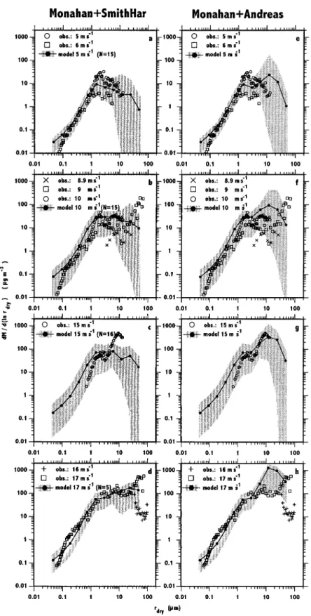
were averaged by wind speed class for the 4 months of obser-vations. All size distributions are presented by mass in Figure 9 and expressed as dry radius to remove the RH dependency from the measurements. Model minimum, maximum, and av-erage concentrations are indicated in Figure 9. The formula-tion Monahan⫹Andreas overestimates the mass of particles ⲏ5m for all wind speeds. A better agreement with observa-tions at all wind speeds is provided by the formulation Monahan⫹SmithHar.
The measurements by O’Dowd et al. [1997b] show a distinct maximum in aerosol mass around 60m which is reproduced in neither simulation (see Figures 9b, 9d, 9f, and 9h). This very
Figure 7. Comparison between the sea salt mass size distributions measured at 70% RH during several open sea campaigns [Quinn and Coffman, 1999] and the monthly averaged size distributions simulated with the Monahan formulation at the same locations and during the same months but for 1987. The x axis represents the particle radius for a RH of 70%.
large mode contributes significantly to the total sea salt mass. Such a mode for the large particles is not seen in the measure-ments of Taylor and Wu [1992] at wind speeds⬎15 m s⫺1(see
Figures 8d and 8h).
7. Sea Salt Surface Area Versus
Total Aerosol Surface Area
One reason for performing the size-resolved sea salt simu-lations is the relevance of the aerosol surface area in hetero-geneous chemistry and for the computation of aerosol radia-tive effects. The relevance of the sea salt aerosol surface area can be illustrated by comparing it to the Earth’s surface area and to the aerosol surface area of the other major aerosol components (sulfate, mineral dust, black carbon, and particu-late organic matter). We will discuss the case where the aerosol is treated as an external mixture.
The sea salt aerosol surface area is computed from the median diameter of each size class and the average density as given in Table 4, which also tabulates the model parameters used for the other aerosol components. Figure 10 shows the global sea salt aerosol surface area as column burden with the Monahan source formulation. Sea salt aerosol surface in ma-rine regions represents 1–10% of the area of the underlying Earth’s surface.
For the comparison with the other aerosol components we combine recent simulations for dust, for black carbon (BC) and particulate organic matter (POM) and sulfate which were performed with the same transport model (TM3) and meteo-rological input fields. The mineral dust simulations were de-scribed by Schulz et al. [1998] and Guelle et al. [1998a] using a dust source described by Claquin [1999] on the basis of the mineralogy of desert areas [Claquin et al., 1999]. The dust source is constrained from detailed investigations of the spatial variability of the threshold velocity in the Saharan region
[Mar-ticorena and Bergametti, 1995], and the occurrence of absorbing
aerosols over desert areas [Herman et al., 1997]. The TM3 simulation for BC and POM was done by C. Liousse (personal communication, 2000) using Liousse et al.’s [1996] source for-mulation. Since both the dust and the BC⫹POM simulation assume a lognormal size distribution, with constant spread but varying median diameter, computation of the aerosol sur-face area is based on the simulated fields of mass and number concentration. The sulfate fields were produced using a de-tailed tropospheric chemistry scheme representing the main species involved in the sulfur cycle and emission inventories for natural and anthropogenic sulfur components [Jeuken, 2000;
Jeuken et al., 2001].
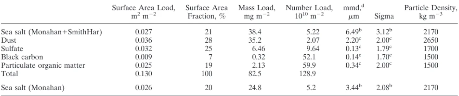
Aerosol loads of the different aerosol components are sum-marized in Table 4. Aerosol surface area, mass, or number are dominated by different aerosol components since each com-ponent has a size distribution with different characteristics. The aerosol surface area is dominated by dust and sulfate followed by the contribution of sea salt and the combined organic aerosol fraction (BC⫹POM). The aerosol mass of mineral dust and sea salt are comparable, exceeding by several folds any other component. In contrast, number concentra-tions are dominated by BC⫹POM and sulfate with a substan-tial contribution from sea salt. The aerosol size distribution of sea salt is much broader than of dust (see Figure 11).
The partitioning of the aerosol surface area among the four aerosol components suggests that one needs to consider every single one to estimate the global aerosol impact on heteroge-neous chemistry and radiative effects. The importance of the sea salt is remarkable in remote marine areas. Sea salt repre-sents 34% of the total aerosol surface area on a yearly average. Plate 1 illustrates the spatial distribution of the sea salt surface area when normalized to the total aerosol surface area. Sea salt is not pervasive relative to other aerosol species over conti-nents and downwind from important continental outflows, east of North America and East Asia, west of Sahara and Central Africa. It becomes much more prominent over southern oceans, where it constitutes the dominant aerosol component.
8. Conclusions
We have evaluated three different sea salt generation func-tions (Monahan, Andreas, and SmithHar) in order to derive the more realistic sea salt distribution for global atmospheric models. Our study was not restricted to a specific size range but rather addressed the whole sea salt size spectrum. This was motivated by the dependence of the radiative effects and the chemistry of sea salt upon the aerosol size.
To evaluate the different source functions, we selected com-plementary observations, so that the model/measurements could be compared for the whole size spectrum. Consideration of humidity effects on particle size and aerosol sampler inlet characteristics is required for a proper comparison between measurements and model results. For instance, we estimated that the aerosol inlets used to measure the seasonal cycle have a cutoff that corresponds to an rdryof 2m. Had we not taken
the cutoff into account, the mean discrepancy between simu-lated and annual observed concentrations would be 77% with Monahan’s formulation,⫹224% with SmithHar, and ⫹1237% with Andreas as compared to 34%, ⫺62%, and ⫹144%, re-spectively.
We showed that the evaluation of the sources requires com-paring results against different observational data sets. For
Figure 8. Comparison between the sea salt mass size distri-bution measured during the PSI-91 campaign with two differ-ent cascade impactors and the one simulated with the Mona-han formulation at the same location and the same month but for 1987.
Figure 9. Simulated sea salt mass size distributions off the west coast of Ireland. The solid lines correspond to the average distribution from 4 months for the wind speed indicated. Minimum and maximum values of simulated distributions during these months form an error envelop, which is shaded. (left) The Monahan⫹SmithHar simulations and (right) the Monahan⫹Andreas formulations. Observations are from De
Leeuw [1987] (crosses), from Taylor and Wu [1992] (pluses), from Smith et al. [1993] (circles), and from O’Dowd et al. [1997b] (squares).
example, in the case of the source formulation from Andreas, the observed sea-salt wet deposition fluxes in the inner conti-nental North America is rather well captured whereas wet deposition and monthly surface level concentrations at the coastal stations are shown to be overestimated.
Sea salt particles with dry radius below 4m are well rep-resented by the Monahan source formulation. We were able to reproduce observations of surface level concentrations, conti-nental wet deposition fluxes, and for size distributions below
rdry⬃ 1–2m.
However, to represent giant sea salt particles, a combination of Monahan and SmithHar is required to have a complete sea salt generation function. The latter formulation shows agreement with the few measured size distributions in the very coarse size
range (rdryup to 80m). However, as previously pointed out by O’Dowd et al. [1997b], measurements of the sea salt size
distribu-tion that extend to large particles are very sparse.
The sea salt simulations are relevant for realistic modeling of heterogeneous chemistry and radiative effects. Sea salt aerosol provides, on an annual average, 21% of the aerosol surface area. Nearly equal partitioning of the aerosol surface area among the four components confirms the necessity to consider all of them to determine the global impact of aerosol on climate and tropo-spheric chemistry.
Future work will use the reanalyzed meteorological fields from ECMWF over either the 15 or 40 year period. This will allow us to better capture the wind-generated fluxes and trans-port fields that were present at the time of the observations. A
Figure 10. Annual average of sea salt aerosol surface area per Earth surface area using the source formu-lation Monahan.
Table 4. Annual Global Average of Daily Values From TM3 Simulations of This Studya
Surface Area Load,
m2m⫺2 Surface AreaFraction, % Mass Load,mg m⫺2 Number Load,1010m⫺2 mmd, d
m Sigma Particle Density,kg m⫺3
Sea salt (Monahan⫹SmithHar) 0.027 21 38.4 5.22 6.49b 3.12b 2170
Dust 0.036 28 35.2 2.07 2.20c 2.00c 2650
Sulfate 0.032 25 6.46 9.64 0.13c 1.79c 1700
Black carbon 0.009 7 0.32 52.1 0.14c 1.70c 1500
Particulate organic matter 0.025 19 2.13 59.9 0.34c 2.00c 1500
Total 0.130 100 82.5 128.9
Sea salt (Monahan) 0.026 20 24.8 5.2 3.44b 2.08b 2170
aGlobal areal average of column integrated data (N⫽ 72*48). bSize distribution parameters are computed from binned data. cSize distribution parameters correspond to a lognormal distribution. dmmd, mass median diameter.
Plate 1. Comparison of sea salt aerosol surface area to total aerosol surface area including mineral dust, black carbon, particulate organic matter, and sulfate.
quantitative study will focus on the interannual variability of the sea salt distribution based upon the source function (Monahan⫹SmithHar).
Appendix A
The mathematical formulations of the three source functions used in this study are presented. The fluxes F are expressed in particles [m⫺1m⫺2s⫺1], r corresponds to the particle radius in
[m], and U10to the wind speed at 10-m height [m s⫺1].
The sea salt generation function given by Monahan et al. [1986] for particles with radius ⱗ10 m and referenced as SmithHar in the paper is formulated as follows:
dF/dr⫽ 1.373U103.41r⫺3共1 ⫹ 0.057r1.05兲101.19exp共⫺B2兲, (A1)
where B ⫽ (0.38 ⫺ log10r)/0.65
The sea salt generation function given by Smith and Harrison [1998] and referenced as SmithHar in the paper is formulated as follows: dF dr ⫽
冘
i⫽1 2 Aiexp冋
⫺filn冉
r r0i冊
2册
, (A2)where r01⫽ 3m and r02⫽ 30m, f1⫽ 1.5 and f2⫽ 1, and
coefficients A1and A2 are approximated by A1 ⫽ 0.2 U103.5
and A2 ⫽ 6.8 10⫺3 U103 .
The sea salt generation function proposed by Andreas [1998] (referenced as Andreas in the paper) uses the Smith et al. [1993] source for particles with r ⱕ 10 m, corrected for an effective wind speed U14measured at 14 m asl. This generation
function uses the same formula as in (A2) multiplied by a factor of 3.5 but with r01⫽ 2.1m and r02⫽ 9.2m, f1⫽ 3.1
and f2⫽ 3.3, and coefficients A1and A2defined as
A1⫽ 10共0.0676 U14⫹2.43兲 (A3)
A2⫽ 10共0.959 U14
0.5⫺1.476兲
(A4) with the wind speed U14expressed as a function of the 10-m
wind speed through
U14⫽ U10
冋
1⫹ CDN100.50.4 ln
冉
1410
冊册
, (A5) where the neutral-stability drag coefficient is given byCDN10⫽
再
1.20⫻ 10⫺3 4ⱕ U
10ⱕ 11 m s⫺1
共0.49 ⫹ 0.064 U10兲10⫺3 U10ⱖ 11 m s⫺1
(A6) For particles larger than 10m in radius the Andreas [1998] source is based on Andreas [1992] work and is formulated as
dF dr ⫽ C1U10r⫺1 10ⱕ r ⱕ 37.5m (A7a) dF dr ⫽
再
C1U10r⫺1 10ⱕ r ⱕ 37.5m C2U10r⫺2.8 37.5ⱕ r ⱕ 100 m. (A7b)Acknowledgments. We would like to thank Martin Heimann for providing access to and expertise of the TM3 code. Cathy Liousse and Tanguy Claquin kindly made available their simulation results for carbonaceous and mineral dust aerosols. Computing resources were provided by the Commissariat a` l’Energie Atomique. For advice and supply of observational data we are most grateful to Joe Prospero and Gerrit de Leeuw. The National Atmospheric Deposition Program (NADP/NTN) kindly made that program’s data available on their web site (http://nadp.sws.uiuc.edu/default.html). Funding of postdoctoral work was granted through the EU-ENVIRONMENT & CLIMATE project SINDICATE (contract ENV4-CT95-0099) and the German Aerosol Research Programme (BMBF Foerderkennzeichen 07 AF 312 B/7). This is LSCE contribution 0660.
References
Andreas, E. L., Sea spray and the turbulent air-sea heat fluxes, J.
Geophys. Res., 97, 11,429–11,441, 1992.
Andreas, E. L., A new sea spray generation function for wind speeds up to 32 m s⫺1, J. Phys. Oceanogr., 28, 2175–2184, 1998.
Andreas, E. L., J. B. Edson, E. C. Monahan, M. P. Rouault, and S. D. Smith, The spray contribution to net evaporation from the sea: A review of recent progress, Boundary Layer Meteorol., 72, 3–52, 1995. Behnke, W., C. George, V. Sheer, and C. Zetzsch, Production and decay of ClNO2 from the reaction of gaseous N2O5 with NaCl
solution: Bulk and aerosol experiments, J. Geophys. Res., 102, 3795– 3804, 1997.
Blanchard, D. C., A. H. Woodcock, and R. J. Cipriano, The vertical distribution of sea salt in the marine atmosphere near Hawaii,
Tel-lus, Ser. B, 36, 118–125, 1984.
Carmichael, G. R., Y. Zhang, L. Chen, M. Hong, and H. Ueda, Sea-sonal variation of aerosol composition at Cheju Island, Korea,
At-mos. Environ., 30, 2407–2416, 1996.
Chameides, W. L., and A. W. Stelson, Aqueous-phase chemical pro-cesses in deliquescent sea-salt aerosols: A mechanism that couples the atmospheric cycles of S and sea salt, J. Geophys. Res., 97, 20,565– 20,580, 1992.
Claquin, T., Mode´lisation de la mine´ralogie et du forc¸age radiatif des poussie`res de´sertiques. Ph.D. thesis, Univ. de Paris VI/FB Chem. der Univ. Hamburg, Paris, 1999.
Claquin, T., M. Schulz, and Y. Balkanski, Modeling the mineralogy of atmospheric dust sources, J. Geophys. Res., 104, 22,243–22,256, 1999. Daniels, A., Measurements of atmospheric sea salt concentrations in
Hawaii using a Tala kit, Tellus, Ser. B, 41, 196–206, 1989. De Leeuw, G., Size distributions of giant aerosol particles close above
sea level, J. Aerosol Sci., 17, 293–296, 1986a.
De Leeuw, G., Vertical profiles of giant particles close above the sea surface, Tellus, Ser. B, 38, 51–61, 1986b.
De Leeuw, G., Near-surface particle size distributions profiles over the North Sea, J. Geophys. Res., 92, 14,631–14,635, 1987.
De Leeuw, G., and K. L. Davidson, Aerosol modeling in the marine atmospheric boundary layer, in Man and His Ecosystem. Proceedings
of the 8th World Clean Air Congress, The Hague, The Netherlands,
11–15 Sept. 1989, vol. 3, edited by L. J. Brasser and W. C. Mulder, pp. 617–622, Elsevier Sci., New York, 1989.
Denning, A. S., et al., Three-dimensional transport and concentration of SF6: A model intercomparison study (TransCom 2), Tellus, Ser. B,
51, 266–297, 1999.
Dentener, F., J. Feichter, and A. Jeuken, Simulation of the transport
Figure 11. Global and annual average mass load of sea salt and dust against particle size.
of Rn using on-line and off-line global models at different hori-zontal resolutions: A detailed comparison with measurements,
Tel-lus, Ser. B, 51, 573–602, 1999.
Erickson, D. J., J. T. Merrill, and R. A. Duce, Seasonal estimates of global atmospheric sea-salt distributions, J. Geophys. Res., 91, 1067– 1072, 1986.
Erickson, D. J., C. Seuzaret, W. C. Keene, and S. L. Gong, A general circulation model based calculation of HCl and ClNO2production
from sea salt dechlorination: Reactive chlorine emissions inventory,
J. Geophys. Res., 104, 8347–8372, 1999.
Exton, H. J., J. Latham, P. M. Park, S. J. Perry, M. H. Smith, and R. R. Allan, The production and dispersal of marine aerosol, Q. J. R.
Meteorol. Soc., 111, 817–837, 1985.
Finlayson-Pitts, B. J., Reaction of N2O5with NaCl and atmospheric
implications of NOCl formation, Nature, 306, 676–677, 1983. Finlayson-Pitts, B. J., M. J. Ezell, and J. N. Pitts Jr., Formation of
chemically active chlorine compounds by reactions of atmospheric NaCl particles with gaseous N2O5and ClNO2, Nature, 337, 241–244,
1989.
Fitzgerald, J. W., Marine aerosols: A review, Atmos. Environ., Part A,
25, 533–545, 1991.
Francois, F., W. Maenhaut, J.-L. Colin, R. Losno, M. Schulz, T. Stahl-schmidt, L. Spokes, and T. Jickells, Intercomparison of elemental concentrations in total and size-fractionated aerosol samples col-lected during the Mace Head experiment, April 1991. Atmos.
Envi-ron., 29, 837–849, 1995.
Genthon, C., Simulations of desert dust and sea-salt aerosols in Ant-arctica with a general circulation model of the atmosphere, Tellus,
Ser. B, 44, 371–389, 1992.
Gerber, H., Relative humidity parameterization of the lognormal size distribution of ambient aerosols, in Atmospheric Aerosols and
Nu-cleation, Lect. Notes Phys., vol. 309, edited by P. E. Wagner and G.
Vali, pp. 237–238, Springer-Verlag, New York, 1988.
Gong, S. L., L. A. Barrie, and J.-P. Blanchet, Modeling sea-salt aero-sols in the atmosphere, 1, Model development, J. Geophys. Res., 102, 3805–3818, 1997a.
Gong, S. L., L. A. Barrie, J. M. Prospero, D. L. Savoie, G. P. Ayers, J.-P. Blanchet, and S. Lubos, Modeling sea-salt aerosols in the at-mosphere, 2, Atmospheric concentrations and fluxes, J. Geophys.
Res., 102, 3819–3830, 1997b.
Guelle, W., Y. J. Balkanski, M. Schulz, F. Dulac, and P. Monfray, Wet deposition in a global size-dependent aerosol transport model, 1, Comparison of a 1 year210Pb simulation with ground measurements,
J. Geophys. Res., 103, 11,429–11,445, 1998a.
Guelle, W., Y. J. Balkanski, J. Dibb, M. Schulz, and F. Dulac, Wet deposition in a global size-dependent aerosol transport model, 2, Influence of the scavenging scheme on210Pb vertical profiles,
sur-face concentrations and deposition, J. Geophys. Res., 103, 28,875– 29,891, 1998b.
Guelle, W., Y. J. Balkanski, M. Schulz, B. Marticorena, G. Bergametti, C. Moulin, R. Arimoto, and K. D. Perry, Modeling the atmospheric distribution of mineral aerosol: Comparison with ground measure-ments and satellite observations for yearly and synoptic timescales over the North Atlantic, J. Geophys. Res., 105, 1997–2012, 2000. Gurciullo, C., B. Lerner, H. Sievering, and S. N. Pandis,
Heteroge-neous sulfate production in the remote marine boundary environ-ment: Cloud processing and sea-salt particle contributions, J.
Geo-phys. Res., 104, 21,719–21,731, 1999.
Haywood, J. M., V. Ramaswamy, and B. J. Soden, Tropospheric aero-sol climate forcing in clear-sky satellite observations over the oceans,
Science, 283, 1299–1303, 1999.
Heimann, M., The global atmospheric model TM2, Tech. Rep. 10, Dtsch. Klimarechenzent., Modellbetreuungsgruppe, Hamburg, Ger-many, 1995.
Herman, J. R., P. K. Bathia, O. Torres, C. Hsu, C. Seftor, and E. Celarier, Global distribution of UV-absorbing aerosols from Nim-bus 7/TOMS data, J. Geophys. Res., 102, 16,911–16,922, 1997. Houweling, S., F. Dentener, and J. Lelieveld, The impact of
nonmeth-ane hydrocarbon compounds on tropospheric photochemistry, J.
Geophys. Res., 103, 10,673–10,696, 1998.
Howell, S., A. A. P. Pszenny, P. Quinn, and B. Huebert, A field intercomparison of three cascade impactors, Aerosol Sci. Technol.,
29, 475–492, 1998.
Jeuken, A., Evaluation of chemistry and climate models using mea-surements and data assimilation. Ph.D. thesis, KNMI/Tech. Univ. Eindhoven, Eindhoven, Netherlands, 2000.
Jeuken, A. B., M. P. Veefkind, F. J. Dentener, S. Metzger, and C. Robles Gonzalez, Simulation of the aerosol optical depth over Eu-rope for August 1997 and a comparison with observations, J.
Geo-phys. Res., in press, 2001.
Latham, J., and M. H. Smith, Effect on global warming of wind-dependent aerosol generation at the ocean surface, Nature, 347, 372–373, 1990.
Lelieveld, J., and F. Dentener, What controls tropospheric ozone?, J.
Geophys. Res., 105, 3531–3551, 2000.
Liousse, C., J. E. Penner, C. Chuang, J. J. Walton, and H. Eddleman, A global three-dimensional model study of carbonaceous aerosols, J.
Geophys. Res., 101, 19,411–19,432, 1996.
Lovett, R. F., Quantitative measurement of airborne sea-salt in the North Atlantic, Tellus, Ser. B, 30, 358–364, 1978.
Marticorena, B., and G. Bergametti, Modelling the atmospheric dust cycle, 1, Design of a soil-derived dust emission scheme, J. Geophys.
Res., 100, 16,415–16,430, 1995.
Mason, B., and C. Moore, Principles of Geochemistry, John Wiley, New York, 1982.
Monahan, E. C., D. E. Spiel, and K. L. Davidson, A model of marine aerosol generation via whitecaps and wave disruption, in Oceanic
Whitecaps and Their Role in Air-Sea Exchange, edited by E. C.
Mona-han and G. Mac Niocaill, pp. 167–174, D. Reidel, Norwell, Mass., 1986.
Mukai, H., and M. Suzuki, Using air trajectories to analyze the sea-sonal variation of aerosols transported to the Oki Islands, Atmos.
Environ., 30, 3917–3934, 1996.
Murphy, D. M., J. R. Anderson, P. K. Quinn, L. M. McInnes, F. J. Brechtel, S. M. Kreidenweis, A. M. Middlebrook, M. Po´sfai, D. S. Thomson, and P. R. Buseck, Influence of sea-salt on aerosol radia-tive properties in the Southern Ocean marine boundary layer,
Na-ture, 392, 62–65, 1998.
O’Dowd, C. D., and M. H. Smith, Physicochemical properties of aero-sols over the northeast Atlantic: Evidence for wind-speed-related submicron sea-salt aerosol production, J. Geophys. Res., 98, 1137– 1149, 1993.
O’Dowd, C. D., J. A. Lowe, M. H. Smith, B. Davison, C. N. Hewitt, and R. M. Harrison, Biogenic sulphur emissions and inferred non–sea-sulphate cloud condensation nuclei in and around Antarctica, J.
Geophys. Res., 102, 12,839–12,854, 1997a.
O’Dowd, C. D., M. H. Smith, I. E. Consterdine, and J. A. Lowe, Marine aerosol, sea-salt, and the marine sulphur cycle: A short review, Atmos. Environ., 31, 73–80, 1997b.
O’Dowd, J. A. Lowe, M. H. Smith, and A. D. Kaye, The relative importance of non-sea-salt sulphate and sea-salt aerosol to the ma-rine cloud condensation nuclei population: An improved multi-component aerosol-cloud droplet parameterization, Q. J. R.
Meteo-rol. Soc., 556, 1295–1314, 1999a.
O’Dowd, J. A. Lowe, and M. H. Smith, Coupling sea-salt and sulphate interactions and its impact on cloud droplet concentration predic-tions, Geophys. Res. Lett., 26, 1311–1314, 1999b.
Prospero, J. M., Long-term measurements of the transport of African mineral dust to the southeastern United States: Implications for regional air quality, J. Geophys. Res., 104, 15,917–15,927, 1999. Quinn, P. K., and D. J. Coffman, Comment on “Contribution of
dif-ferent aerosol species to the global aerosol extinction optical thick-ness: Estimates from model results” by I. Tegen et al., J. Geophys.
Res., 104, 4241–4248, 1999.
Quinn, P. K., D. S. Covert, T. S. Bates, V. N. Kapustin, D. C. Ramsey-Bell, and L. M. McInnes, Dimethylsulfide/cloud condensation nu-clei/climate system: Relevant size-resolved measurements of the chemical and physical properties of atmospheric aerosol particles, J.
Geophys. Res., 98, 10,411–10,427, 1993.
Savoie, D. L., and J. M. Prospero, Aerosol concentration statistics for the northern tropical Atlantic, J. Geophys. Res., 82, 5954–5964, 1977. Schulz, M., Y. Balkanski, W. Guelle, and F. Dulac, Treatment of aerosol size distribution in a global transport model: Validation with satellite-derived observations for a Saharan dust episode, J. Geophys.
Res., 103, 10,579–10,592, 1998.
Sievering, H., J. Boatman, J. Galloway, W. Keene, Y. Kim, M. Luria, and J. Ray, Heterogeneous sulfur conversion in sea-salt aerosol particles: The role of aerosol water content and size distribution,
Atmos. Environ., 25, 1479–1487, 1991.
Sievering, H., J. Boatman, E. Gorman, Y. Kim, L. Anderson, G. Ennis, M. Luria, and S. Pandis, Removal of sulphur from the marine
boundary layer by ozone oxidation in sea-salt aerosols, Nature, 360, 571–573, 1992.
Smith, M. H., and N. M. Harrison, The sea spray generation function,
J. Aerosol Sci., 29, Suppl. 1, S189–S190, 1998.
Smith, M. H. and C. D. O’Dowd, Observations of accumulation model aerosol composition and soot carbon concentrations by means of the high-temperature volatility technique, J. Geophys. Res., 101, 19,583– 19,591, 1996.
Smith, M. H., P. M. Park, and I. E. Consterdine, Marine aerosol concentrations and estimated fluxes over the sea, Q. J. R. Meteorol.
Soc., 119, 809–824, 1993.
Steiger, M., Die antropogenen und natu¨rlichen Quellen urbaner und mariner Aerosole charakterisiert und quantifiziert durch Multiele-mentanalyse und chemische Receptormodelle. Ph.D. thesis, Fach-ber. Chem., Univ. Hamburg, Hamburg, Germany, 1991.
Taylor, N. J., and J. Wu, Simultaneous measurements of spray and sea salt, J. Geophys. Res., 97, 7355–7360, 1992.
Tegen, I., P. Hollrig, M. Chin, I. Fung, D. J. Jacob, and J. E. Penner, Contribution of different aerosol species to the global aerosol ex-tinction optical thickness: Estimates from model results, J. Geophys.
Res., 102, 23,895–23,915, 1997.
van den Berg, A., F. Dentener, and J. Lelieveld, Modeling the chem-istry of the marine boundary layer; sulphate formation and the role of sea salt aerosol particles, J. Geophys. Res., 105, 11,671–11,698, 2000.
Wu, J., J. J. Murray, and R. J. Lai, Production and distributions of sea spray, J. Geophys. Res., 89, 8163–8169, 1984.
Zwally, H. J., J. C. Comiso, C. L. Parkinson, W. J. Campbell, F. D. Carsey, and P. Gloersen, Antarctic sea ice, 1973–1976: Satellite passive microwave observations, NASA Spec. Publ., SP-469, 206 pp., 1983.
Y. Balkanski, W. Guelle, and M. Schulz, Laboratoire des Sciences du Climat et de l’Environnement, L’Ormes des Merisiers, Bat. 709, F-91191 Gif-sur-Yvette Cedex, France. ([email protected])
F. Dentener, European Commission, Joint Research Centre, Bldg 29, Via Enrico Fermi, I-21020 Ispra, Italy. ([email protected])
(Received July 10, 2000; revised May 18, 2001; accepted May 24, 2001.)