Simulation of stratospheric water vapor trends: impact on stratospheric ozone chemistry

(1)

HAL Id: hal-00301462

https://hal.archives-ouvertes.fr/hal-00301462

Submitted on 14 Oct 2004

HAL is a multi-disciplinary open access

archive for the deposit and dissemination of sci-entific research documents, whether they are pub-lished or not. The documents may come from teaching and research institutions in France or abroad, or from public or private research centers.

L’archive ouverte pluridisciplinaire HAL, est destinée au dépôt et à la diffusion de documents scientifiques de niveau recherche, publiés ou non, émanant des établissements d’enseignement et de recherche français ou étrangers, des laboratoires publics ou privés.

Simulation of stratospheric water vapor trends: impact

on stratospheric ozone chemistry

A. Stenke, V. Grewe

To cite this version:

A. Stenke, V. Grewe. Simulation of stratospheric water vapor trends: impact on stratospheric ozone chemistry. Atmospheric Chemistry and Physics Discussions, European Geosciences Union, 2004, 4 (5), pp.6559-6602. �hal-00301462�

(2)

ACPD

4, 6559–6602, 2004 Impact of stratospheric water vapor trends on ozone chemistry

A. Stenke and V. Grewe

Title Page Abstract Introduction Conclusions References Tables Figures J I J I Back Close Full Screen / Esc

Print Version Interactive Discussion

www.atmos-chem-phys.org/acpd/4/6559/ SRef-ID: 1680-7375/acpd/2004-4-6559 © European Geosciences Union 2004

Atmospheric Chemistry and Physics Discussions

Simulation of stratospheric water vapor

trends: impact on stratospheric ozone

chemistry

A. Stenke and V. Grewe

Deutsches Zentrum f ür Luft- und Raumfahrt (DLR), Institut f ür Physik der Atmosph äre, Oberpfaffenhofen, D-82234 Weßling, Germany

Received: 16 August 2004 – Accepted: 5 October 2004 – Published: 14 October 2004 Correspondence to: A. Stenke (andrea.stenke@dlr.de)

(3)

ACPD

Abstract

A transient model simulation from 1960 to 2000 with the coupled climate-chemistry model (CCM) ECHAM4.L39(DLR)/CHEM shows a stratospheric water vapor trend dur-ing the last two decades of +0.7 ppmv and additionally a short-term increase during volcanic eruptions. At the same time this model simulation shows a long-term decrease

5

in total ozone and a short-term tropical ozone decline after a volcanic eruption. In or-der to unor-derstand the resulting effects of the water vapor changes on stratospheric ozone chemistry, different perturbation simulations have been performed with the CCM ECHAM4.L39(DLR)/CHEM with the water vapor perturbations fed only to the chem-istry part. Two different long-term perturbations of stratospheric water vapor, +1 ppmv

10

and+5 ppmv, and a short-term perturbation of +2 ppmv with an e-folding time of two months have been simulated. Since water vapor acts as an in-situ source of odd hydro-gen in the stratosphere, the water vapor perturbations affect the gas-phase chemistry of hydrogen oxides. An additional water vapor amount of+1 ppmv results in a 5–10% OH increase. Coupling processes between HO_x and NO_x/ClO_x also affect the ozone

15

destruction by other catalytic reaction cycles. The HO_x cycle becomes 6.4% more ef-fective, whereas the NO_xcycle is 1.6% less effective. A long-term water vapor increase does not only affect the gas-phase chemistry, but also the heterogeneous ozone chem-istry in polar regions. The additional water vapor intensifies the strong denitrification of the Antarctic winter stratosphere caused by an enhanced formation of polar

strato-20

spheric clouds. Thus it further facilitates the catalytic ozone removal by the ClO_xcycle. The reduction of total column ozone during Antarctic spring peaks at −3%. In contrast, heterogeneous chemistry during Arctic winter is not affected by the water vapor in-crease. The short-term perturbation studies show similar patterns, but because of the short perturbation time, the chemical effect on ozone is almost negligible. Finally, this

25

study shows that 10% of the simulated long-term ozone decline in the transient model simulation can be explained by the water vapor increase, but the simulated tropical ozone decrease after volcanic eruptions is caused dynamically rather than chemically.

(4)

ACPD

1. Introduction

Water vapor in the upper troposphere (UT) and lower stratosphere (LS) plays a key role in atmospheric chemistry. The oxidation of H₂O and CH₄ by excited oxygen O(1D) is the primary source of hydrogen oxides (HOx=OH+HO2) (ReactionR1–R2), which are involved in an important catalytic reaction cycle that controls the production and de-struction of ozone in the lower stratosphere. The importance of the catalytic HO_x-cycles for the photochemistry of stratospheric O₃has already been identified in 1950 byBates and Nicolet. Additionally, OH is important for changing the partitioning of the nitrogen and the halogen family which are crucial for the O₃removal in the stratosphere.

O(1D)+ H2O → 2OH (R1)

O(1D)+ CH4→ OH+ CH3 (R2)

Several studies discussed an increase in stratospheric water vapor (Evans et al., 1998; Michelsen et al., 2000; Nedoluha et al., 1998; Rosenlof, 2002). For exam-ple,Rosenlof et al.(2001) combined ten different data sets between 1954 and 2000, and examined a trend of +1%/yr. Several reasons like enhanced methane

oxida-5

tion, increased aircraft emission in the LS, a warming of the tropical tropopause, vol-canic eruptions and large-scale changes in stratospheric circulation and troposphere-stratosphere-exchange have been discussed, but the observed stratospheric water va-por increase is not yet understood (Evans et al., 1998, and references therein). In contrast, tropical tropopause temperatures have been found to decrease (Zhou et al.,

10

2001).

Oltmans et al. (2000) analyzed 20 years of water vapor measurements with the NOAA Climate Monitoring and Diagnostics Laboratory (CMDL) frostpoint hygrometer over Boulder, CO, and reported a+1%/yr (+0.05 ppmv/yr) trend in the stratosphere. Figure1shows a comparison of this time series with a corresponding water vapor time

15

series from a transient model simulation with ECHAM4.L39(DLR)/CHEM1. The model

1

(5)

ACPD

(2001) stated that the water vapor minimum above the tropical tropopause is qualita-tively reproduced, but stratospheric water vapor mixing ratios are systematically over-estimated by ECHAM4.L39(DLR)/CHEM. Both time series show a positive linear trend. The water vapor trend over Boulder (24–26 km) is +0.044±0.012 ppmv/yr (Oltmans

5

et al.,2000). The simulated water vapor trend is 35% weaker than the observed trend. It amounts to+0.029±0.007 ppmv/yr. The uncertainties are the 95% confidence in-tervals using the t-statistic. At the same time the model results show a decrease in global mean total column ozone of approximately −1.7%/decade (−5.5 DU/decade). Several studies have shown that increasing stratospheric water vapor affects the ozone

10

budget significantly (e.g.Evans et al.,1998;Dvortsov and Solomon,2001). Figure2a shows the trend in ozone in the transient model simulation, which is similar to observed values (WMO, 2002). One objective of this study is to assess the contribution of the simulated water vapor increase to the analyzed ozone decrease.

The model results show two pronounced water vapor peaks, associated with the

15

eruption of the volcanos El Chichon (17.33◦N, 93.20◦W) in 1982 and Mount Pinatubo (15.13◦N, 120.35◦E) in 1991 (Fig. 1). The observations over Boulder also show en-hanced water vapor mixing ratios in 1992 after the Pinatubo eruptions as indicated by the dashed line in Fig.1. The volcanic eruptions lead to a short-term increase of strato-spheric water vapor. In the model simulation the water vapor mixing ratios return to

pre-20

volcanic levels 2 years after the maximum value. Since both volcanos are located in the tropics within the upwelling branch of the Brewer-Dobson circulation, it is expected that the gas-phase chemistry of the tropical lower stratosphere is primarily influenced by a short-term increased water vapor loading. Several effects of the volcanic eruption of Mount Pinatubo on the stratospheric water vapor have been discussed. Beside the

di-25

rect injection of large amounts of water vapor into the stratosphere (Glaze et al.,1997), volcanic eruptions cause an enhanced sulphate aerosol loading which results in an important heating effect on the tropical tropopause (Stenchikov et al.,1998). A warmer simulation with a chemistry-climate model employing realistic forcings, to be submitted in ACP.

(6)

ACPD

stratosphere (Considine et al., 2001). Figure 2b shows the simulated tropical ozone decline after the last three major volcanic eruptions. Beside the ozone trend analysis a second major objective is to investigate whether these short-term ozone changes arise from a short-term water vapor increase.

5

The effect of increasing stratospheric water vapor on ozone chemistry has also been discussed within the scope of supersonic aircraft emission studies.Gauss et al.(2003) analyzed the impact of water vapor emissions from aircraft on the atmosphere with a chemical transport model for the year 2015. They found that supersonic aircraft cause a pronounced water vapor perturbation in the lower stratosphere with values

10

up to +400 ppbv (their Figure 8). Gauss et al. (2003) considered the stratospheric water vapor emissions as a passive tracer without chemical loss and applied a tropo-spheric lifetime of 8.75 days. Morris et al.(2003) applied a trajectory model to assess stratospheric water vapor changes caused by sub- and supersonic aircraft. They sim-ulated maximum water vapor perturbations of 1.5 ppmv in the tropical stratosphere

15

near 20 km. Since the only loss mechanism for water vapor considered in the simula-tions is transport to the troposphere,Morris et al.(2003) stated that the results should be viewed as upper limit. The impact of supersonic H₂O emissions on stratospheric ozone has been studied with various 2D- and 3D-CTMs inIPCC(1999). In contrast to the present study theIPCCmodel studies do not include detailed analyses of chemical

20

processes and their changes caused by the H₂O perturbation.

In this paper we investigate the impact of increased stratospheric water vapor on stratospheric ozone chemistry by model simulations with the coupled climate-chemistry model ECHAM4.L39(DLR)/CHEM. We use a special method to prevent a feedback of the simulated water vapor increase to the model dynamics in order to separate the

25

chemical effect. A short model description is given in the next section. Section3 de-scribes the applied tracer approach. The results of our study are presented in Sec.4.1 and4.2. We differentiate between a short-term and a long-term water vapor increase. A discussion and summary is given in the last section.

(7)

ACPD

2. Model description

The coupled climate-chemistry model ECHAM4.L39(DLR)/CHEM (Hein et al., 2001, hereafter referred to as E39/C) consists of the dynamic part ECHAM4.L39(DLR) (E39) and the chemistry module CHEM. E39 is a spectral general circulation model, based on the climate model ECHAM4 (Roeckner et al.,1996), and has a vertical resolution

5

of 39 levels up to the top layer centered at 10 hPa (Land et al., 1999). A horizontal resolution of T30 (≈6◦ isotropic resolution) is used in this study. The tracer transport, parameterizations of physical processes and the chemistry are calculated on the cor-responding Gaussian transform grid with a grid size of 3.75◦×3.75◦. Water vapor, cloud water and chemical species are advected by a so-called semi-Lagrangian scheme.

10

The chemistry module CHEM (Steil et al., 1998) is based on the family concept. It includes stratospheric homogeneous and heterogeneous ozone chemistry and the most relevant chemical processes for describing the tropospheric background NO_x -CH₄-CO-HO_x-O₃ chemistry with 107 photochemical reactions, 37 chemical species and 4 heterogeneous reactions on polar stratospheric clouds (PSCs) and on sulphate

15

aerosols. CHEM does not yet consider bromine chemistry. Mixing ratios of methane (CH₄), nitrous oxide (N₂O) and carbon monoxide (CO) are prescribed at the surface followingIPCC(2001) for the year 2000. Zonally averaged monthly mean concentra-tions of chlorofluorocarbons (CFCs) and upper boundary condiconcentra-tions for total chlorine and total nitrogen are taken from the 2-D model ofBr ¨uhl and Crutzen(1993). Nitrogen

20

oxide emissions at the surface (natural and anthropogenic sources), from lightning and aircraft are considered. The model set-up followsHein et al.(2001) except for the total amounts of emissions, lightning NO_x, which is parameterized according toGrewe et al. (2001), and a more detailed sulphate aerosol chemistry.

The model E39/C can be run in two different modes: with- and without-feedback. In

25

the without-feedback mode the concentrations of the radiatively active gases H₂O, O₃, N₂O, and CFCs calculated by CHEM do not feed back to the radiative scheme of E39. Prescribed climatological mixing ratios of the radiatively active gases are used as input

(8)

ACPD

(2001).

The hydroxyl radical (OH) plays a crucial role for the present study. Since the model climatology given inHein et al. (2001) does not consider OH, the OH distribution in E39/C will be discussed below. Figure3 shows a vertical cross-section of the zonally

5

and monthly averaged OH distribution in E39/C. Because of the extreme variability of OH in time and space due to the high dependency on the solar zenith angle (Hanisco et al.,2001), it is inappropriate to compare in situ OH measurements (e.g.Wennberg et al., 1995) with model results which include night hours. Spivakovsky et al. (2000) calculated a global climatological distribution of tropospheric OH (referred to OH-S

10

hereafter) using observations of precursors for OH like O₃, H₂O, CO, hydrocarbons and NO_t (defined as NO₂+ NO + 2N2O₅+ NO3+ HNO2+ HNO4,Spivakovsky et al., 2000) as well as observed temperatures and cloud optical depths as input for a photo-chemical box model. OH-S shows the highest zonal mean OH concentrations in the tropics at ca. 600 hPa, peaking at about 25×105 molecules/cm3. Within this altitude

15

range the tropical OH concentrations in E39/C are in good agreement with OH-S. The OH distribution in E39/C has a maximum closer to the surface. This might be associ-ated with the missing effects of non-methane-hydrocarbons (NMHCs) on OH in E39/C. OH is depleted over forested tropical continents by the influence of NMHCs (Lawrence et al.,2001). In both OH distributions the maximum OH concentrations are shifted to

20

the respective summer hemisphere during January and July, following the position of the sun. During April and October both OH distributions are mostly hemispherically symmetric. The mid-latitudes exhibit a strong seasonal cycle that is associated with sunlight and water vapor variations. Both OH distributions show very low OH concen-trations at high latitudes during winter. OH-S shows a more pronounced vertical

gradi-25

ent between 500 and 100 hPa. Hence E39/C overestimates the OH concentrations in this altitude range. Generally, the comparison of both OH distributions shows that for the matter of this study the modeled OH distribution is realistically enough reproduced.

(9)

ACPD

3. Methodology

3.1. Water vapor perturbations

The intention of this study is to investigate the impact of an additional stratospheric water vapor loading on the stratospheric chemistry without changing atmospheric namics. Increasing stratospheric water vapor results in changing dynamics. This dy-namical effect as well as the changing chemical composition leads to a modified ozone distribution. In turn, the changed ozone distribution affects the model dynamics again. For a better understanding of coupling processes between chemistry and dynamics the model has been run without feedback effects of the simulated water vapor increase on the model dynamics. For this purpose a special tracer approach was introduced in E39/C: Two water vapor tracers are differentiated - the background water vapor and a water vapor perturbation. The radiative calculations are performed with the background water vapor and the model chemistry is computed with the “chemical” water vapor. The “chemical” water vapor field is defined as follows:

H₂O_Chemistry = H2O_Background+ H2O_Perturbation

The water vapor perturbation is transported like an arbitrary tracer by the semi-Lagrangian advection scheme of E39/C. In order to treat the water vapor perturbation as realistic as possible it has to pass the same physical source and sink processes as

5

the background water vapor. These processes include convection, condensation and vertical exchange by turbulence. This means, if cloud formation and precipitation cause a reduction of the background water vapor content by 10% within one model grid box, then the amount of the water vapor perturbation within this grid box is also reduced by 10%. The water vapor perturbation is fixed to a constant value within the tropical lower

10

stratosphere at each integration time step. Below 200 hPa the perturbation field is set to zero since this study concentrates on the stratospheric chemistry.

(10)

ACPD

For the current study various model simulations with E39/C have been performed. A short overview of the performed simulations is given in Table1. All model simulations were performed in the without-feedback mode. Thus, all experiments show the same meteorology. The model runs simulate atmospheric conditions of the year 2000. The

5

adopted mixing ratios of greenhouse gases and NO_xemissions of different sources are given in Table2and3. The simulations CNTL, H2O 1 and H2O 5 were integrated over 11 years in a quasi-stationary state (time slice simulations). The last five years of the integration period have been analyzed. The simulation CNTL was performed without a water vapor perturbation as reference simulation. As mentioned above, this paper

10

deals with two different objectives. The first one is to investigate the effects of a short-term increase of stratospheric water vapor which e.g. occurs during a volcanic eruption. Therefore, an ensemble of five 1-year-simulations has been analyzed, representing the last five years of CNTL (hereafter referred to as VOLC). Each annual cycle starts in July, since the Mount Pinatubo eruption occurred June 15, 1991. During July and August

15

additional water vapor is “emitted” in the tropical lower stratosphere by the above men-tioned method. The water vapor perturbation in the tropical lower stratosphere is set to+2 ppmv. For the rest of the year the emission is stopped. Five different years have been chosen to cover a range of dynamical situations. Figure4shows the annual cycle of the water vapor perturbation for the five simulations at 89 hPa at 30◦N/S and 60◦N/S.

20

Within the tropics the perturbation shows a rapid decrease after the peak in August. The e-folding time of the perturbation is 2 months. The variability within the ensemble of five 1-year-simulations is very small. At 30◦ the interhemispheric differences are just as little as the differences between the different annual cycles of VOLC. At 60◦ the interhemispheric differences are much more pronounced. In the northern hemisphere

25

the perturbation peaks in September whereas the southern hemispheric peak occurs 3 month delayed in December. This pattern indicates a more intense northward transport in the model within the lowermost stratosphere during summer. This transport pattern

(11)

ACPD

transport caused by streamers on the chemical composition of the tropopause region. The second part of this study deals with the impact of a long-term water vapor trend. For that purpose two long-term simulations including a stratospheric water vapor per-turbation have been performed, H2O 1 and H2O 5. In H2O 5 the water vapor

pertur-5

bation in the tropical lower stratosphere is set to ca.+5 ppmv. This value corresponds roughly to a doubling of water vapor within this atmospheric region. This model ex-periment was designed as a maximum impact scenario. Taking into account a strato-spheric water vapor trend of +0.05 ppmv/yr the doubling of water vapor would be reached in ca. 100 years. The simulation H2O 1 was performed like H2O 5, but the

10

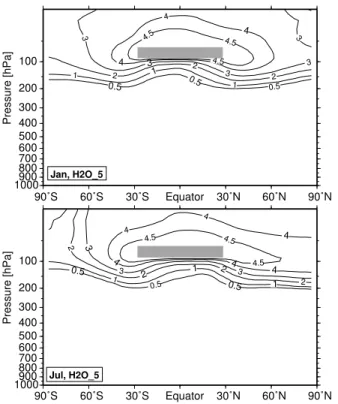
perturbation was set to+1 ppmv in the tropical lower stratosphere. Figure 5 shows the climatological mean distribution of the water vapor perturbation in H2O 5 for Jan-uary and July. The dark shaded area indicates the “source region” where the pertur-bation is fixed. Approximately 70% of the tropical perturpertur-bation can be found around 70◦N (∼3.5 ppmv), whereas the perturbation is much lower around 70◦S (southern

15

hemispheric values 15%–20% lower than northern hemispheric values). Again, these results indicate a more intense northward transport. The strong dehydration of the Antarctic winter stratosphere is clearly visible. The dehydration of the Arctic winter stratosphere is less intensive. The minimum values of the additional water vapor in the Antarctic winter stratosphere fall below 1 ppmv in H2O 5 (H2O 1: ∼0.1 ppmv),

20

whereas the minimum values in the Arctic winter stratosphere are around 3 ppmv in H2O 5 (H2O 1: ∼0.45 ppmv). The results for simulation H2O 1 show the same pattern, just the absolute values are 5 times smaller.

4. Results

As mentioned above, the oxidation of H₂O and CH₄ by O(1D) (Reaction R1 and R2) is the primary source of OH in the stratosphere. Excited oxygen atoms, O(1D), are produced by photolysis of O₃ at wavelengths shorter than about 320 nm. Associated

(12)

ACPD

tropical lowermost stratosphere is the region of the highest H₂O perturbation, the most pronounced changes of the OH distribution are expected for the tropical lowermost stratosphere within all perturbation scenarios. In turn, the production of H₂O by the methane oxidation is enhanced:

CH₄+ OH→ CHO2 ₃O₂+ H2O (R3)

The stratospheric OH increase causes a variety of changes concerning the different ozone production and destruction cycles. The results of our study will show that these changes yield to a net ozone destruction. At first a short overview concerning the role of OH within the stratospheric ozone chemistry is given. Different catalytic cycles take part in stratospheric ozone destruction. These cycles can be written in a general form:

X+ O3→ XO+ O2 XO+ O → X + O2

O₃+ O → O2+ O2 (R4)

where X can be one of the free radicals H, OH, NO, Cl or Br. Beside this general form additional catalytic cycles exist, but only an additional HO_x cycle is mentioned here:

OH+ O3→ HO₂+ O2 HO₂+ O₃→ OH+ O₂+ O₂

O₃+ O3→ O₂+ O2+ O2 (R5)

Of special interest for our study is the coupling of the HO_x and NO_x/ClO_x cycles, since coupling reactions change the catalytic effectiveness of the separate catalytic cycles. The coupling of the HO_xand NO_xcycles occurs by the following reactions:

(13)

ACPD

Print Version Interactive Discussion © EGU 2004 OH+ NO2+ M → HNO3+ M (R7) HNO₃→ OHhν + NO₂ (R8) HNO₃+ OH → H2O+ NO3 (R9)

An increase of OH should result in an enhanced transformation of NO₂ into the reser-voir species HNO₃. Since ReactionR9 is less effective in releasing NOx which is tied in the reservoir species HNO₃, the coupling of the HO_x and NO_x cycle is expected to reduce the catalytic effectiveness of the NO_xcycle. ReactionR6controls the partition-ing between OH and HO₂which is important for the effectiveness of the HOxcycle. As OH increases, ozone destruction by the ClO_xcycle becomes more effective:

OH+ HCl → H2O+ Cl (R10)

HO₂+ ClO → HOCl + O2 (R11)

The reservoir species HCl is converted back into active Cl by ReactionR10. Hypochlor-ous acid (HOCl) is photolyzed to OH and active Cl. Increasing stratospheric H₂O (and hence OH) decreases the catalytic effect of the NOx cycle and enhances the e ffec-tiveness of the ClO_x cycle and the HO_x cycle on the O₃ destruction. The following sections present a quantification of the impact of increasing stratospheric water vapor

5

on stratospheric chemistry.

4.1. Short-term increase of stratospheric water vapor

This section deals with the impact of a short-term increase of stratospheric water vapor as associated with strong volcanic eruptions like the Mount Pinatubo eruption in 1991 (simulation VOLC). It should be pronounced that the volcanic impact on stratospheric

10

aerosol is not considered in the simulations. Neither an enhanced ozone depletion caused by the increasing aerosol surface area nor the aerosol effect on the tropical tropopause temperature is taken into account. Figure6shows the percentage changes of the OH concentration at 50 hPa (upper panel) and 80 hPa (lower panel) in the VOLC

(14)

ACPD

hemispheres. The most pronounced changes occur within the tropics associated with the highest H₂O perturbation. The tropical OH increase peaks in July with up to+15% and more at 80 hPa and in August with up to 7% at 50 hPa. The 50 hPa level is above the “source” region of the H₂O perturbation (≈96–70 hPa). Thus, the upward transport

5

within the tropics takes about one month between 80 and 50 hPa. Of special interest are the two peaks at ca. ±30–40◦ at 80 hPa. This pattern is associated with the pol-wards and downpol-wards transport of the maximum OH signal. In contrast, at 50 hPa the maximum is located symmetrically around the equator. The percentage changes of the monthly and zonal mean OH concentration depending on the altitude for August are

10

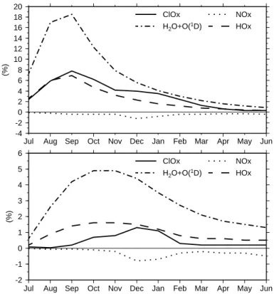
displayed in Fig.7. The downward transport at ca. ±30–40◦ is clearly visible in both hemispheres, but it is more pronounced in the southern hemisphere. The changes within the polar winter regions are not relevant due to the low OH background con-centrations. As mentioned above changing stratospheric OH levels affect the different ozone destruction reactions. Figure8shows the relative changes of the effectiveness

15

of the HO_x, ClO_x and NO_x cycle as well as of the reaction H₂O+ O(1D) → 2OH (re-moval of odd oxygen) at 50 hPa and different latitudes (upper panel: tropics, lower panel: mid-latitudes) caused by the stratospheric OH increase. The background con-tribution of the different processes to the ozone destruction in CNTL is given in the first row of Table4. The dominant effect is the increase of ozone destruction through the

20

HO_x cycle. Within the tropics the increase of the HO_x cycle peaks in September with approximately+7% compared to CNTL. Additionally, the ClOx cycle and the reaction H₂O+ O(1D) become more effective, but both ozone destroying reactions have only little importance in the tropics or mid-latitudes. The changes of the NO_xcycle are neg-ligible (≤−1%). Qualitatively, the mid-latitudes show the same results. The changes

25

of the effectiveness are less pronounced than in the tropics since the OH increase is less. Additionally, the peaks are slightly shifted to November/December because of the transport times between tropics and mid-latitudes.

(15)

ex-ACPD

short-term total ozone increase within the tropics during July is associated with an enhanced ozone production by the following reactions (enhanced NO₂photolysis):

HO₂+ NO → OH + NO2 (R12)

NO₂→ NOhν + O (R13)

O₂+ O → O3 (R14)

This increased ozone production is restricted to the altitude range 100–80 hPa and compensates the enhanced effectiveness of the HOx cycle. One month later the water vapor perturbation has also reached higher altitudes, where the ozone depletion by the HO_x cycle becomes more important. Then, the enhanced ozone destruction by the HO_x cycle dominates the increased ozone production at lower altitudes. Whether a

5

tropical water vapor perturbation leads to ozone loss or ozone production depends on the altitude.

No results are shown for southern high latitudes during Antarctic winter and spring in Fig.9. Numerical effects lead to an unrealistic increase of ClONO2 in the Antarctic stratosphere, resulting in a reduced ozone removal by the ClO_x cycle. The ClONO₂

10

increase occurs right after the start of the experiments. Dynamical reasons for this ClONO₂ increase are not possible, since the experiments CNTL and VOLC simulate identical meteorology. Chemical conversion between the individual members of the ClX-family caused by the OH increase is also very unlikely, since the changes of other chemical species like HCl or ClO_xdo not show an adequate behavior. Additionally, the

15

transport times between the tropical “source” region of the water vapor perturbation and the southern polar stratosphere are inappropriate to explain these rapid changes.

Interestingly, the most pronounced total column ozone reduction takes place at north-ern high latitudes during spring/early summer. Since the chemical ozone destruction is only slightly enhanced in VOLC during Arctic spring this result seems to be

associ-20

ated with the transport of air masses with reduced ozone content from the tropics to northern high latitudes during winter.Grewe et al.(2004) studied the large-scale

(16)

trans-ACPD

30 hPa with the climate-chemistry model E39/C. Low ozone air masses are transported from the tropics to higher latitudes by wave breaking events, so-called streamers. They showed that streamers cause a 30% (50%) decrease of ozone at the extra-tropical tropopause of the summer (winter) hemisphere.

5

The changes displayed in Fig. 9 are statistically significant although the changes are less than 1% of the total column ozone. For this study only the variability of the chemical signal and not the variability of the dynamical signal is used for the t-test since all simulations have an identical meteorology.

Unfortunately, no observational data are available for the period right after the Mount

10

Pinatubo eruption which would be suitable for a comparison with the model results. Following the volcanic eruption SAGE II (Stratospheric Aerosol and Gas Experiment) ozone values were being systematically overestimated caused by the Pinatubo aerosol. SAGE II ozone values below 22 km altitude are affected by aerosol for approximately 2 years after the Pinatubo eruption (SPARC,1998). HALOE (Halogen Occultation

Exper-15

iment) and MLS (Microwave Limb Sounder) satellite data are available since October 1991, i.d. no pre-Pinatubo observations are available for comparison.

4.2. Long-term increase of stratospheric water vapor

This section presents the impact of a long-term increase of stratospheric water va-por on the stratospheric chemistry as simulated in the model experiments H2O 1 and

20

H2O 5. Since the results of both experiments show the same patterns the follow-ing figures refer to the simulation H2O 5. Figure 10 shows the relative changes of OH in H2O 5 compared to the reference simulation CNTL. The zonal mean changes, averaged over 5 years, for July and January are displayed. As expected the strato-spheric OH content increases. The highest OH increase occurs in the tropical lower

25

stratosphere. An additional stratospheric water vapor content of+5 ppmv (+1 ppmv) results in a 50% (10%) increase in OH (≈+20×105−_+25×105 molecules/cm3, H2O 1:≈+5×105molecules/cm3). Thus, the OH response to increasing stratospheric

(17)

ACPD

the changes. Since the existence of OH is coupled to the sunlit atmosphere, OH back-ground concentrations are very low during the permanent polar night. Thus the high percentage changes in the winter polar hemispheres are negligible. In turn, the water vapor production by the oxidation of methane (ReactionR3) is up to 75% (10%) higher

5

in H2O 5 (H2O 1) than in CNTL (not shown). The regions of maximum increase in water vapor production are directly connected to the regions of highest OH increase.

Table4summarizes the changes of different ozone destroying cycles and reactions at 50 hPa and different latitudes caused by the H2O perturbation. The first row displays the contribution of the different ozone destroying reactions to the net ozone destruction

10

in the control simulation CNTL. The following two rows display the percentage changes in the perturbation experiments H2O 5 and H2O 1 compared to CNTL. The dominating effect is the enhanced effectiveness of the catalytic ozone removal by the HOx cycle (Reactions R4–R5). Within the tropics the effectiveness of the HOx cycle is 29.0% (6.4%) higher in H2O 5 (H2O 1) than in CNTL. The effectiveness of the HOx cycle

15

increases almost linear with rising OH concentrations. The changes of the NO_x cycle and the removal of excited oxygen by the reaction with water vapor also show a linear behavior with increasing OH. The last mentioned process plays only a minor role in the ozone destruction. In contrast, the ClO_x cycle shows a strong non-linear behavior. The ClO_x cycle is 7.8% more effective in H2O 1, but above 100% more effective in

20

H2O 5. However, the contribution of the ClO_xcycle in the tropics is very small. Within mid-latitudes the different ozone destruction cycles show qualitatively the same pattern except the ClO_x cycle which increases only slightly with increasing OH.

The increase in OH does not only affect ozone destruction, it also results in an en-hanced ozone production. For example, as stratospheric ozone declines, ultraviolet radiation penetrates deeper into the stratosphere which leads to an enhanced ozone production by the Chapman mechanism:

(18)

ACPD

O₂+ O + M → O₃+ M. (R16)

This process affects mainly the tropical lower stratosphere, but the ozone produc-tion by the Chapman mechanism is only slightly enhanced (less than 5% in H2O 5). Ozone production increases as well caused by the increased NO₂ concentration, HO₂+ NO → OH + NO2, which is photolyzed. Additionally, the methyl peroxy radi-cal CH₃O₂, a product of the methane oxidation (ReactionR3), reacts with NO to NO₂,

5

which again leads to an increased ozone production, but this process is two orders of magnitude less important than the other mentioned reactions. However, the increased ozone production can not compensate the enhanced ozone destruction. This effect was already mentioned in the previous section.

The above mentioned results deal with the gas-phase chemistry and do not con-sider possible effects on the heterogeneous reactions on polar stratospheric clouds (PSCs). PSCs occur between 10 and 25 km at temperatures below ≈190 K. Such low temperatures are more frequent in the Antarctic polar vortex. The release of active chlorine from the reservoir species HCl and ClONO₂ is very slow in the gas-phase. PSCs promote the activation of chlorine. At sunrise, activated chlorine compounds are easily photolyzed and catalytic ozone destruction starts. The chemistry module CHEM considers the following heterogeneous reactions on PSCs and sulfate aerosols:

HCl+ ClONO2→ Cl₂+ HNO3 (R17)

H₂O+ ClONO₂→ HOCl+ HNO₃ (R18)

HOCl+ HCl → Cl2+ H2O (R19)

N₂O₅+ H2O → 2HNO₃ (R20)

Table4displays the percentage changes of the different ozone destroying reactions

10

at 50 hPa in polar regions during spring. There is a remarkable interhemispheric dif-ference of the importance of the NO_xand ClO_xcycle. At the North Pole, the NO_xcycle dominates the ozone destruction, whereas the ClO_x cycle contributes nearly 90% to the ozone destruction at the South Pole which is associated with the strong denitrifica-tion of the Antarctic stratosphere during winter. The denitrificadenitrifica-tion removes NO_x from

(19)

ACPD

ozone destruction by the ClO_x cycle. The impact of increasing water vapor is more pronounced at the South Pole where ozone destruction in general (sum of all ozone destroying reactions/cycles) increases (Table4). The most important changes during Antarctic spring concern the NO_x and ClO_x cycle. The effectiveness of the ClOx cycle

5

is ≈50% higher in H2O 1 and 2.5 times higher in H2O 5. The additional water vapor leads to an increase of PSCs Type II (ice) within the Antarctic polar vortex which is obvious in the strong dehydration of the Antarctic winter stratosphere (Fig.5). In turn, the activation of chlorine from the reservoir species HCl and ClONO₂is enhanced. In contrast, the NO_xcycle becomes ≈50% less effective in H2O 1 and is almost vanished

10

in H2O 5. The additional stratospheric water vapor seems to have no impact on the heterogeneous chemistry in northern polar spring. The ozone destruction rate in gen-eral remains nearly unchanged, but the contribution of the different ozone destroying reactions is shifted (Table4).

As a result of the above mentioned processes the ozone concentration decreases

al-15

most everywhere. Figure11displays the ozone changes determined by the differences of the zonal mean climatological ozone volume mixing ratio between the simulations H2O 5 and CNTL for January and July. The strongest ozone reductions occur in the polar regions of both hemispheres. The maximum in the winter hemisphere is slightly shifted downwards compared to the summer hemisphere. Tropospheric changes do

20

not exceed more than −1%. The ozone decline in H2O 5 is ≈5 times higher than in H2O 1. The most pronounced ozone changes are computed in the southern hemi-sphere with values up to −10% (−3%) in the simulation H2O 5 (H2O 1). The change of total column ozone between the simulations H2O 5 and CNTL is presented in Fig.12. In the tropics and the northern the pattern is very uniform without any seasonal

vari-25

ability. As expected, the most pronounced changes of total column ozone occur during southern polar spring with values up to −15% (H2O 5) and −3% (H2O 1), respec-tively. The southern polar ozone decline is not statistically significant during Septem-ber/October and December/January (see also Fig.11). This feature is associated with

(20)

ACPD

cycle is especially pronounced in the southern hemisphere. Throughout the southern winter and springtime the content of the water vapor perturbation decreases rapidly to values less than 1 ppmv (H2O 5) and 0.1 ppmv (H2O 1), respectively. This de-hydration of the Antarctic winter lower stratosphere is associated with extremely low

5

temperatures. The duration as well as the beginning of the dehydration of the Antarctic winter lower stratosphere varies from year to year, resulting in a non-uniform ozone depletion pattern.

So far, this section dealt with the stratospheric changes caused by a water vapor in-crease. But as shown in Fig. 10 tropospheric OH concentrations increase slightly

10

as well. As stratospheric ozone decreases the absorption of short-wave radiation by ozone is reduced and the amount of short-wave radiation reaching the ground in-creases. In the troposphere the photolysis of ozone at wavelengths < 319 nm is crucial for the formation of OH (ReactionsR1–R2). Figure13 shows percentage changes of the surface dose at 309 nm in the simulation H2O 5 compared to CNTL. The amount

15

of short-wave radiation reaching the ground increases. The pattern shown in Fig.13is directly correlated to the ozone changes displayed in Fig.12: The percentage increase in surface dose is highest at southern high latitudes during southern spring when the total column ozone reduction is highest as well. In this region the surface dose in-crease at 309 nm is+50%. Within the tropics the surface dose is enhanced by +2%.

20

The surface dose changes in simulation H2O 1 show the same pattern (not shown), but the percentage changes are 5 times smaller than in H2O 5.

5. Conclusions

The impact of different idealized stratospheric water vapor perturbations on the strato-spheric ozone chemistry without any feedback on atmostrato-spheric dynamics was studied

25

with the coupled climate-chemistry model ECHAM4.L39(DLR)/CHEM. A long-term in-crease (+1 ppmv and +5 ppmv) as well as a short-term increase (“volcanic eruption”,

(21)

ACPD

impact of water vapor perturbations on the effectiveness of different ozone destroy-ing reactions as well as coupldestroy-ing effects between different chemical processes were detailed analyzed.

A stratospheric water vapor increase leads to an increased OH concentration which

5

results primarily in an enhanced ozone depletion by the HO_x-cycle. The coupling of the HO_x-cycle with the NO_x- and ClO_x-cycle leads to a less effective NOx-cycle and a slightly enhanced effectiveness of the ClOx-cycle. A long-term increase in strato-spheric water vapor affects the heterogeneous ozone destruction (ClOx-cycle) within the Antarctic polar vortex caused by an enhanced formation of PSCs Type II (ice).

Het-10

erogeneous ozone chemistry in the Arctic polar vortex is not affected. The simulated short-term perturbation does not affect heterogeneous ozone chemistry.

A comparison between the short-term (VOLC) and long-term water vapor perturba-tions (H2O 1 and H2O 5) reveals some differences. VOLC shows an increase in total column ozone in the tropics during July and August. During this period of the simulation

15

VOLC the water vapor perturbation is not yet evenly distributed and the OH increase is concentrated on the lowermost stratosphere. The ozone chemistry is dominated by the ozone production caused by an enhanced NO₂photolysis (ReactionsR12–R14). The HO_x cycle becomes more important in higher altitudes. The simulations H2O 1 and H2O 5 do not show a similar effect since the water vapor perturbation has reached a

20

steady distribution. Simulation VOLC as well as simulation H2O 1 show a 7% increase in OH at 50 hPa within the tropics during August. Despite similar water vapor and OH perturbations VOLC and H2O 1 show different ozone changes within this region. The ozone reduction in H2O 1 amounts −1%, but only −0.07% in VOLC. At this alti-tude the ozone concentration is dynamically controlled (WMO,1986). Thus, the effect

25

of a short-term change in chemistry is less important than the impact of a long-term change resulting in different ozone transport.

The almost negligible impact of the short-term water vapor changes on tropical to-tal ozone columns can therefore not explain the ozone decline in the transient model

(22)

ACPD

the stratosphere and amplifies tropical ascent by roughly 20%, leading to an additional uplift during a volcanic period of roughly 1.2 km, which compares reasonably with the uplift of the Pinatubo aerosol cloud by 1.8 km (DeFoor et al.,1992;Kinne et al.,1992). Applying a linearized transport-chemistry column model and using E39/C values for

5

uplift, ozone production and destruction rates of ozone, the simulated vertical ozone profile can be reproduced within 5 to 25% accuracy. Introducing an additional uplift of 1.2 km over 8 months produces a vertical displacement of the ozone profile and a re-duction of the ozone column of 5% (red stars in Fig.2b), agreeing well with the findings ofKinne et al. (1992). This means that the ozone decline simulated during volcanic

10

eruptions is dominated by dynamic effects.

WithinIPCC (1999) the effects of a future (year 2015) supersonic aircraft fleet (500 aircraft) on stratospheric O₃, H₂O and other species was conducted with various 2-D and 3-D CTMs (chemistry transport models). The maximum H₂O perturbations caused by supersonic aircraft emissions occur in the northern hemisphere lower stratosphere

15

(≈20 km) and range from 0.4 ppmv to 0.7 ppmv. The percentage changes in to-tal column ozone averaged over the northern hemisphere are in the −0.3. . .−0.6% range. This scenario includes only H₂O emissions, NO_x emissions have been ex-cluded (EI(NO_x)=0). Performing further scenarios with different EI(NO_x) all models predicted that the most significant supersonic impact on ozone is caused by the water

20

vapor emissions and that the addition of NO_x emissions leads to a less ozone deple-tion (IPCC,1999). The water vapor perturbation in H2O 1 in the northern hemisphere lower stratosphere (≈50 hPa) range from 0.5 ppmv to 0.8 ppmv, depending on season (Fig.5). The total ozone depletion averaged over the northern hemisphere is ≈−0.5% in H20 1. In this respect the results of H20 1 are within the range ofIPCC(1999).

25

Figure14shows the total column ozone decrease for different geographical regions for simulation H2O 1 and H2O 5. In agreement with the above mentioned results the ozone response to the stratospheric water vapor increase is almost linear. Taking into account the simulated water vapor increase of +0.029 ppmv/yr between 1980 and

(23)

ACPD

approximately+0.6 ppmv. According to the linear behavior of the ozone response, at least on hemispheric scales, a perturbation of+0.6 ppmv leads to a global total col-umn ozone reduction of −0.5% (indicated by the vertical dash-dotted line in Fig.14). The simulated ozone decline between 1980 and 2000 amounts −3.4%, considering

5

the increasing chlorine loading and climate change. Thus the stratospheric water va-por increase plays a significant role in ozone decline. Dvortsov and Solomon(2001) analyzed the response of stratospheric temperatures and ozone to past (+1%/yr) and future increases in stratospheric humidity with a 2-D radiative-chemical-dynamical model. Their results show an additional depletion of mid-latitude column ozone of

10

−0.3%/decade caused by the stratospheric water vapor increase. So our results are in good agreement with the findings ofDvortsov and Solomon (2001). A prolonged increase in stratospheric water vapor could have a significant effect on stratospheric ozone depletion: the chemical effect of the water vapor increase and the cooling effect on stratospheric temperatures together lead to a further ozone depletion, which could

15

delay the ozone recovery caused by the expected future reduction of the stratospheric chlorine loading (Shindell et al.,1998).

Acknowledgements. This study was partly funded by the EU project SCENIC. The model

sim-ulations have been performed on the NEC SX-6 high performance computer of the German Climate Computing Centre (DKRZ), Hamburg. We thank M. Ponater for his helpful answers

20

concerning the “last secrets” of the model ECHAM4.L39(DLR)/CHEM.

References

Bates, D. R. and Nicolet, M.: The photochemistry of atmospheric water vapor, J. Geophys. Res., 55, 301–327, 1950. 6561

Benkovitz, C. M., Scholtz, M. T., Pacyna, J., Tarrason, L., Dignon, J., Voldner, E. C., Spiro, P. A.,

25

Logan, J. A., and Graedel, T. E.: Global gridded inventories of anthropogenic emissions of sulfur and nitrogen, J. Geophys. Res., 101, 29 239–29 253, 1996. 6587

(24)

ACPD

stratospheric aircraft: Report of the 1992 models and measurement workshop, edited by M. Prather and E. Remsberg, NASA Reference Publ. 1292, pp. 703–706, Washington, DC, 1993. 6564

Considine, D. B., Rosenfield, J. E., and Fleming, E. L.: An interactive model study of the

influ-5

ence of the Mount Pinatubo aerosol on stratospheric methane and water trends, J. Geophys. Res., 106, 27 711–27 727, 2001. 6563

DeFoor, T. E., Robinson, E., and Ryan, S.: Early lidar observations of the June ’91 Pinatubo eruption plume at Mauna Loa Observatory, Hawaii, Geophys. Res. Lett., 19, 187–190, 1992.

6579 10

Dvortsov, V. L. and Solomon, S.: Response of the stratospheric temperatures and ozone to past and future increases in stratospheric humidity, J. Geophys. Res., 106, 7505–7514, 2001.

6562,6580

Evans, S. J., Toumi, R., Harries, J. E., Chipperfield, M. P., and Russell III, J. M.: Trends in the Stratospheric Humidity and the Sensitivity of Ozone to these Trends, J. Geophys. Res., 103,

15

8715–8725, 1998. 6561,6562

Fioletov, V. E., Bodeker, G. E., Miller, A. J., McPeters, R. D., and Stolarski, R.: Global and zonal total ozone variations estimated from ground-based and satellite measurements: 1964– 2000, J. Geophys. Res., 107, 4647, doi:10.1029/2001JD001350, 2002. 6590

Gauss, M., Isaksen, I. S. A., Wong, S., and Wang, W.-C.: Impact of H₂O emissions

20

from cryoplanes and kerosene aircraft on the atmosphere, J. Geophys. Res., 4304, doi:10.1029/2002JD002623, 2003. 6563

Glaze, L., Baloga, S. M., and Wilson, L.: Transport of atmospheric water vapor by volcanic eruption columns, J. Geophys. Res., 102, 6099–6108, 1997. 6562

Grewe, V., Brunner, D., Dameris, M., Grenfell, J. L., Hein, R., Shindell, D., and Staehelin,

25

J.: Origin and variability of upper tropospheric nitrogen oxides and ozone at northern mid-latitudes, Atmos. Environ., 35, 3421–3433, 2001. 6564,6587

Grewe, V., Shindell, D. T., and Eyring, V.: The impact of horizontal transport on the chemical composition in the tropopause region: Lightning NOx and streamers, Advances in Space Research, 33, 1058–1061, 2004. 6568,6572

30

Hanisco, T. F., Lanzendorf, E. J., Wennberg, P. O., Perkins, K. K., Stimpfle, R. M., Voss, P. B., Anderson, J. G., Cohen, R. C., Fahey, D. W., Gao, R. S., Hintsa, E. J., Salawitch, R. J., Margitan, J. J., McElroy, C. T., and Midwinter, C.: Sources, sinks and the distribution of OH

(25)

ACPD

Hao, W. M., Liu, M.-H., and Crutzen, P. J.: Estimates of annual and regional releases of CO₂ and other trace gases to the atmosphere from fires in the tropics, based on the FAO statistics for the period 1975–1980, Vol. 84 of Fire in the Tropical Biota, Ecological Studies, pp. 440– 462, Springer-Verlag, New York, 1990. 6587

5

Hein, R., Dameris, M., Schnadt, C., Land, C., Grewe, V., K ¨ohler, I., Ponater, M., Sausen, R., Steil, B., Landgraf, J., and Br ¨uhl, C.: Results of an interactively coupled atmospheric chemistry–general circulation model: comparison with oberservations, Ann. Geophys., 19, 435–457, 2001,

SRef-ID: 1432-0576/ag/2001-19-435. 6562,6564,6565 10

IPCC: Aviation and the global atmosphere, p. 373, Intergovernmental Panel on Climate Change, Cambridge University Press, Cambridge, UK, 1999. 6563,6579

IPCC: Climate Change 2001 – The scientific basis, p. 881, Intergovernmental Panel on Climate Change, Cambridge University Press, New York, USA, 2001. 6564,6586,6587

Kinne, S., Toon, O. B., and Prather, M. J.: Buffering of stratospheric circulation by changing

15

amounts of tropical ozone – a Pinatubo case study, Geophys. Res. Lett., 19, 1927–1930, 1992. 6579

Land, C., Ponater, M., Sausen, R., and Roeckner, E.: The ECHAM4.L39(DLR) atmosphere GCM — Technical description and model climatology, DLR Forschungsbericht 1999-31, ISSN 1434-8454, K ¨oln, 1999. 6564

20

Lawrence, M. G., J ¨ockel, P., and von Kuhlmann, R.: What does the global mean OH concen-tration tell us?, Atmos. Chem. Phys., 1, 37–49, 2001,

SRef-ID: 1680-7324/acp/2001-1-37. 6565

Michelsen, H. A., Irion, F. W., Manney, G. L., Toon, G. C., and Gunson, M. R.: Features and trends in Atmospheric Trace Molecule Spectroscopy (ATMOS) version 3 stratospheric water

25

vapor and methane measurements, J. Geophys. Res., 105, 22 713–22 724, 2000. 6561

Morris, G. A., Rosenfield, J. E., Schoeberl, M. R., and Jackman, C. H.: Potential impact of subsonic and supersonic aircraft exhaust on water vapor in the lower stratosphere assessed via a trajectory model, J. Geophys. Res., 4103, doi:10.1029/2002JD002614, 2003. 6563

Nedoluha, G. E., Bevilacqua, R. M., Gomez, R. M., Siskind, D. E., Hicks, B. C., Russell III, J. M.,

30

and Connor, B. J.: Increases in middle atmospheric water vapor as observed by the Halogen Occultation Experiment and the ground-based Water Vapor Millimeter-wave Spectrometer from 1991 to 1997, J. Geophys. Res., 103, 3531–3543, 1998. 6561

(26)

ACPD

strato-spheric water vapor from balloonborne frostpoint hygrometer measurements at Washington D.C., and Boulder, Colorado, Geophys. Res. Lett., 27, 3453–3456, 2000. 6561,6562,6589

Roeckner, E., Arpe, K., Bengtsson, L., Christoph, M., Claussen, M., D ¨umenil, L., Esch, M., Giorgetta, M., Schlese, U., and Schulzweida, U.: The atmospheric general circulation model

5

ECHAM–4: Model description and simulation of present–day climate, Report No. 218, Max-Planck-Institut f ¨ur Meteorologie, Hamburg, 1996. 6564

Rosenlof, K. H.: Transport changes inferred from HALOE water and methane measurements, J. Met. Soc. Jap., 80, 831–848, 2002. 6561

Rosenlof, K. H., Oltmans, S. J., Kley, D., Russell III, J. M., Chiou, E.-W., Chu, W. P., Johnson,

10

D. G., Kelly, K. K., Michelsen, H. A., Nedoluha, G. E., Remsberg, E. E., Toon, G. C., and McCormick, M. P.: Stratospheric water vapor increases over the past half-century, Geophys. Res. Lett., 28, 1195–1198, 2001. 6561

Schmitt, A. and Brunner, D.: Emissions from aviation and their development over time, in Pollu-tants from air traffic – results of atmospheric research 1992–1997, edited by: Schumann, U.,

15

Chloud, A., Ebel, A., K ¨archer, B., Pak, H., Schlager, H., Schmitt, A., and Wendling, P., Vol. 97-04 of DLR-Mitt., 37–52, DLR K ¨oln, Germany, 1997. 6587

Shindell, D. T., Rind, D., and Lonergan, P.: Increased polar stratospheric ozone losses and delayed eventual recovery owing to increasing greenhouse-gas concentrations, Nature, 392, 589–592, 1998. 6580

20

SPARC: SPARC/IOC/GAW Assessment of trends in the vertical distribution of ozone, SPARC Report #1, WMO Ozone Research and Monitoring Project Report #43, 1998. 6573

Spivakovsky, C. M., Logan, J. A., Montzka, S. A., Balkanski, Y. J., Foreman-Fowler, M., Jones, D. B. A., Horowitz, L. W., Fusco, A. C., Brenninkmeijer, C. A. M., Prather, M. J., Wofsy, S. C., and McElroy, M. B.: Three-dimensional climatological distribution of tropospheric OH:

25

Update and evaluation, J. Geophys. Res., 105, 8931–8980, 2000. 6565

Steil, B., Dameris, M., Br ¨uhl, C., Crutzen, P. J., Grewe, V., Ponater, M., and Sausen, R.: De-velopment of a chemistry module for GCMs: first results of a multiannual integration, Ann. Geophys., 16, 205–228, 1998,

SRef-ID: 1432-0576/ag/1998-16-205. 6564 30

Stenchikov, G. L., Kirchner, I., Robock, A., Graf, H.-F., Antu ˜na, J. C., Grainger, R. G., Lambert, A., and Thomason, L.: Radiative forcing from the 1991 Mount Pinatubo volcanic eruption, J. Geophys. Res., 103, 13 837–13 857, 1998. 6562

(27)

ACPD

J. G.: In-situ measurements of OH and HO₂ in the upper troposphere and stratosphere, J. Atmos. Sci., 52, 3413–3420, 1995. 6565

WMO: Atmospheric Ozone 1985: Global ozone research and monitoring report, Report No. 16, World Meteorological Organization, Geneva, 1986. 6578

5

WMO: Scientific assessment of ozone depletion: 2002, Report No. 47, World Meteorological Organization, Geneva, 2002. 6562

Yienger, J. J. and Levy, H.: Empirical model of global soil-biogenic NOxemissions, J. Geophys. Res., 100, 11 447–11 464, 1995. 6587

Zhou, X., Geller, M. A., and Zhang, M.: Cooling Trend of the Tropical Cold Point Tropopause Temperatures and its Implications, J. Geophys. Res., 106, 1511–1522, 2001. 6561

(28)

ACPD

Table 1. Overview of analyzed model experiments.

EXP feedback mode H₂O perturbation simulation period CNTL without feedback 0 ppmv, reference simulation 11 years

VOLC without feedback 2 ppmv, July and August, short-term increase 5 annual cycles July-June (last 5 years of CNTL) H2O 1 without feedback 1 ppmv, long-term increase 11 years

(29)

ACPD

Table 2. Mixing ratios of greenhouse gases adopted for the year 2000 as recommended by

IPCC(2001).

CO₂(ppmv) CH₄(ppmv) N₂O (ppbv) Cl_y(ppbv)

(30)

ACPD

Table 3. NO_x emissions adopted for the year 2000 (∗taking into accountIPCC(2001) rates of increase).

NO_xsource Global source (Tg(N)/yr) Reference

Air traffic 0.7 Schmitt and Brunner(1997)∗ Lightning ∼5 Grewe et al.(2001)

Industry, Traffic 33.0 Benkovitz et al.(1996)∗ Soils 5.6 Yienger and Levy(1995)∗ Biomass burning 7.1 Hao et al.(1990)∗

(31)

ACPD

Table 4. Ozone destroying cycles/reactions at 50 hPa, different latitudes and seasons. CNTL:

Contribution of each reaction to the total ozone destruction [%]. VOLC, H2O 1 and H2O 5: Changes compared to CNTL [%]. The term O₃-Loss includes all ozone destroying reactions considered in E39/C.

Annual Mean, Tropics Annual Mean, Mid-Latitudes O3-Loss HOx NOx ClOx H2O+ O( 1 D) O3-Loss HOx NOx ClOx H2O+ O( 1 D) CNTL – 77.1 14.0 1.4 2.9 – 60.8 19.6 8.4 1.4 H2O 1 +5.1 +6.4 −1.6 +7.8 +17.0 +2.4 +4.1 -2.2 +2.7 +12.7 H2O 5 +25.8 +29.0 −7.7 +114.9 +86.0 +11.0 +19.0 −7.0 +3.4 +64.0 VOLC (Aug) +5.0 +6.0 −0.2 +5.9 +17.0 +0.6 +0.9 -0.07 +0.03 +2.6 VOLC (Dec) +1.8 +2.3 −1.2 +4.0 +5.6 +0.9 +1.5 −0.8 +1.3 +4.4

Arctic Spring, Polar Regions Antarctic Spring, Polar Regions O3-Loss HOx NOx ClOx H2O+ O( 1 D) O3-Loss HOx NOx ClOx H2O+ O( 1 D) CNTL – 26.8 47.7 7.9 0.3 – 6.7 4.0 88.7 0.07 H2O 1 −0.9 +5.6 −6.7 +12.4 +10.5 +38.9 −3.4 -47.4 +46.4 +4.3 H2O 5 −1.5 +23.3 −17.5 +16.5 +55.7 +126.6 −22.8 −94.9 +149.1 +35.9

(32)

ACPD

1980 1982 1984 1986 1988 1990 1992 1994 1996 1998 2000

Water vapor mixing ratio

8

2 6

4

Fig. 1. Time series of individual water vapor soundings with the CMDL frostpoint

hygrom-eter between 24 and 26 km at Boulder, CO (black) (Oltmans et al., 2000), and of monthly mean water vapor mixing ratios from ECHAM4.L39(DLR)/CHEM at 40◦N, 20 hPa (red). The linear trend with the 95% confidence interval is 0.044±0.012 ppmv/yr for Boulder and 0.029±0.007 ppmv/yr for the model simulation. The dashed line indicates enhanced water vapor mixing ratios over Boulder in 1992 after the Pinatubo eruption.

(33)

ACPD

ozone column deviations (%)

(a) −36 −30 −24 −18 −12 −6 0 6 12 18 24 30 36 month −6 −4 −2 0 2

ozone column deviations (%)

(b)

Fig. 2. (a) Modeled total ozone deviations, deseasonalized with respect to the period 1979–

1987 and expressed as percentages of the ground-based time average for the period 1964-1980, area-weighted mean 90◦N–90◦S (seeFioletov et al.(2002) for details of analysis). Red line shows a 13-month running mean. (b) Modeled total ozone deviations within the tropics

(10◦N–10◦S) averaged over the last three major volcanic eruptions, expressed as percentages of the average for the period 1964–1980. Month 0 indicates the minimum ozone value after the volcanic eruptions. The eruptions occurred between 8 and 23 months earlier. The red stars indicate the estimated reduction of the ozone column caused by the additional uplift during a volcanic period applying a linearized transport-chemistry column model.