Stratospheric aerosol measurements by dual polarisation lidar

(1)

HAL Id: hal-00301445

https://hal.archives-ouvertes.fr/hal-00301445

Submitted on 29 Sep 2004

HAL is a multi-disciplinary open access

archive for the deposit and dissemination of sci-entific research documents, whether they are pub-lished or not. The documents may come from teaching and research institutions in France or abroad, or from public or private research centers.

L’archive ouverte pluridisciplinaire HAL, est destinée au dépôt et à la diffusion de documents scientifiques de niveau recherche, publiés ou non, émanant des établissements d’enseignement et de recherche français ou étrangers, des laboratoires publics ou privés.

Stratospheric aerosol measurements by dual polarisation

lidar

G. Vaughan, D. P. Wareing

To cite this version:

G. Vaughan, D. P. Wareing. Stratospheric aerosol measurements by dual polarisation lidar. Atmo-spheric Chemistry and Physics Discussions, European Geosciences Union, 2004, 4 (5), pp.6107-6126. �hal-00301445�

(2)

ACPD

4, 6107–6126, 2004

Stratospheric aerosol measurements by dual polarisation lidar

G. Vaughan and D. P. Wareing Title Page Abstract Introduction Conclusions References Tables Figures J I J I Back Close

Full Screen / Esc

Print Version

Interactive Discussion

Atmos. Chem. Phys. Discuss., 4, 6107–6126, 2004 www.atmos-chem-phys.org/acpd/4/6107/

SRef-ID: 1680-7375/acpd/2004-4-6107 © European Geosciences Union 2004

Atmospheric Chemistry and Physics Discussions

Stratospheric aerosol measurements by

dual polarisation lidar

G. Vaughan and D. P. Wareing

University of Wales, Aberystwyth, UK

Received: 22 July 2004 – Accepted: 8 September 2004 – Published: 29 September 2004 Correspondence to: G. Vaughan (gxv@aber.ac.uk)

(3)

ACPD

4, 6107–6126, 2004

Full Screen / Esc

Print Version

Abstract

We present measurements of stratospheric aerosol made at Aberystwyth, UK (52.4◦N, 4.06◦W) during periods of background aerosol conditions. The measurements were made with a lidar system based on a 532 nm laser and two polarisation channels in the receiver. When stratospheric aerosol amounts are very small, as at present,

5

this method is, potentially, free of a number of systematic errors that bedevil more commonly-used methods. The method rests on the assumption that the aerosol con-sists of spherical droplets which do not depolarise the lidar signal, which is valid un-der most conditions. Maximum lidar ratios in background aerosol of 1.03–1.06 were measured during the period 2001–2004, with integrated backscatter in the range

10

2–7×10−5sr−1. In January 2003, depolarising aerosol was measured, which in-validated the dual-polarisation measurements. On 10–11 January, the depolarising aerosol was clearly a polar stratospheric cloud (the first lidar observations of such clouds in the British Isles) but the aerosol observed on 7–8 January was too low in altitude and too warm to be a PSC.

15

1. Introduction

Since the decay of the aerosol cloud from Mt. Pinatubo there have been no major vol-canic eruptions disrupting the stratosphere, and the aerosol layer has decreased to very low optical depth (J ¨ager, 2001). Measuring the thickness of such a thin cloud ac-curately is not easy with a visible-wavelength lidar. The standard method for retrieval

20

of lidar data involves taking the ratio between the measured (elastic) lidar signal and a synthetic backscatter profile calculated from an assumed profile of temperature and ozone. This works well when there is plenty of aerosol (Thomas et al., 1987; Vaughan et al., 1994) but the inevitable uncertainty in the background profile introduces signif-icant systematic errors for very low aerosol amounts which are very difficult to

quan-25

(4)

ACPD

4, 6107–6126, 2004

Full Screen / Esc

Print Version

a Raman channel to observe scattering directly from N₂. Because of the wavelength shift this method is not free of assumptions about the atmospheric density profile, and suffers further because the very weak Raman signals limit the vertical extent of the signals. This can be overcome by measuring the air scattering profile with a polariser, which typically gives about ten times more signal than Raman. The basic principle is

5

that air depolarises the lidar signal slightly whereas spherical liquid aerosol does not. Thus, measuring the backscattered signals polarised parallel and perpendicular to the laser beam gives a measure of the total backscatter and that due to air alone, which can readily be combined to give the lidar backscatter ratio.

Beyerle (2000) gives a detailed critique of the polarisation lidar technique,

empha-10

sising that it is only suitable for low aerosol loadings but that under those conditions it can be superior to the standard or Raman techniques. One snag with the method is that it relies on very good polarisation of the laser and very little breakthrough in the receiver between the two polarisations, since the scattered signal perpendicular to the laser beam is only about 1% of the signal scattered parallel to it. Here we present

15

measurements of background aerosol using a polarisation lidar at Aberystwyth, UK (52.4◦N, 4.06◦N), using a calibration procedure to measure the breakthrough to 10%. The results are consistent with J ¨ager’s measurements of integrated backscatter, but this method can also distinguish very clearly between background aerosol and aerosol perturbed by a polarising component from volcanic ejecta or polar stratospheric clouds.

20

2. Experimental details

The lidar used in this study is essentially the same one as used in Vaughan et al. (1994). It uses a Nd-YAG laser at 532 nm as the source (300 mJ pulses at 10 Hz rep rate), giving a highly polarised laser beam. A 10× expanding telescope transmits this to the atmosphere. The system is biaxial, with complete overlap between receiver and

25

transmitter above 4 km. The receiver consists of a 60 cm parabolic mirror which, with a secondary, produces an f/4 beam brought to a focus at a field stop aperture above the

(5)

ACPD

4, 6107–6126, 2004

Full Screen / Esc

Print Version

centre of the mirror. Beyond this a prism rotates the beam through 90◦, which is col-limated before being directed through an interference filter onto a plain glass slide as a beamsplitter. The interference filter has a HPBW of 10 nm. Polarisers (Melles Griot dichroic sheet type) are placed directly before the photomultiplier tubes (EMI 9902KA) which detect the light. According to manufacturers’ data, the polarisers attenuate the

5

cross-polarised component by a factor of 105compared to the parallel-polarised com-ponent. Photon-counting electronics (Ortec MCS-PCI cards with ORTEC 935 constant fraction discriminators) complete the assembly.

Measurement runs are taken with 5000 laser shots (∼8 min) at a vertical resolution of 30 m. Because of the faint signals on the perpendicular channel many hours’ data need

10

to be collected to provide sufficient precision for analysis. In practice, a whole night’s observations are combined (the background being far too high for daytime operation). At the lower levels signal overload renders the measurements unreliable below 7 km; a correction for pulse pile-up is used for count-rates up to 20 MHz (S=S₀/(1−S₀τ) where

S₀ is the measured count rate, S the corrected count rate and τ the deadtime of 10 ns

15

set in the discriminator).

3. Data analysis and calibration

In principle the polarisation method is simple: coincident measurements are made of the backscattered signal parallel to the laser beam, S||, and that perpendicular to it, S⊥. It is assumed that there is no aerosol in a particular region of the atmosphere,

20

which provides a reference value to which the rest of the profile is normalised. It is also assumed that the aerosol does not depolarise the laser beam, whence the normalised ratio directly gives the lidar backscatter ratio R.

Allowance must be made for cross-talk between the two channels. This can arise from the laser not being perfectly polarised, depolarisation by the receiver optics, or

25

transmission of the unwanted beam by the polarisers. In practice, because S||S⊥, this is only important for breakthrough of the parallel component on the perpendicular

(6)

ACPD

4, 6107–6126, 2004

Full Screen / Esc

Print Version

channel. To determine this crosstalk, first of all the ratio of signals is measured with both polarisers set to pass S||. Let this ratio be K (in practice 0.03 with the present system). This is different to the reflectivity of the beamsplitter b||because of differences in the sensitivity of the two receiver channels. We take the values of b||and b⊥ as 0.02 and 0.19 respectively, appropriate to a crown glass beamsplitter.

5

We can express the ratio of signals S||/ S⊥ as follows:

S|| S⊥ = ξ

(1 − x)b||F||+ xb⊥F⊥

(1 − x)(1 − b⊥)F⊥+ x(1 − b||)F|| , (1)

where ξ is a system constant, F represents the flux of radiation back from the atmo-sphere and x is the instrumental depolarisation – the fraction of the “wrong” polarisation measured on each channel. Writing Eq. (1) for the case when both polarisers are set

10

to parallel (i.e. ratio of signals=K) and substituting for ξ we find:

S|| S⊥ = K (1 − x)F||+ xb⊥ b||F ⊥ (1 − x)(1−b⊥) (1−b||)F ⊥_{+ xF}||. (2)

In this derivation depolarisation of the laser beam is included implicitly, because its effect in practice is simply to increase the value of x. Thus F can be simply related to the backscatter coefficients of the atmosphere as

15

F||,⊥ ∝ β_M||,⊥+ β_A||,⊥, (3)

where subscript M denotes molecular (Rayleigh) scattering and A denotes aerosol scattering. Here we assume that β_A⊥=0, i.e. the aerosol is in the form of liquid droplets which do not depolarise.

Now x1 and F⊥F||. Omitting second-order terms in Eq. (2) and writing

(7)

ACPD

4, 6107–6126, 2004

Full Screen / Esc

Print Version Interactive Discussion © EGU 2004 (1−b)=(1−b⊥)/(1−b||), we find: S|| S⊥ = K (1 − x)(β||_M+ β_A||) (1 − x)(1 − b)β_M⊥ + x(β||_M+ β_A||) . (4)

The quantity (β||_M+β||_A)/β_M|| is effectively the lidar backscatter ratio R, so Eq. (4) simpli-fies to: S|| S⊥ = K (1 − x)R (1 − x)(1 − b)δ+ xR , (5) 5

where δ is the depolarisation due to air, β_M⊥/β||_M. For the present system we take this to be 0.0142 (Cairo et al., 1999), reduced by 5% to allow for the transmission of the rotational Raman lines through the interference filter (most of the depolarisation due to air is in fact due to rotational Raman scattering). The 5% figure was calculated from the measured filter transmission profile and a model of the rotational Raman spectrum

10

at stratospheric temperatures (Vaughan et al., 1993). Writing y=x/(1−x) this further simplifies to:

S|| S⊥ = K

R

δ(1 − b)+ yR . (6)

We now assume that there is a height in the atmosphere where no aerosol is present (either above 28 km or in the mid-troposphere, as shown below). The ratio of signals is

15

then due only to air, and the value of R is identically 1. Then

S|| S⊥ ! ref = K δ(1 − b)+ y (7)

(8)

ACPD

4, 6107–6126, 2004

Full Screen / Esc

Print Version

from which y may be determined. Dividing Eq. (6) by Eq. (7), and writing R_M for the measured value of R before taking system depolarisation into account, i.e. the nor-malised ratio of parallel to perpendicular signals:

R_M = R δ(1 − b)+ y δ(1 − b)+ yR =

R

1+_δ(1−b)(R−1)y_+y

. (8)

Inverting Eq. (8) we find:

5

R= RM

1 − (R_M− 1)y_δ (9)

with the obvious caveat that this equation applies only when R-1 is small (<0.1). For this system y was found to be 0.4±0.1%. Tests were also done with a narrow-band filter passing only the Cabannes (elastic) backscatter, which gave the same value of y but with a smaller error bar (0.04%). This value has been adopted for the results

10

presented here.

4. Results

4.1. Measurements of background aerosol

As mentioned above, the aerosol signal is faint compared to the molecular backscatter and lidar returns over a whole night have to be combined to get sufficient

signal-to-15

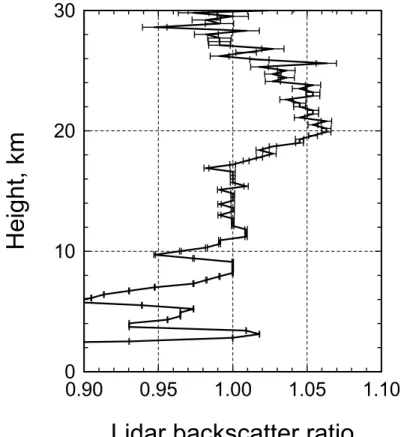
noise. This in turn means that measurements are effectively confined to clear nights in winter – not an especially frequent occurrence at Aberystwyth. An example from the night of 11 to 12 December 2001 is shown in Fig. 2. The profile has been normalised at 8 km because the signal at the top of the profile was too noisy; this introduces an uncertainty of ∼0.01 to the peak value of R. Below 8 km cirrus cloud and counter

over-20

load render the measurements unreliable. The profile shows almost no aerosol up to 17 km, with a increase to a peak value of 1.065 at 20 km.

(9)

ACPD

4, 6107–6126, 2004

Full Screen / Esc

Print Version

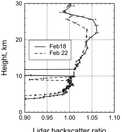
The second examples are from 18 and 22 February 2004 (Fig. 3). Here the profiles have been normalised to the ratio at 30 km, but they show that the mid-troposphere is aerosol-free (some cirrus affects the measurements on both days). The aerosol layer now extends lower than in December 2001 and, interestingly, extends higher on 18 February than on 22 February. The latter profile was taken in a more polar airmass

5

than the former, which indicates that the polar air contained less background aerosol than the midlatitude air.

In all, in the period April 2001–February 2004 sixteen nights’ data were obtained with the lidar; data are summarised in Table 1. The maximum lidar ratio in these profiles varied between 1.03 and 1.06, with the exception of January 2003 which is discussed

10

below. Much of this variation can be accounted for by the statistical uncertainty in fitting the profiles above the aerosol layer. The integrated backscatter from these profiles (cal-culated using the CIRA standard atmosphere) was in the range 2–7×10−5sr−1. This is in agreement with J ¨ager et al. (2001), and using a ratio of extinction to backscat-ter appropriate to post-Pinatubo aerosol of 50 sr (J ¨ager and Deshler, 2002, 2003) it

15

corresponds to an optical depth of 1–3.5×10−3. 4.2. Depolarising aerosol

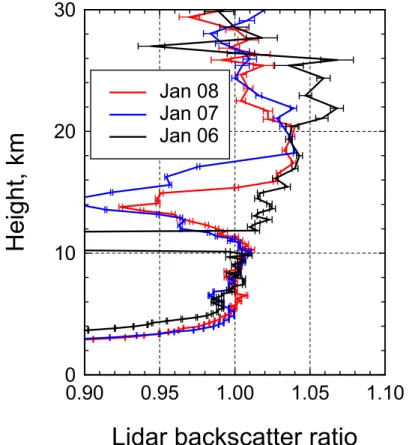
On most occasions the assumption that the aerosol does not depolarise appeared valid. However, this was not always the case. On 7/8 January and 8/9 January 2003 profiles were measured with a clear layer of depolarising particles in the lower

strato-20

sphere (Fig. 4). The ratio R was now <1 between 11 and 15.5 km, showing the pres-ence of depolarising aerosol. Near 20 km, the lidar backscatter ratio of 1.04 was con-sistent with the profiles measured on 6/7 January. During this period, the polar vortex was approaching Aberystwyth, and indeed reached it on 10 January (see below). The greater amount of aerosol above 20 km on 6/7 January is therefore consistent with the

25

observations of February 2004, since it corresponds to a less polar air mass.

To demonstrate that the depolarising aerosol are real (rather than an instrument mal-function), the data for the 8/9 January were also analysed using the “standard method”

(10)

ACPD

4, 6107–6126, 2004

Full Screen / Esc

Print Version

of taking the ratio to a synthetic density profile. This profile was generated from the ra-diosonde ascent at 00:00 UT on 9 January from Valentia (51◦N, 10◦W) up to its burst height of 23 km, then extended to 33 km using the ozonesonde package launched from Aberystwyth at 16:00 UT on 10 January. A correction was applied to the Valentia profile to allow for the temperature gradient in the lower stratosphere between Valentia and

5

Aberystwyth, taken from ECMWF charts. The synthetic density was also corrected for attenuation by Rayleigh scattering and for ozone absorption using the ozonesonde profile. The results are shown in Fig. 5, normalised to a backscatter ratio of 1 be-tween 8 and 10 km. There is a clear scattering layer on the ⊥ channel bebe-tween 10 and 16 km, reaching a scattering ratio of 1.085. The corresponding value on the || channel

10

is 1.031, corresponding to an aerosol depolarisation of (8.5/3.1×1.4%)=3.8%. Above the depolarising layer, the peak backscatter ratio on the || channel is also around 1.04 – consistent with the 1.038 derived from the two-polarisation method.

Unlike the observations a few days later (see next section) the depolarisation layer on 7 and 8 January cannot be attributed to a polar stratospheric cloud. From the

Valen-15

tia radiosondes during the 7 and 8, temperatures were >205 K at the altitude of the depolarising layer – 14 km (134 mb or 380 K) – far too warm for PSCs. The amount of depolarisation – 4% – is also rather small for PSCs. The tropopause during this period was at 10 km, so cirrus cloud is unlikely; a contrail cloud is a possible source but would not persist for 36 h. Alternative origins for depolarising aerosol are fires or

20

volcanic eruptions (Siebert et al., 2000), but fires are an unlikely source in the depth of winter. The air reaching Aberystwyth during this period had travelled along the flank of the polar vortex, with back-trajectories tracing back to the region of Sakhalin and northern Japan (50◦N) 10–15 days earlier. This is a volcanic region, but there is no evidence in the Smithsonian/USGS volcanic activity reports for a eruption in late

De-25

cember 2002. The Alaska Volcano Observatory reported activity at three Kamchatka volcanoes: Bezmianny (55◦580N, 160◦360E), Kluychevskoy (56◦30N, 160◦ 390E) and Sheveluch (56◦380N, 161◦190E), but the maximum plume altitudes were around 6 km, well below the tropopause over Kamchatka at that time. We are therefore unable to

(11)

ACPD

4, 6107–6126, 2004

Full Screen / Esc

Print Version

give an explanation of the depolarising aerosol, and must note that measurements of stratospheric aerosol by the depolarisation method must be carefully scrutinised for the presence of depolarising particles.

4.3. Observations of polar stratospheric clouds

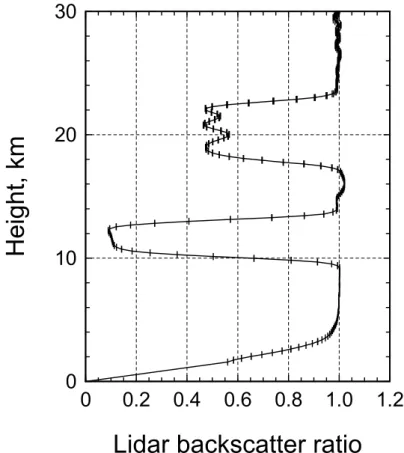
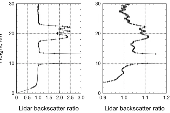
The lidar profile of 10/11 January 2003 is shown in Fig. 6. This shows two profoundly

5

depolarising layers – a cirrus layer below the tropopause (13 km) and a further layer between 18 and 22.5 km. This profile has again been analysed using the standard method (Fig. 7, using the Aberystwyth ozonesonde profile at 16:00 UT on 10 January) and shows a layer of aerosol with parallel backscatter ratio up to 1.12 and a perpendicu-lar backscatter ratio of up to 2.5 above 18 km, consistent with an aerosol depoperpendicu-larisation

10

of 18%.

These values are consistent with a Type 1a PSC (Toon et al., 1990), where a small number of relatively large particles give high depolarisation but little backscatter. This time, the minimum temperatures between 100 and 30 mb were <194 K, and maps of the 50 mb temperature field from ECMWF (obtained from the NADIR data base, NILU,

15

Norway) showed an extension of the polar vortex swinging east over the UK between 9 and 10 January; indeed, the ozonesonde launched on the 10 January resulted from an alert issued by the Match project (Rex et al., 2002). Observations on the following night (11/12 January) showed clear PSCs at the beginning of the night but not at the end, consistent with the retreat of the vortex northward during the 11 January. We believe

20

these to be the first lidar observations of PSCs reported from the UK.

5. Conclusions

We have used the dual polarisation method to infer lidar backscatter ratios in the lower stratosphere during background conditions. The method offers definite advantages over the “standard” method because uncertainty in the temperature profile can

(12)

ACPD

4, 6107–6126, 2004

Full Screen / Esc

Print Version

whelm the tiny amount of aerosol scattering, leading to an ill-characterised systematic error. With the system used here, several hours’ data must be collected to give enough signal at high altitude, but with a more powerful system this time could be reduced ten-fold. The system depolarisation was determined to be around 0.4±0.04%, a significant correction which must be measured each time an aerosol measurement is made.

5

We have shown that the background aerosol layer is quite variable – the few pro-files presented here show definite differences, even over a few days (other exam-ples, not shown here, support this assertion). On the whole, the peak lidar ratio at 20 km is around 1.03–1.06 and the integrated backscatter in background conditions 2–7×10−5sr−1.

10

We have also shown examples where the lidar encountered depolarising aerosol. Under such conditions the measurements cannot be used to derive a lidar ratio purely from the two lidar channels, emphasising that care is needed with this method. On the other hand, these observations are of geophysical interest, recording as they do the observation of Type 1A PSCs over the UK for the first time using a polarisation lidar.

15

Acknowledgements. We thank the NILU data base, Norway and the NERC BADC for provision of meteorological data for this study, and to the EC EARLINET project (EVRI-CT-1999-40003) for partial support.

References

Beyerle, G.: Detection of stratospheric sulphuric acid aerosols with polarisation lidar: theory, 20

simulations and observations, Applied Optics, 39, 4994–5000, 2000.

Cairo, F., Di Donfrancesco, G., Adriani, A., Pulvirenti, L., and Fierli, F.: Comparison of various linear depolarisation parameters measured by lidar, Applied Optics, 38, 4425–4432, 1999. J ¨ager, H.: European Research in the Stratosphere 1996–2000, Figure 2.27, edited by

Amana-tidis, G. T. and Harris, N. R. P., EUR19867, European Commission DGXII, Brussels, 2001. 25

J ¨ager, H. and Deshler, T.: Lidar backscatter to extinction, mass and area conversions for strato-spheric aerosols based on midlatitude balloonborne size distribution measurements, Geo-phys. Res. Lett., 29, art. no. 1929, 2002.

(13)

ACPD

4, 6107–6126, 2004

Full Screen / Esc

Print Version

J ¨ager, H. and Deshler, T.: Correction to “Lidar backscatter to extinction, mass and area con-versions for stratospheric aerosols based on midlatitude balloonborne size distribution mea-surements”, Geophys. Res. Lett., 30, art. no. 1382, 2003.

Rex, M., Salawitch, R. J., Harriset, N. R. P., et al.: Chemical depletion of Arctic ozone in winter 1999/2000, J. Geophys. Res., 107, art. no. 8276, 2002.

5

Siebert, J., Timmis, C., Vaughan, G., and Fricke, K. H.: A strange cloud in the Arctic summer stratosphere 1998 above Esrange (68◦N), Sweden, Ann. Geophys., 18, 505–509, 2000, SRef-ID:1432-0576/ag/2000-18-505.

Thomas, L. , Jenkins, D. B., Wareing, D. P., Vaughan, G., and Farrington, M.: Lidar observations of stratospheric aerosols associated with the El Chichon eruption, Ann. Geophys., 5A, 47– 10

56, 1987.

Toon, O. B., Browell, E. V., Kinne, S., and Jordan, J.: An analysis of lidar observations of polar stratospheric clouds, Geophys. Res. Lett. 17, 393–396, 1990.

Vaughan, G., Wareing, D. P., Pepler, S. J., Thomas, L., and Mitev, V.: Atmospheric temperature measurements by rotational Raman scattering, Applied Optics, 32, 2758–64, 1993.

15

Vaughan, G., Wareing, D. P., Jones, S. B., Thomas, L., and Larsen, N.: Lidar measurements of Mt. Pinatubo aerosols at Aberystwyth from August 1991 through March 1992, Geophys. Res. Lett., 21, 1315–1318, 1994.

(14)

ACPD

4, 6107–6126, 2004

Full Screen / Esc

Print Version

Max lidar ratio Integrated Backscatter, Comment (±0.01) 10−5sr−1(±2)

April 2601 1.04 6

May 0301 1.03 3

May 1201 1.03 3

May 22–2401 1.03 2 Combined 3 nights’ data December 1101 1.06 4

December 1201 1.06 5 October 0402 1.04 7 January 0603 1.06 7

January 07–0803 1.04 6 Depolarising aerosol

January 1003 1.12 10 PSCs

February 1804 1.06 7 February 2004 1.05 7 February 2204 1.04 7

(15)

ACPD

4, 6107–6126, 2004

Full Screen / Esc

Print Version Interactive Discussion © EGU 2004 Glass Beamsplitter PMT Perpendicular polariser Parallel polariser Interference filter Fig. 1. Schematic of lidar receiver.

(16)

ACPD

4, 6107–6126, 2004

Full Screen / Esc

0

10

20

30

0.90

0.95

1.00

1.05

1.10 Lidar backscatter ratio

Height, km

Fig. 2. Aerosol scattering 11/12 December 2001. Error bars denote the precision at each point

(17)

ACPD

4, 6107–6126, 2004

Full Screen / Esc

0

10

20

30

0.90

0.95

1.00

1.05

1.10 Feb18

Feb 22

Lidar backscatter ratio

Height, km

Fig. 3. Aerosol scattering 18 and 22 February 2004. Error bars denote the precision at each

(18)

ACPD

4, 6107–6126, 2004

Full Screen / Esc

0

10

20

30

0.90

0.95

1.00

1.05

1.10 Jan 08

Jan 07

Jan 06

Lidar backscatter ratio

Height, km

Fig. 4. Lidar ratio as derived from the two polarisations, 6–8 January 2003, showing aerosol

depolarisation in the lower stratosphere on 7 and 8 January. Each curve is derived from over 12 h continuous data. Error bars denote the precision at each point (1 standard deviation). Vertical resolution variable.

(19)

ACPD

4, 6107–6126, 2004

Full Screen / Esc

0

10

20

30

0.90

0.95

1.00

1.05

1.10 Lidar backscatter ratio

Height, km

Fig. 5. Ratio of lidar signals to synthetic density profiles, 8 January 2003. Solid line: ratio of ⊥

(20)

ACPD

4, 6107–6126, 2004

Full Screen / Esc

0

10

20

30

0

0.2

0.4

0.6

0.8

1.0

1.2 Lidar backscatter ratio

Height, km

Fig. 6. Lidar backscatter ratio measured 10–11 January 2003, showing two depolarising layers:

cirrus below 12 km and PSCs between 18.5 and 21.5 km. Error bars denote the precision at each point (1 standard deviation). Vertical resolution is 150 m, no smoothing.

(21)