CLABAUTAIR: a new algorithm for retrieving three-dimensional cloud structure from airborne microphysical measurements

(1)

HAL Id: hal-00304303

https://hal.archives-ouvertes.fr/hal-00304303

Submitted on 23 Dec 2004

HAL is a multi-disciplinary open access

archive for the deposit and dissemination of sci-entific research documents, whether they are pub-lished or not. The documents may come from teaching and research institutions in France or abroad, or from public or private research centers.

L’archive ouverte pluridisciplinaire HAL, est destinée au dépôt et à la diffusion de documents scientifiques de niveau recherche, publiés ou non, émanant des établissements d’enseignement et de recherche français ou étrangers, des laboratoires publics ou privés.

CLABAUTAIR: a new algorithm for retrieving

three-dimensional cloud structure from airborne

microphysical measurements

R. Scheirer, S. Schmidt

To cite this version:

R. Scheirer, S. Schmidt. CLABAUTAIR: a new algorithm for retrieving three-dimensional cloud structure from airborne microphysical measurements. Atmospheric Chemistry and Physics Discus-sions, European Geosciences Union, 2004, 4 (6), pp.8609-8625. �hal-00304303�

(2)

ACPD

4, 8609–8625, 2004 Retrieving cloud structure from airborne measurements R. Scheirer and S. Schmidt Title Page Abstract Introduction Conclusions References Tables Figures J I J I Back Close Full Screen / Esc

Print Version Interactive Discussion

Atmos. Chem. Phys. Discuss., 4, 8609–8625, 2004 www.atmos-chem-phys.org/acpd/4/8609/

SRef-ID: 1680-7375/acpd/2004-4-8609 European Geosciences Union

Atmospheric Chemistry and Physics Discussions

CLABAUTAIR: a new algorithm for

retrieving three-dimensional cloud

structure from airborne microphysical

measurements

R. Scheirer1and S. Schmidt2

1_{Institut f ¨ur Physik der Atmosph ¨are, DLR, Oberpfaffenhofen, Germany} 2

Leibniz-Institute for Tropospheric Research, Leipzig, Germany

Received: 20 October 2004 – Accepted: 7 December 2004 – Published: 23 December 2004 Correspondence to: R. Scheirer (ronald.scheirer@dlr.de)

(3)

ACPD

Abstract

A new algorithm is presented to retrieve the three-dimensional structure of clouds from airborne measurements of microphysical parameters. Data from individual flight legs are scanned for characteristic patterns, and the autocorrelation functions for several directions are used to extrapolate the observations along the flight path to a full three-5

dimensional distribution of the cloud field. Thereby, the mean measured profiles of microphysical parameters are imposed to the cloud field by mapping the measured probability density functions onto the model layers. The algorithm was tested by simu-lating flight legs through synthetic clouds (by means of Large Eddy Simulations (LES)) and applied to a stratocumulus cloud case measured during the first field experiment 10

of the EC project INSPECTRO (INfluence of clouds on the SPECtral actinic flux in the lower TROposphere) in East Anglia, UK. The number and position of the flight tracks determine the quality of the retrieved cloud field. If they provide a representative sam-ple of the entire field, the derived pattern closely resembles the statistical properties of the real cloud field.

15

1. Introduction

A challenge in three-dimensional (3-D) radiative transfer is the generation of realis-tic clouds as input for sophisrealis-ticated radiative transfer models (e.g. Borde and Isaka, 1996; Petty, 2002). Currently, it is not possible to derive the required distribution of liquid water content and droplet sizes from observations of a single instrument. Pas-20

sive satellite remote sensing instruments may provide a detailed horizontal distribution but fail to give reliable information about vertical profiles (e.g. Crewell et al., 1999). In-situ observations, on the other hand, may give data for any location but are usually restricted to only a few point measurements, e.g. along an aircraft flight track. Physical cloud-models (e.g. LES) can provide the full 3-D information of all needed microphys-25

(4)

ACPD

(Stevens and Lenschow, 2001).

Clouds vary significantly in the three spatial dimensions and in time. Common air-borne instruments sample volumes in the magnitude of a few liters during a single leg while cumulus clouds, for example, often cover a volume of around 109m3. The major part of the clouds are thus not considered for its characterization which is a significant 5

limitation because of the cloud’s large variability (Evans et al., 2003). Therefore, aircraft measurements alone seem to be generally not sufficient to characterize the properties of inhomogeneous cloud layers.

On the other hand the spatial distribution of cloud droplets exhibit rather a patchy structure than following Poisson statistics (i.e. droplet concentrations in two adjacent 10

volumes won’t show an independent behavior), so that there should be a spatial cor-relation of droplet concentrations (Kostinski and Jameson, 2000). This structure is organized by entrainment and turbulence at several length scales. For micro-scale tur-bulence this is shown by Shaw et al. (1998). The turbulent spectrum is determined by the state of the atmosphere. For homogeneous conditions within a limited area and 15

time period, a similar behavior of the corresponding cloud field is expected. Thus, in some cases such as for stratiform overcast or broken cloud fields, aircraft line measure-ments along a limited number of flight legs are representative for the whole layer under stable conditions. For example, Los and Duynkerke (2000) and R ¨ais ¨anen et al. (2003) generated two-dimensional cloud fields from in-cloud aircraft measurements. How-20

ever, they required some assumptions about cloud top and base structure, and about the profile of microphysical parameters.

This study introduces a new algorithm which generates 3-D cloud fields using aircraft measurements of liquid water content and effective radius without additional assump-tions. In Sect.2, the extrapolation of the 3-D structure from one-dimensional aircraft 25

measurements, and thus the filling of the gaps is described. Subsequently, the al-gorithm is applied to a synthetic cloud field (Sect. 3) and to a measured cloud case (Sect.4), and a preliminary discussion of its applicability is given.

(5)

ACPD

2. Algorithm

An automated algorithm (CLoud liquid wAter content and effective radius retrieval By an AUTomated use of AIRcraft measurements (CLABAUTAIR)) has been developed with the intention to generate a 3-D cloud field which reproduces the statistical prop-erties of the microphysical aircraft measurements without introducing any additional 5

assumptions about the cloud structure. The measurements of liquid water content (LW C) and effective radius (Reff) are scanned, and the probability density functions “PDFs” as well as the autocorrelation functions are determined for every layer, defined by the user. The patterns which are found in the autocorrelation functions are then used to extrapolate the aircraft data to a complete 3-D field.

10

This method is illustrated in Fig.1a–d. Starting with measurements in a single hor-izontal layer the main directions sampled by the aircraft are identified. This means, the data-points are sampled by relative angular (e.g. directions from one point to each other point) bins layer by layer, to spot long straight lines of measurements (Fig.1a). This is necessary to avoid aliasing due to the connection of different flight legs and 15

thus to correlate only data collected within a time interval during which the cloud can be considered constant. Next, the autocorrelation functions along these directions are calculated (Fig.1b).

Then the measured LW C and Reff are replaced by their anomalies (i.e. deviations from the layers mean). To extrapolate the observations, individual empty boxes are 20

randomly selected within the 3-D space. The requested parameters ξ (anomaly of

LW C or Reff) for each of these boxes are calculated by a weighted average over the I filled boxes along the J main directions (Fig.1c). The weighting is performed by the autocorrelation coefficient r valid for the distance δ=|x − x_{i ,j}| between the center of the current (already filled) box at (x_{i ,j}) and the i th box under calculation for the j th direction 25

(6)

ACPD

at (x) (marked with a question mark in Fig.1c):

ξ(x)= J P j=1 I(j ) P i=1 r_j(|x − x_{i ,j}|)ξ(x_{i ,j}) J P j=1 I(j ) P i=1 |r_j(|x − x_{i ,j}|)| (1)

If the weighting sum

J X j=1 I(j ) X i=1 |r_j(|x − x_{i ,j}|)| (2)

fails to reach a certain threshold, calculation of ξ(x) will be postponed. Initially1 this 5

threshold is set to 3 to take into account only calculations with a minimum attendance of contributing boxes. Due to the use of anomalies instead of absolute values this approach is also meaningful in case of negative autocorrelation coefficients. Adjacent boxes from the next layer above and below the chosen one (if already calculated) are taken into account with a fixed weight2of 0.95. This step is repeated until all boxes are 10

filled. Finally, the “PDF” of the measurements (including the cloud-free parts to permit cloud fractions smaller than 1) are mapped onto the thus derived spatial distributions. This is done for all cloudy layers separately. Figure1d shows the final cloud field.

The possible spatial resolution depends on the number, the direction, and the length of the flight legs, the sampling rate, and on the autocorrelation function. For the cases 15

used in this study, horizontal resolutions between 50 m and 250 m and vertical resolu-tions between 50 m and 100 m were used.

1

if this threshold results in accepting less than 1% of the calculations it will be reduced temporarily.

2

Actually this weight depends on the vertical resolution but for magnitudes used in this study, the stated weight is reasonable.

(7)

ACPD

3. Test of the method

The algorithm was tested with a synthetic cloud field. A large eddy simulation (LE S) of a stratocumulus field provided by the Intercomparison of 3-D Radiation Codes (I3RC, at

http://i3rc.gsfc.nasa.gov) was chosen for this test. The LE S cloud field has a horizontal resolution of 55 m and a vertical resolution of 25 m. With 64 times 64 boxes the domain 5

size is 3.5×3.5 km2. The clouds are located between 400 m and 800 m altitude. Within this cloud field samples were taken by virtual flights. The flight starts at the center of the area at the ground with a random direction and an ascent angel of 10◦. A new direction is selected by random if the border is reached. If cloud top is exceeded, the descend starts in the same manner but at a flatter angle (0.5◦). Samples are taken 10

every 10 m with a random error of ±5% added to the data. Typically about 2% of the total model boxes are described by virtual measurements so that about 98% had to be calculated by our algorithm.

For the retrieved cloud field, the horizontal resolution was set to 43 m and the vertical to 39 m to avoid the unrealistic case of model boxes that fit perfectly to the source 15

cloud. Three examples of different flight patterns and the resulting retrievals are given in Fig. 2. We found that the gain in information by following the same flight-track at different altitudes is marginal (left column) because of the large vertical correlation of microphysical properties. Therefore we recommend random-like flight patterns (middle and right column) to get more independent information and to sample a larger area. 20

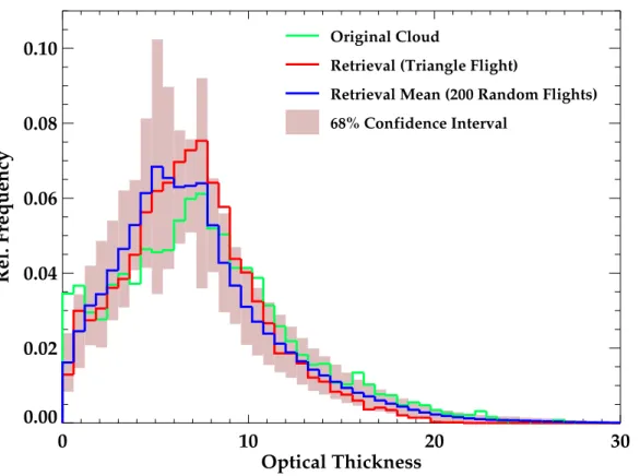
Figure3shows the frequency of optical thicknesses for the original cloud field as well as for the retrieval-mean of 200 random flights. The original cloud-fraction is 0.926 while the retrieval-mean gives 0.959 with a standard deviation of 0.018. For the cloud volume the retrieval provides a mean of 1.860 km3and a standard deviation of 0.123 km3while the original volume is 1.874 km3. So we found CLABAUTAIR to reproduce the cloud 25

(8)

ACPD

4. Application to field measurements

4.1. Aircraft data

The first application of the algorithm to in-situ microphysical data was performed for a cloud situation which was measured during the first field experiment of the EC project INSPECTRO (INfluence of clouds on the SPECtral actinic flux in the lower TROpo-5

sphere) on 14 September 2002, on the coast of East Anglia, United Kingdom. On this day, a stable stratus layer which was moving into land at a speed of about 10 m/s was observed between 500 and 1100 m altitude. The microphysical measurements used for this study were performed with a two-propeller research aircraft, a Partenavia P68B, which was equipped with meteorological, microphysical, and radiation instrumentation. 10

The microphysical cloud properties were measured with a Fast Forward Scattering Spectrometer Probe (Fast-FSSP, Brenguier et al., 1998) and a Particle Volume Monitor (PVM-100, Gerber et al., 1994). The Fast-FSSP measures the cloud drop size distri-bution by detecting the forward scattering signal of each individual droplet passing a laser beam. From the drop size distribution, bulk parameters such as the LW C, the 15

drop concentration, and Reff can be derived (Schmidt, 2004). In contrast, the PVM-100A measures the LW C directly by detecting the scattering signal of an ensemble of droplets. For this study, the LW C measurements by the PVM-100A were used be-cause of the high accuracy and temporal resolution of the data. The effective droplet radius Reff was derived from the FSSP measurements because of its higher accuracy 20

for size distributions.

In order to examine the three-dimensional cloud structure, several ascents and de-scents through the cloud layer were flown by the aircraft. In addition, one triangular flight pattern within the layer was performed. Figure 4 shows the two-dimensional “PDFs” of the LW C and Reff for three different altitudes. They were determined by 25

combining the measurements of the PVM-100A and the Fast-FSSP, and binning them into several height layers. The color scale in the plots corresponds to the probability of a particular LW C and Reff at the respective level. These two-dimensional “PDFs” reflect

(9)

ACPD

the microphysical properties accumulated throughout the cloud layer. The layer cloud fraction as a macrophysical property is also deduced from the microphysical measure-ments. The horizontal structure is contained in the autocorrelation functions which are calculated for the three legs of the triangle.

4.2. Retrieved cloud fields 5

For the INSPECTRO cloud case which is described in Sect.4.1, the output of the algo-rithm was quantitatively compared with the measurements by analyzing the measured and retrieved profiles of the LW C and the power spectra along horizontal lines.

In Fig.5, measured and reconstructed profiles of the LW C are displayed. The circles show the PVM-100A measurements. At 800 m, the horizontal flight pattern was per-10

formed. The range of LW C values measured at this altitude reflects the high variability which prevails even in a stratus layer. The solid blue line shows the mean reconstructed

LW C profile. The error bars indicate the standard deviation which was found

through-out the grid. It reproduces well the range of LW C values which were measured during the horizontal leg. The dashed and dash-dotted blue lines correspond to the maximum 15

and minimum LW C values, respectively, which are generated at the levels. The cloud top and base heights vary approximately within 200 m.

The horizontal structure of the measured and reconstructed cloud is compared in Fig.6by means of power spectra P (k) where k denotes the wavenumber. The dotted line with open circles shows the power spectrum which was calculated from PVM-100A 20

measurements along one of the legs of the triangular pattern within the cloud layer (about 20 km length). The measurements are in agreement with the k−5/3 scaling law (thin solid line) which is typically found for real clouds (Davis et al., 1996). The power spectra from the reproduced cloud were obtained by calculating power spectra over horizontal lines throughout the grid and by subsequent averaging. The direction of the 25

lines was chosen along and across the flight leg whose power spectrum is displayed. The red line shows the averaged power spectrum of lines parallel to the leg direction.

(10)

ACPD

In general the k−5/3 scaling is well reproduced. However, the variability is slightly over-estimated by the generator for large wavenumbers. The blue line shows the averaged power spectrum from lines across the leg direction. In this case, the variability shows a better agreement with the measurements. The power spectra for the PVM-100A data measured along other legs of the in-cloud pattern are similar to the power spectrum 5

which is displayed in Fig.6. Thus, the differences between power spectra along differ-ent directions of the reproduced cloud field cannot be explained by the measuremdiffer-ents. However, the power spectra of the reproduced cloud field agree with the observations within the range of measurement uncertainty.

5. Conclusions

10

A new algorithm for the retrieval of 3-D cloud fields based on aircraft measurements has been developed.

Testing our algorithm with a complete LES cloud field, we found a promising agree-ment between the original and retrieved cloud features. The retrieval mean cloud-fraction provides an error of about 3.6% and the retrieval mean cloud-volume an error 15

of about 0.8%. For the sampling of cloud fields we recommend to follow random-like instead of flight patterns that imply similar paths at different altitudes.

From an application to real measurements we learned that within the measurement uncertainty, the characteristics of the simulated clouds agree with the observed coun-terparts.

20

It must be stated that the presented algorithm is limited to a moderate wind-speed and stable conditions, i.e. no significant change in the cloud pattern should occur during the measurements (no rapid convective growth). Rather than reproducing the original cloud situation, CLABAUTAIR supplies a cloud field whose statistical properties match the aircraft measurements. This could also be valid for the spiky behavior (the intermit-25

(11)

ACPD

if the database is really representative. Nevertheless, additional work will be done on validation and improvement of the presented algorithm.

Acknowledgements. This work was funded by the European project INSPECTRO (Influence

of clouds on the spectral actinic flux in the lower troposphere), contract EVK2-2001-00135. Enviscope GmbH, Frankfurt, Germany, operated the aircraft during the experiment: Thanks to 5

R. Maser, D. Schell, and H. Franke, and to the pilot B. Schumacher. L. Hinkelman, Langley Research Center, Hampton, USA provided us with LES cloud fields used for preliminary tests.

References

Borde, R. and Isaka, H.: Radiative transfer in multifractal clouds, J. Geophys. Res., 101(D23), 29 461–29 478, 1996.

10

Brenguier, J. L., Bourrianne, T., Coelho, A., Isbert, J., Peytavi, R., Trevarin, D., and Weschler, P.: Improvements of droplet size distribution measurements with the Fast-FSSP (Forward Scattering Spectrometer Probe). J. Atmos. Oceanic Technol., 15, 1077–1090, 1998.

Crewell, S., Hasse, G., L ¨ohnert, U., Mebold, H., and Simmer, C.: A Ground Based Multi-Sensor System for the Remote Sensing of Clouds, Phys. Chem. Earth (B), 24, 207–211, 1999. 15

Davis, A., Marshak, A., Wiscombe, W., and Cahalan, R.: Multifractal characterizations of non-stationarity and intermittency in geophysical fields: Observed, retrieved, or simulated, J. Geophys. Res., 99(D4), 8055–8072, 1994.

Davis, A., Marshak, A., Wiscombe, W., and Cahalan, R.: Scale Invariance of Liquid Water Distributions in Marine Stratocumulus, Part I: Spectral Properties and Stationarity Issues, J. 20

Atmos. Sci., 53, 1538–1558, 1996.

Evans, K. F., Lawson, R. P., Zmarzly, P., O’Connor, D., and Wiscombe, W. J.: In situ cloud sens-ing with multiple scattersens-ing lidar: Simulations and demonstration, J. Atmos. Ocean Tech., 20, 1505–1522, 2003.

Gerber, H., Ahrends, B. G., and Ackerman, A. S.: New microphysics sensor for aircraft use, 25

Atmos. Res., 31, 235–252, 1994.

Kostinski, A. B. and Jameson, A. R.: On the Spatial Distribution of Cloud Particles, J. Atmos. Sci., 57, 901–915, 2000.

(12)

stra-ACPD

tocumulus: Observations and model simulations, Quart. J. R. Meteorol. Soc., 126, 3287– 3307, 2000.

Petty, G. W.: Area-Average Solar Radiative Transfer in Three-Dimensionally Inhomogeneous Clouds: The Independently Scattering Cloudlet Model, J. Atmos. Sci., 59, 2910–2929, 2002. R ¨ais ¨anen, P., Isaac, G. A., Barker, H. W., and Gultepe, I.: Solar radiative transfer for stratiform 5

clouds with horizontal variations in liquid-water path and droplet effective radius, Quart. J. R. Meteorol. Soc., 129, 2135–2149, 2003.

Schmidt, S.: Influence of Cloud Inhomogeneities on Solar Spectral Radiation, PhD thesis, 105, Univ. Leipzig, Germany, Leipzig, 9 July 2004.

Shaw, R. A., Reade, W. C., Collins, L. R., and Verlinde, J.: Preferential concentration of cloud 10

droplets by turbulence: Effects on the early evolution of cumulus cloud droplet spectra, J. Atmos. Sci., 55, 1965–1976, 1998.

Stevens, B. and Lenschow, D. H.: Observations, experiments and large eddy simulation, Bull. Amer. Meteor. Soc., 82, 283–294, 2001.

(13)

ACPD

Print Version Interactive Discussion X Y Y X Y X Y X d) b) c) a) ?

Fig. 1. The four main steps of CLABAUTAIR. This figure illustrates an approach to retrieve 3-D

(14)

ACPD

Fig. 2. Three examples of different flight patterns within a LES cloud field (upper row). Red

arrows mark ascending and blue arrows descending legs. Considered are only flight legs meeting the cloudy altitudes (400 m–800 m). The retrieved cloud structures are given in the lower row.

(15)

ACPD

Print Version Interactive Discussion 0 10 20 30 Optical Thickness 0.00 0.02 0.04 0.06 0.08 0.10 Rel. Frequency Original Cloud

Retrieval (Triangle Flight)

Retrieval Mean (200 Random Flights) 68% Confidence Interval

Fig. 3. Frequency of optical thicknesses for the original cloud field (green), the retrieval from

triangular flight (red), and the mean of 200 retrievals (blue). The shaded area marks the 68% confidence interval.

(16)

ACPD

4 5 6 7 8 9

0.3

0.4

0.5

0.6

0.7

0.8 0.9 700 m

R

_eff

[µm]

LWC

[g m

-3

]

0.01 0.02 0.03 0.04 0.05 0.06 0.07 0.08 0.09 0.1

4 5 6 7 8 9

0.3

0.4

0.5

0.6

0.7

0.8

0.9 R

_eff

[µm]

800 m

4 5 6 7 8 9

0.3

0.4

0.5

0.6

0.7

0.8

0.9 _{900 m}

R

_eff

[µm]

Fig. 4. Two-dimensional “PDF” of the measured liquid water content and the effective drop

(17)

ACPD

400 500 600 700 800 900 1000 1100 1200

0.0

0.2

0.4

0.6

0.8

1.0 measured (PVM)

reconstructed

mean

minimum

maximum

LWC

[g m

-3

]

Altitude [m]

(18)

ACPD

0.1

1 1E-5

1E-4

1E-3

0.01

0.1

1 Power Spectra

measured along track

reconstructed

along track

across track

n

-5/3

P

n

[(g/m

3

/(1/km))

2