Has spring snowpack declined in the Washington Cascades?

(1)

HAL Id: hal-00298855

https://hal.archives-ouvertes.fr/hal-00298855

Submitted on 5 Jul 2007

HAL is a multi-disciplinary open access

archive for the deposit and dissemination of sci-entific research documents, whether they are pub-lished or not. The documents may come from teaching and research institutions in France or abroad, or from public or private research centers.

L’archive ouverte pluridisciplinaire HAL, est destinée au dépôt et à la diffusion de documents scientifiques de niveau recherche, publiés ou non, émanant des établissements d’enseignement et de recherche français ou étrangers, des laboratoires publics ou privés.

Has spring snowpack declined in the Washington

Cascades?

P. Mote, A. Hamlet, E. Salathé

To cite this version:

P. Mote, A. Hamlet, E. Salathé. Has spring snowpack declined in the Washington Cascades?. Hydrol-ogy and Earth System Sciences Discussions, European Geosciences Union, 2007, 4 (4), pp.2073-2110. �hal-00298855�

(2)

HESSD

4, 2073–2110, 2007

Has spring snowpack declined in the Washington Cascades? P. Mote et al. Title Page Abstract Introduction Conclusions References Tables Figures ◭ ◮ ◭ ◮ Back Close Full Screen / Esc

Printer-friendly Version Interactive Discussion Hydrol. Earth Syst. Sci. Discuss., 4, 2073–2110, 2007

www.hydrol-earth-syst-sci-discuss.net/4/2073/2007/ © Author(s) 2007. This work is licensed

under a Creative Commons License.

Hydrology and Earth System Sciences Discussions

Papers published in Hydrology and Earth System Sciences Discussions are under open-access review for the journal Hydrology and Earth System Sciences

Has spring snowpack declined in the

Washington Cascades?

P. Mote1, A. Hamlet1,2, and E. Salath ´e1

1

Climate Impacts Group, University of Washington, Seattle, USA

2

Department of Civil and Environmental Engineering, University of Washington, Seattle, USA Received: 26 June 2007 – Accepted: 26 June 2007 – Published: 5 July 2007

Correspondence to: P. Mote (philip@atmos.washington.edu)

(3)

HESSD

4, 2073–2110, 2007

Printer-friendly Version Interactive Discussion

Abstract

Our best estimates of 1 April snow water equivalent (SWE) in the Cascade Mountains of Washington State indicate a substantial (roughly 15–35%) decline from mid-century to 2006, with larger declines at low elevations and smaller declines or increases at high elevations. This range of values includes estimates from observations and hydrologic

5

modeling, reflects a range of starting points between about 1930 and 1970 and also reflects uncertainties about sampling. The most important sampling issue springs from the fact that half the 1 April SWE in the Cascades is found below about 1000 m, where sampling was poor before 1945. Separating the influences of temperature and precip-itation on 1 April SWE in several ways, it is clear that long-term trends are dominated

10

by trends in temperature, whereas variability in precipitation adds “noise” to the time series. Consideration of spatial and temporal patterns of change rules out natural vari-ations like the Pacific Decadal Oscillation as the sole cause of the decline. Regional warming has clearly played a role, but it is not yet possible to quantify how much of that regional warming is related to greenhouse gas emissions.

15

1 Introduction

Phase changes of water from ice to liquid are among the most visible results of a warming climate, and include declines in summer Arctic sea ice, the Greenland ice sheet, and most of the world’s glaciers (Lemke et al., 2007). These components of the cryosphere have slow response times and take decades to centuries to come into

20

equilibrium with a change in climate. By contrast, seasonal snow cover disappears every year and therefore each year’s snow cover is the product of a single year’s climate conditions. This makes changes happen more rapidly but also substantially decreases the signal-to-noise ratio.

Northern hemisphere spring snow cover has declined about 8% over the period of

25

record 1922–2005 (Lemke et al., 2007) and the declines have predominantly occurred 2074

(4)

HESSD

4, 2073–2110, 2007

Printer-friendly Version Interactive Discussion between the 0◦ _{and 5}◦_{C isotherms, underscoring the feedbacks between snow and}

temperature near the freezing point. That is, small amounts of warming can provide the impetus to melt snow, which increases absorption of solar radiation by the under-lying surface and provides additional warming. This feedback is particularly strong in spring in lower latitudes when solar radiation is rather strong; in winter solar radiation

5

is considerably weaker, which helps explain why large-scale declines in December and January are small to nonexistent.

For the mountainous regions of the western U.S., summers are usually dry and snowmelt provides approximately 70% of annual streamflow. Observations of moun-tain snowpack in the spring provide important predictions of summer streamflow for

10

agriculture, hydropower, and flood control, among other needs. These mountain snow observations also provide a unique climate record of changes in the mountains, and demonstrate long-term declines at approximately 75% of sites since 1950 (Mote et al., 2005) or 1960 (Mote, 2006). The enormous importance of snowmelt for western water resources, and the sensitivity of snow accumulation and melt to air temperature,

pro-15

vide strong motivations for better understanding the role that warming has played in regional changes in snowpack.

Bales et al. (2006) estimated the fraction of annual precipitation falling between 0◦C and –3◦_{C, what one might call warm snow. The Cascade and Olympic Mountains}

of Washington and Oregon stand out as having the highest fraction of warm snow

20

in the continental U.S. In this paper we examine changes in areally averaged 1 April SWE, with three purposes in mind: First, to provide greater spatial specificity to the results of Mote et al. (2005); second, to demonstrate the challenges in quantifying such change; and third, to determine whether a human influence on snowpack can be detected. This third point exploits the facts that a human influence on climate can

25

be detected as a warming, at least on the scale of the western U.S. (Stott, 2003), that the best estimates of anthropogenic change in precipitation for the Northwest are for no measurable change (Salathe et al., 2007); and that the pattern of response to warming is to lose more snow at low elevations than at high elevations (Mote et al.,

(5)

HESSD

4, 2073–2110, 2007

Printer-friendly Version Interactive Discussion 2005; Regonda et al., 2005).

2 Data and methods

Snow surveys have been conducted at over a thousand carefully surveyed and marked locations, or “snow courses”, in western North America for decades. When new snow courses were established, surveyors had several goals in siting them, for example to

5

minimize the effects of blowing snow by siting the snow courses in natural clearings on relatively level terrain, generally in bowls or benches. Since the purpose was water supply forecasting, the measurements of SWE were most prevalent initially near the date of peak SWE, 1 April. Over time the sites were typically visited more frequently, monthly from 1 January to 1 June. Automated sites began to be used in the 1980s

10

and in some cases replaced snow courses. For Washington’s Cascades (west of 120◦

longitude) and Olympics, 49 long term records are available (Fig. 1, Table 1). Spatial coverage is uneven, and was especially uneven before 1938 when all snow courses (and aerial markers) were at high elevation in the North Cascades.

The data are provided by the Natural Resources Conservation Service (NRCS) of

15

the US Department of Agriculture (http://www.wcc.nrcs.usda.gov/snow/snowhist.html). Climate data came from the Western Regional Climate Center (http://www.wrcc.dri.

edu/cgi-bin/divplot1 form.pl?4504). The North Pacific Index (NPI) was obtained from

http://www.cgd.ucar.edu/∼_{jhurrell/np.html}_{. Detailed consideration of individual time}

se-ries is beyond the scope of this paper, but users can plot maps of linear trends and also

20

time series at individual sites athttp://www.climate.washington.edu/trendanalysis/. The smoothing performed in some of the figures uses the locally weighted regression (“loess”) scheme (Cleveland, 1993) with partial reflection. Loess computes each value for the smoothed time series by performing a least-squares linear fit on weighted adja-cent data, where the analyst determines a suitable window to define adjaadja-cent and the

25

weighting favors closer points. The smoothing parameter α is chosen so that the resid-uals have very little low-frequency variability; in this case α=0.6. To handle variations

(6)

HESSD

4, 2073–2110, 2007

Printer-friendly Version Interactive Discussion near the endpoints, a linear combination of two loess-smoothed versions is used: first,

the original time series, for which the end points are somewhat weakly constrained, and second, the middle third of a time series formed by reflecting the original time se-ries (x1,...xj) about its endpoints (xj...x1,x1,... xj, xj...x1) with the result that the first

derivative of the curve must be zero at the endpoints. This “partial reflection” approach

5

seems to produce the best results at the endpoints.

For calculating statistical significance, a two-sided t-test (p<0.05) is used, and de-grees of freedom are first estimated by checking for autocorrelation. In the time series shown here, the lag-1 autocorrelation is negative, so the number of degrees of freedom is simply the number of data points.

10

3 Simulation with the VIC hydrology model

Physically based hydrologic models can be used to achieve some of the goals of this study, by providing spatially uniform fields of estimation and also evaluating the climatic factors behind the variability and trends in snowpack. In this study (as in Mote et al., 2005, and Hamlet et al., 2005) we use the Variable Infiltration Capacity (VIC) hydrologic

15

model (Liang et al., 1994; Cherkauer and Lettenmaier, 2003) implemented over the western U.S. at 1/8th degree spatial resolution. As inputs to the VIC model, we used a gridded dataset of daily precipitation and maximum and minimum temperature (Hamlet and Lettenmaier 2005), at the same 1/8th degree resolution, from 1915 to 2003. Spatial interpolation of daily data from the Cooperative weather (Coop) network, with

terrain-20

dependent algorithms, provide the spatial coverage. The temporal characteristics of the dataset are nudged toward the monthly values from the climate-quality dataset from the Historical Climatology Network (HCN) (Karl et al., 1990). The methods used to produce the driving data, and evaluation of the resulting hydrologic simulations using observed streamflow records, are reported in more detail by Hamlet and Lettenmaier

25

(2005). The VIC simulation was conducted at a daily time step for the water balance and at a time step of one hour for the snow model. Additional details on the hydrologic

(7)

HESSD

4, 2073–2110, 2007

Printer-friendly Version Interactive Discussion model and its implementation are reported by Hamlet et al. (2005).

Using VIC simulations of snow over the Western U.S., Mote et al. (2005) corrobo-rated observed trends in snowpack derived from snow course observations from 1950– 1997. The model was shown to do a remarkably good job of reproducing topographic gradients in snowpack trends over the West as a whole and particularly in the

Cas-5

cades in the Pacific Northwest. Based on this evaluation of the model, the simulations were extended to 1915–2003 and long term trends in snowpack for several different periods from 1915–2003 were examined (Hamlet et al., 2005). That study also exam-ined, in detail, the relative roles of temperature and precipitation trends on snowpack trends in each period.

10

We now examine the performance of the VIC model at the snow courses in Wash-ington over the period 1950–1997. Note first that there are several reasons why the SWE simulated by VIC and the SWE measured at a snow course might differ: terrain, temporal offsets, interpolation of driving data, spurious trends in driving data, and land-cover change at the snow course. These are discussed more by Mote et al. (2005).

15

First, while a VIC grid cell includes 15 snow “bands” with different elevation and land cover over a roughly 10×12 km area, a snow course reports the snowpack at a spe-cific site in terrain that may or may not be representative of a larger area, though the locations for snow courses are chosen with the goal of representing SWE over a signif-icant portion of a watershed. Second, the actual date of a snow course measurement

20

can be several days before 1 April, so a storm or melt event between the observation date and the 1 April VIC date. Third, VIC uses weather data from stations that may be 50 km or more from the grid cell and may not represent local hydroclimatic conditions despite the efforts of the terrain-dependent algorithm to do so. Fourth, the driving data (especially precipitation) might contain spurious trends owing, for example, to growth

25

of trees over a rain gauge; efforts are made in constructing the HCN dataset to find and correct such sources of error, but some undoubtedly remain. Finally, changes in land cover (e.g., incursion of forest into a previously open area) at the site of the snow course may also introduce trends that are not shared over the 10×12 km area of a VIC

(8)

HESSD

4, 2073–2110, 2007

Printer-friendly Version Interactive Discussion grid cell. For all these reasons, and probably more, we would not expect a close match

between the mean VIC grid cell value and the mean snow course value nor between the trends.

Despite these potential sources of differences between VIC SWE and observed SWE, Table 2 and Fig. 2 show a strong correspondence at about three-quarters of

5

the snow courses examined. Correlations are fairly high, with a median of 0.8, rms differences are typically a small fraction of the mean, with a median of 18 cm, and the median absolute difference in the trends is 16%. For about a quarter of the sites, trends disagree by more than 26% as with Deer Park and Dock Butte aerial marker (AM) shown here. From this analysis it is impossible to deduce the reasons for the

dis-10

crepancies between VIC and observations at some sites. The strong correspondence at the majority of sites, though, combined with the previously demonstrated success of VIC at simulating streamflow in this region, provides a strong basis for using VIC to produce spatially averaged estimates of total 1 April SWE.

Figure 3a shows the results of spatially averaging the VIC 1 April SWE over the

Cas-15

cades domain for the 1916–2003 period of record. Note that a number of low-elevation grid cells with no snow on 1 April are included in the domain for averaging, which pro-duces a much lower average SWE than the observed time series we construct below. The interannual variability of the time series shown in Fig. 3a is substantial, with a co-efficient of variation of 0.35. Highest 1 April SWE occurred in 1956, followed by 1997,

20

1950, and 1999; very low values occurred in 1941, 1977, and 1992. The smooth curve shows the interdecadal variability, with relatively snowy periods centered around 1950, 1970, and 1999, and relatively snow-poor periods centered around 1992 and 1926. A linear fit to the entire period of record gives a decline of 16%. We will explore below the choice of starting date for reporting period-of-record trend.

25

In order to elucidate the climatic factors behind these changes, we examine also a simulation discussed by Hamlet et al. (2005, which see for details) in which the interannual variability in precipitation is removed from the driving dataset. This way, interannual variability in SWE is produced primarily from variations in temperature. The

(9)

HESSD

4, 2073–2110, 2007

Printer-friendly Version Interactive Discussion result (Fig. 3b) has substantially less interannual variability, and slightly smaller trend

(13%). Trends since 1950 were larger, but again were dominated by temperature not by precipitation.

4 Challenges in quantifying “the snowpack” of a mountain range

Using observations to estimate the total snow in a mountain range at a given time is

5

difficult for several reasons, some of which were discussed above in connection with the VIC simulation. Precipitation varies strongly with altitude, aspect, and slope, and local winds interacting with terrain and vegetation cover can redistribute falling snow leading to drifts, bare spots, and other heterogeneous features. Over the course of the winter, melt events may remove snowpack as runoff or infiltration into the soil, and

10

may also change or “ripen” the snowpack. Point measurements of snow depth or snow water equivalent (SWE) are subject to all of these factors and more.

Sampling is another important consideration. Estimating the total SWE for a moun-tain range depends very much on the choices one makes about which snow courses to include. Horizontal coverage is one factor – note the patchiness of coverage in

15

Fig. 1, with some river basins well-sampled and others unsampled. Ideally, an ob-servationally derived estimate would balance spatial coverage with temporal longevity. However, another crucial factor, even more than horizontal coverage, is vertical cov-erage. As Fig. 4a shows, the number of long-term snow courses (those in existence by 1960 and still providing data in 2006) changed rapidly during the 1940s, so that

20

the choice of a cutoff year (say 1945 or 1950) influences how many snow courses are available for analysis and their mean elevation. In particular, the early courses had a much higher mean elevation before about 1945, when the mean elevation stabilized at about 1300 m. This fact is crucially important in selecting snow courses because (a) according to our estimates from observations (below) and from VIC, roughly half

25

the snowpack in the Cascades on 1 April lies at elevations below about 1000 m, so it is important to adequately sample that half of the snowpack; and (b) low-elevation

(10)

HESSD

4, 2073–2110, 2007

Printer-friendly Version Interactive Discussion snowpack is much more sensitive to temperature than high-elevation snowpack (Mote,

2003, Mote et al., 2005, Hamlet et al. 2005), hence any response to regional warming is most likely to be detectable at lower elevations. Consequently, requiring that snow courses be active before about 1945 leads to a considerable sampling bias. As we will show below, there are ways of judiciously addressing this sampling bias to estimate

5

variability before 1945.

Another consequence of the choice of starting date concerns the grand mean SWE for the available snow courses. High elevation snow courses also have higher mean SWE. Fig. 4b shows the mean SWE and elevation for each of the snow courses, and shows how the lower elevations were poorly sampled before 1940 and much better

10

sampled by 1945. The grand mean was lower in 1940 than in 1945.

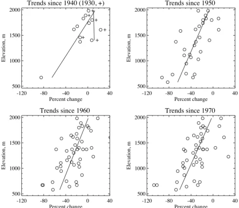
As shown by Mote et al. (2005) and Mote (2006), the clearest signature of warming-induced changes in snowpack is that trends become more positive with increasing elevation. Figure 5 shows how consistently the trends depend on elevation, regardless (to first order) of starting year, with lines drawn to indicate how the trends depend

15

quantitatively on elevation. The slopes of the lines are 59±28%/1000 m for 1940-present, 40±13%/1000 m for 1950-1940-present, 37±13%/1000 m for 1960-1940-present, and 41±13%/1000 m for 1970-present. Trends 1930-present (the plus symbols in the first panel) are about 10% higher than 1940-present for those six snow courses or aerial markers that date back to 1930, but the small number and especially the lack of

sam-20

pling below 1400 m prevents us from drawing conclusions about trends vs. elevation over the 1930-present period of record. The striking consistency in trends vs. elevation from one decade to the next, even for 1940 with very poor sampling below 1400 m, emphasizes the pervasive role of warming in affecting trends in SWE at lower eleva-tions, as will be shown below. From this analysis it is clear that the vertical fingerprint

25

of warming has been detected in Cascades snowpack.

(11)

HESSD

4, 2073–2110, 2007

5 Observationally based estimates of change over time

For each starting year from 1927 to 1960, we composed a separate time series of total SWE for the Washington Cascades from available snow courses, with different cutoff years from 1935 to 1960 determining a different mix of snow courses. That is, time series 1 goes from 1927 to 2006 and includes acceptable snow courses that span

5

1927 to 2006; time series 2 goes from 1928 to 2006, etc. To be acceptable, a snow course had to have some data on or before the cutoff year, some data on or after 2003, and be at least 80% complete. Missing data were filled by recursively comparing with highly correlated time series as follows. For each snow course, use the best-correlated other snow course along with the linear regression between them to fill missing years.

10

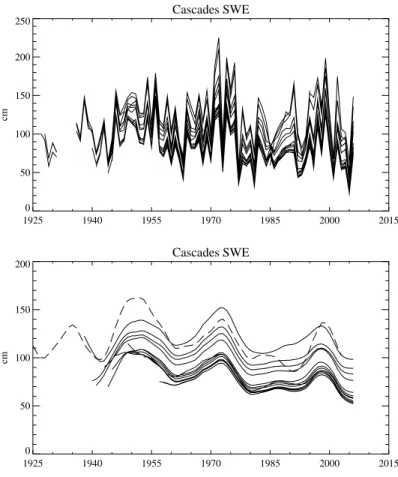
If missing data remain, the next-best-correlated snow course is used, and so on. The full set of regionally averaged time series is shown in Fig. 6. As each snow course is added it changes the average SWE, as suggested in Fig. 4b, largely as a function of elevation of the new snow course. Additions beyond about 1950 make little difference, as suggested also by Fig. 4b. Smoothing the time series (Fig. 6b)

15

clarifies the differences among the curves and also shows three interdecadal peaks in SWE, centered on about 1952, 1973, and 1998, with low points in the 1980s and early 1990s, similar to the VIC results repeated from Fig. 3a. Despite the fact that 2006 was a relatively good year for SWE, the very low years of 2001 and 2005 mean that the smoothed time series all end in a dip, which lies below the previous dip in around 1980

20

dominated by the very snow-poor years of 1977 and 1981 and other below-average years around that time. The ranking of snowiest or least snowy years, too, depends on which curve is chosen; for the 1938 curve the snowiest years are 1973, 1976, and 1956 (quite different from VIC), whereas for the 1956 curve the snowiest years are 1956, 1973, and 1999. Clearly any results derived from these regionally averaged time

25

series will depend on judicious choice of time series for further analysis.

We now explore the correspondence of linear fits between VIC and observations for different starting points (Table 3). Each entry shows the trend from the starting

(12)

HESSD

4, 2073–2110, 2007

Printer-friendly Version Interactive Discussion year to 2003 (the last year of the VIC simulation); the observational estimates are

for a changing mix of snow courses up to 1960. Most mid-century starting points yield a trend around –25% for observations and VIC, with a range of about –15% to –35%. Observed and VIC trends are within about 6% for starting points between 1945 and 1956; before 1945, the dearth of low-elevation snow courses affects the observed

5

trends, as would be expected from Fig. 4. It is less clear why the trends diverge for starting points beyond the late 1950s, perhaps land use change (encroachment of forests into snow courses). Trends are statistically significant (i.e. the 95th percentil estimate of the trend is negative) for observations for starting points between 1945 and 1954, and for VIC only between 1942 and 1950. The 5th percentile estimates

10

are mostly in the –35% to –55% range for observed starting points between 1942 and 1974, and for all VIC starting points between 1916 (not shown in the table) and 1974. Trends are generally positive, but not significant, for starting points after 1975.

With the goal of characterizing the variability over as long a time as possible without too severely underemphasizing low elevations, we use the time series starting in 1944.

15

From Table 3 it is clear that this is a fairly conservative estimate of the trends. 5.1 Regression analysis with temperature and precipitation

Complementing the analysis of the temperature-only VIC simulation presented in Sec-tion 4, we use empirical relaSec-tionships between 1 April SWE from each snow course and reference time series for temperature and precipitation in November through March,

20

roughly as in Mote (2006). For this analysis through 2006, US Historical Climate Network (USHCN). USHCN data were not available for 2006, so instead we use the Climate Division data for Washington Climate Division 4 (west slopes Cascades and foothills). As a first step in understanding the linear relationships between SWE and the climate variables, we show in Fig. 7 the correlations between 1 April SWE and

Nov-25

Mar mean temperature and precipitation, for different periods of analysis. Note that, consistent with Fig. 4 and the sensitivity of SWE at lower elevations to temperature, the correlation of regionally averaged SWE with precipitation drops somewhat and the

(13)

HESSD

4, 2073–2110, 2007

Printer-friendly Version Interactive Discussion correlation with temperature changes substantially from –0.3 to about –0.5. Next, the

climate data are used in multiple linear regression to estimate the regionally averaged snowpack for the regionally averaged time series of 1 April SWE since 1944. Regres-sion analysis against November–March precipitation and temperature is performed, as in Mote (2006):

5

SWE(t)=SWE0+ aTT(t) + aPP(t) + ε(t)

where SWE(t) is the 1 April SWE in year t, SWE₀ is the mean SWE, a_T and a_Pare the regression coefficients for temperature and precipitation respectively, and T(t) and P(t) are the values of temperature and precipitation in year t, and finally ε(t) is the residual. We can then also define S(t)=SWE0+aTT(t) + aPP(t), that is, the time series

10

generated directly from the climate data. Figure 8 shows SWE(t) and the resulting S(t) for the time series starting in 1944. The correlation between the two is 0.88, and the correspondence is obviously quite good in most years, though the trend in S(t) is substantially less than observed for a number of possible reasons (mainly that when variance is partitioned between a deterministic and a stochastic component, the

15

regressed extreme values tend to be less extreme and the slope of the fitted trend is consequently also reduced). There may also be some errors in the long-term trends in the climate division data; this calculation could be redone using USHCN stations in and near the Cascades, augmented for the most recent years using other data.

Using the regression approach permits a separation of the effects of temperature

20

SWE0+aTT(t) and precipitation SWE0+aPP(t) (Fig. 9). The two contributions sum to

the –12 cm in Fig. 8, though the percentage changes do not sum since they are com-puted relative to the value in 1944 for each linear fit, which is somewhat different. This analysis shows that to first order the long-term change is a result of warming, with precipitation adding noise that makes the trend detection more difficult, especially on

25

shorter time periods (see Fig. 3 and Table 3). We return to this subject below, where we examine the output of the simulation with the hydrology model. For the 1956–2006 time series (not shown), the observed decline is 27%, the trend in S(t) is –15%, the trend in a_PP is 0cm or 2% and the trend in a_TT is –5 cm or –17%. Hence, even for

(14)

HESSD

4, 2073–2110, 2007

Printer-friendly Version Interactive Discussion these fairly different starting points the results are similar: the trend is dominated by

a_TT(t).

5.2 Further distinguishing roles of temperature and precipitation

The ratio of 1 April SWE over precipitation (Fig. 10) shows what fraction of precipitation falling from November through March remains on the ground on 1 April, what we might

5

call the storage efficiency; that fraction has declined by 28% for observations and by 33% for VIC. Note that because the precipitation measurements come from weather stations, which are almost all located at low elevations where less precipitation falls, the actual precipitation was multiplied by 1.5 to reflect high-elevation enhancement of precipitation (this factor does not affect the computed trends). Storage efficiency was

10

worst for 2005, when much of the winter precipitation fell in three warm wet storms in what was otherwise not an exceptionally warm winter (Fig. 9).

We now show yet another way to examine the data with a view to determining whether warming has played a role in the observed changes. Recognizing that the fun-damental pattern of change in SWE in simulations of warming is a pronounced loss at

15

lower elevations, we use the same set of snow courses from 1944 as in Figs. 6 through 9, and construct time series of average SWE at elevations above 1200 m (“high”) and below 1200 m (“low”). The ratio of low to high elevation SWE is shown in Fig. 11, along with a linear fit. The slope parameter is statistically significant.

5.3 Area-weighting with elevation

20

In the foregoing analysis, time series at the various snow courses were combined by simple linear averaging. The area in each elevation band, however, decreases with elevation, so that even though low elevations have relatively little SWE per unit area (Fig. 3), they hold a large total quantity of snow. In order to estimate the importance of this effect, we construct elevation bands at 60 m vertical intervals, based on National

25

Geophysical Data Center 2-min etopo2 digital elevation for the Washington Cascades. 2085

(15)

HESSD

4, 2073–2110, 2007

Printer-friendly Version Interactive Discussion The hypsometric (cumulative area-altitude) relationship is shown in Fig. 12a along with

the altitudes of the elevation bands containing snow courses used in constructing the 1944–2006 time series shown in Figs. 6b–10. In Fig. 12b, the mean SWE from 1944 to 2006 at each snow course is multiplied by the area in that elevation band, and the resulting profile is interpolated to the elevation bands in which there are no snow

5

courses, then smoothed slightly. The median elevation is only 640 m, and half the SWE is found at elevations below 1025 m, which is represented by only four snow courses for the 1944–2006 time series (Table 1). Fully 90% of the snow on 1 April is found below 1600 m.

Using the area-weighting represented in Fig. 12b, we construct another time series

10

of regionally averaged 1 April SWE (Fig. 13). The strong weighting of the lower eleva-tions, where observed declines have been larger, produces a much larger linear trend, –35% over the 1944–2006 period, than in the unweighted time series (–24%, Fig. 8). Furthermore, it brings the observed trend exactly into line with the VIC trend over the 1944–2003 period of the VIC simulation.

15

6 Discussion and conclusions

When observations are weighted by the area of each elevation band, there is a re-markable congruence between observed and modeled estimates of regionally aver-aged SWE (Fig. 13). This is all the more remarkable because the point measurements of the observations and the gridded values of the model are fundamentally different

20

quantities, and furthermore the observations are potentially affected by a different set of time-varying biases (e.g., land cover change). Both the observationally derived and modeled estimates of total 1 April SWE have strengths and weaknesses. The model-ing produces robust spatially distributed estimates of SWE and the resultmodel-ing streamflow agrees well with observations, as does the simulated snow for roughly three-quarters of

25

the observed snow courses; on the other hand, VIC requires interpolated temperature and precipitation which may not always accurately reflect the daily values experienced

(16)

HESSD

4, 2073–2110, 2007

Printer-friendly Version Interactive Discussion in the remote mountains. The observed values are actual measurements but may be

influenced by site changes like canopy growth, and their spatial distribution is so sparse that areally averaged estimates are sensitive to choices about which snow courses to include. Such choices are especially important with respect to elevation, since (1) a great deal of snow on 1 April lies at relatively low elevations that are represented by a

5

very few snow courses and (2) long-term warming trends disproportionately affect low elevation snow (Fig. 5).

The smooth curves in Figs. 3 and 6 emphasize that there is substantial variability in 1 April SWE on timescales longer than several years. During the period of adequate instrumental coverage (1944–2006) three relatively snowy periods have occurred; in

10

the observations, each of these had a slightly lower peak than the last. In the VIC simulation, all three had roughly the same peak value. This difference is reflected also in the larger negative linear trend in the observations than in the VIC simulation over this time period and in the median difference between observed and VIC trends at individual locations over the 1950-97 period of analysis (Table 2). Considerable further

15

analysis will be required to elucidate the reasons for the differences in trends between model and observations.

Within a decade or so of 1955, selection of starting date does not greatly influence the linear declines computed from observations. The linear decline of 1 April SWE with ending point 2006 and from starting points between 1916 and 1970, calculated

20

either with VIC data or observations (the latter starting no earlier than 1944 to ensure adequate sampling of lower elevations), is roughly –15% to –34% and mostly around –25% (Table 3). Area-weighting the observations produces larger declines. For most of the mid-century starting points the trend in observed regionally averaged 1 April SWE is statistically significant. The drawback of using linear fits is that they obscure

25

interesting and significant features like the local maximum in SWE in the late 1990s. Fluctuations and trends in temperature and precipitation play distinct roles in the be-havior of these time series. Rising temperatures have clearly dominated in determining the regionally averaged trend in SWE over periods longer than about 30 years, as is

(17)

HESSD

4, 2073–2110, 2007

Printer-friendly Version Interactive Discussion evident in (a) the VIC simulation with fixed precipitation (Fig. 3b); (b) the regression

analysis (Fig. 9); (c) the declining “storage efficiency” (Fig. 10); (d) the strong depen-dence of trends on elevation (Fig. 5); and (e) the declining ratio of low elevation to high elevation snowpack. Precipitation produces much of the interannual variability but plays little role in trends except over short time periods (say, post-1970), and linear

5

trends in precipitation are not statistically significant over any period in contrast to those of temperature.

Further interpretation is required though. What is one to make of the positive (but not significant) trends in SWE since the early 1970s? What roles have Pacific decadal variability and human-induced global warming played in these changes?

10

Before answering these questions, we first note that the Pacific Decadal Oscillation (Mantua et al., 1997) was predominantly in one phase from 1945 to 1976 and in an-other phase from 1977 to perhaps 1997, with ambiguous phase since then, and that the period since 1997 (the past decade). We also note that with a declining storage efficiency caused by rising temperatures, the extremely high seasonal precipitation in

15

1997 and 1999, which helped make the most recent 10-year period the wettest period in the instrumental record and produced the peak in the smooth curve in Figs. 3 and 6, only managed to raise 1 April SWE to about half the value of the ∼1950 peak in the observed estimate, though they are closer in the VIC simulation.

We propose and test three hypotheses to answer these questions about

interpre-20

tation; these hypotheses each have corrolaries about future variability of Cascades SWE.

– Hypothesis 1: the variability and trends in SWE can be largely explained by Pacific

decadal variability. Table 3 can be interpreted as showing that the significant trends found for starting points between 1945 and 1954 depend entirely on the

25

1977 PDO regime shift.

– Corollary 1: Future variability in SWE is unpredictable but will vary around the

long-term mean.

(18)

HESSD

4, 2073–2110, 2007

– Hypothesis 2: Human-induced global warming in the Northwest includes large

increases in winter precipitation that have canceled the influence of warming dur-ing the period when human influence on global climate emerged, i.e. since the mid-1970s.

– Corollary 2: A human influence on Cascades SWE will be difficult to detect

be-5

cause trends in precipitation will continue to cancel trends in temperature.

– Hypothesis 3: a long-term decline in 1 April SWE driven by warming is detectable,

but has been partly obscured in the past decade or so by random fluctuations of precipitation.

– Corollary 3: future SWE will decline, especially at low elevations.

10

Tools used to test these hypotheses include time series analysis, spatial analysis, and modeling of future SWE with VIC.

1) The subject of natural variability and its connection to variations and trends in western snowpack has been examined by Mote (2006), Stewart et al. (2005), and Clark et al. (2001). Mote (2006) regressed individual time series of SWE in the West

15

on the North Pacific Index, an atmospheric index sensitive to both ENSO and PDO variability, and found that 10–60% of trend in SWE at snow courses in the Pacific Northwest could be explained by the North Pacific Index (an indicator of the strength of the Aleutian Low that responds both to the PDO and to ENSO), a larger fraction than for the PDO index itself. Response to NPI is characterized by an out-of-phase

20

relationship between the PNW and the Southwest, and the strong positive trends in precipitation in the Southwest since 1950 (chiefly the result of a severe drought in the 1950s and early 1960s) overwhelmed the influence of rising temperatures there, producing positive trends in SWE at most sites.

In this hypothesis, the negative PDO phase that prevailed from 1945 to 1976

pro-25

duced the high values of SWE during that period, the positive phase of the PDO that prevailed from 1977 to 1997 produced low values of SWE, and a negative PDO phase

(19)

HESSD

4, 2073–2110, 2007

Printer-friendly Version Interactive Discussion beginning in 1999 produced high values of SWE observed since then. However, three

significant problems with this hypothesis emerge. First, the phase of the PDO is not accurately represented by constant values that change sign every few decades, and in particular the PDO index has not shown a clear preference for positive or negative values in the past 10 years, nor a strong correspondence to PNW SWE. Second, even

5

with the NPI or PDO regressed out of the time series of SWE, a substantial negative trend in 1 April SWE remains and in fact becomes statistically significant. We cor-relate and regress the 1944–2006 time series of 1 April SWE shown in Fig. 6 with November–March NPI: the correlation is 0.53, so NPI plays a significant role in inter-annual variability, but with NPI regressed out the trend changes only from –18.6% to

10

–14.6% (Figure 14). The coefficient of variation is cut in half from 0.28 to 0.15 which is why the trend becomes statistically significant. Third, if the period since 1997 or 1999 has been a negative phase PDO it does not explain the very low snow years of 2001 and 2005, nor the much lower storage efficiency for most years since 1997.

2) One could test the second hypothesis by testing for an emerging human influence

15

on temperature and precipitation separately. A useful metric for emerging human influ-ence is the logarithm of global CO₂, a rough approximation of the radiative forcing and hence the climatic influence of human activity. Regression of ln(CO2) on temperature

produces a fairly large coefficient, explaining much of the observed trend. However, for precipitation the regression is close to zero. This hypothesis also is inconsistent with

20

the twenty scenarios of Northwest climate produced under the auspices of the IPCC and analyzed by Mote et al. (2005b), which suggest only modest changes (a few %) in winter precipitation in response to rising greenhouse gases. This is consistent with evidence in the literature that at least on the scale of the West a human influence on air temperature can be detected (e.g., Stott, 2003) but also that neither globally nor

25

regionally can a human influence on precipitation be detected (Gillett et al., 2004). In simulations with the VIC hydrology model, even large increases in winter precipitation were not sufficient to offset losses in the Cascades associated with warming (e.g., Hamlet and Lettenmaier, 1999).

(20)

HESSD

4, 2073–2110, 2007

Printer-friendly Version Interactive Discussion 3) The third hypothesis is supported by several lines of evidence. The time

se-ries analysis presented above suggests that precipitation behaves like random noise. Exceptionally high values of winter precipitation in 1997 and 1999 made short-term trends (early 1970s to present) near-zero or even positive, though none of these are statistically significant. Indeed, the local maximum in the late 1990s was followed by

5

exceptionally low values in 2001 and 2005 which produce a sharp dip in the smoothed curves (Figs. 3b and 6). A second line of evidence concerns the spatial signal of warm-ing, namely the elevation-dependent decline in snowpack, which clearly has emerged: see Figs. 5 and 11. Modeling studies (e.g., Hamlet and Lettenmaier 1999, Hamlet et al., 2005) clearly indicate that an elevation-dependent decline in snowpack is a robust

10

response to regional warming under anthropogenic influence for both past and future changes in temperature and precipitation combined. This is not to say that the ob-served changes in SWE can be conclusively linked to rising greenhouse gases; such attribution on the spatial scale of the Cascades is not yet possible. Furthermore, it is not yet clear what role greenhouse gases may have played in changes in the NPI;

15

some studies suggest that the observed changes in the NPI may themselves be re-lated to anthropogenic climate change, in which case “removing” the NPI as was done in testing Hypothesis 1 may remove both anthropogenic and natural factors.

None of these hypotheses is completely satisfactory, but it is clear that warming has had a significant effect on Cascades snowpack especially at lower elevations where

20

SWE has declined dramatically. These declines, while influenced by Pacific decadal variability, are dominated by warming trends largely unrelated to Pacific climate vari-ability and strongly congruent with trends expected from rising greenhouse gases.

Acknowledgements. Snow course measurements provide unique climate records of the moun-tainous regions of the West, and we wish to thank heartily the dedicated snow surveyors of

25

decades past and of today for making the measurements described herein, and NRCS for pro-viding the data. We also thank R. Norheim for constructing the map in Fig. 1, and D. Hartmann, R. Wood, H. Harrison, D. Lettenmaier, K. Redmond, and N. Mantua for helpful comments on an earlier version of this manuscript. This publication was funded by the Joint Institute for the Study of the Atmosphere and Ocean (JISAO) at the University of Washington under NOAA

30

(21)

HESSD

4, 2073–2110, 2007

Cooperative Agreement No. NA17RJ1232, Contribution #1411.

References

Cherkauer, K. A. and Lettenmaier D. P.: Simulation of spatial variability in snow and frozen soil, J. Geophys. Res., 108, 8858, doi:10.1029/2003JD003575, 2003.

Cleveland, W. S.: Visualizing Data, Hobart Press, Summit, N.J., 1993.

5

Gillett, N. P., Weaver, A. J., Zwiers, F. W., and Wehner, M. F.: Detection of volcanic influence on global precipitation, Geophys. Res. Lett., 31(12), L12217, doi:10.1029/2004GL020044, 2004b.

Hamlet, A. F. and Lettenmaier, D. P.: Production of temporally consistent gridded precipitation and temperature fields for the continental U.S., J. Hydrometeorology, 6(3), 330–336, 2005.

10

Hamlet, A. F., Mote, P. W., Clark, M. P., and Lettenmaier, D. P.: Effects of temperature and precipitation variability on snowpack trends in the western U.S., J. Climate, 18, 4545–4561, 2005.

Karl, T. R., Williams Jr., C. N., Quinlan, F. T., and Boden, T. A.: United States Historical Cli-matology Network (HCN) Serial Temperature and Precipitation Data, Environmental Science

15

Division, Publication No. 3404, Carbon Dioxide Information and Analysis Center, Oak Ridge National Laboratory, Oak Ridge, TN, 389 pp., 1990.

Lemke, P., Ren, J., Alley, R. B., Allison, I., Carrasco, J., Flato, G., Fujii, Y., Kaser, G., Mote, P., Thomas, R. H., and Zhang, T., Observations: Changes in Snow, Ice and Frozen Ground. Chapter 4 in: Climate Change 2007: The Physical Science Basis. Contribution of

Work-20

ing Group I to the Fourth Assessment Report of the Intergovernmental Panel on Climate Change, edited by: Solomon, S., Qin, D., Manning, M., Chen, Z., Marquis, M., Averyt, K. B., Tignor, M., and Miller, H. L., Cambridge University Press, Cambridge, United Kingdom and New York, NY, USA, 2007.

Liang, X., Lettenmaier, D. P., Wood, E. F., and Burges, S. J.: A simple hydrologically based

25

model of land surface water and energy fluxes for general circulation models, J. Geophys. Res., 99(D7), 14 415–14 428, 1994.

Mote, P. W.: Climate-driven variability and trends in mountain snowpack in western North Amer-ica, J. Climate, 19, 6209–6220, 2006.

(22)

HESSD

4, 2073–2110, 2007

Mote, P. W., Hamlet, A. F., Clark, M. P., and Lettenmaier, D. P.: Declining mountain snowpack in western North America, Bull. Am. Meteorol. Soc., 86, 39–49, 2005.

Regonda S., Rajagopalan B., Clark M., and Pitlick J.: Seasonal cycle shifts in hydroclimatology over the Western US, J. Climate, 18, 372–384, 2005.

Salath ´e, E. P., Mote, P. W., and Wiley, M. W.: Considerations for selecting

downscal-5

ing methods for integrated assessments of climate change impacts, Intl. J. Climatol., doi:10.1002/joc.1540, 2007.

Stott, P. A.: Attribution of regional-scale temperature changes to anthropogenic and natural causes, Geophys. Res. Lett., 30, 1728, doi:10.1029/2003GL017324

10

(23)

HESSD

4, 2073–2110, 2007

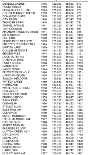
Table 1. Locations and starting year of snow courses used in this study, sorted by elevation.

“AM” refers to aerial markers, where snow depth is estimated from aerial photos of a snow stake and SWE is inferred from snow depth.

name started longitude latitude elev (m) MEADOW CABINS 1945 120.933 48.583 579 ROCKY CREEK 1959 121.800 48.683 640 BEAVER CREEK TRAIL 1944 121.200 48.833 670 S.FORK THUNDER CREEK 1959 121.667 48.600 670 DOMMERIE FLATS 1939 121.067 47.233 670 CITY CABIN 1948 121.517 47.317 728 THUNDER BASIN 1948 120.983 48.517 731 TUNNEL AVENUE 1941 121.350 47.317 746 TOATS COULEE 1959 119.733 48.850 867 AHTANUM RANGER STATION 1941 121.017 46.517 945 MT. GARDNER 1959 121.567 47.367 1006 FISH LAKE 1943 121.567 47.517 1027 SCHREIBERS MEADOW 1959 121.817 48.700 1036 FREEZEOUT CREEK TRAIL 1944 120.950 48.950 1067 MARTEN LAKE 1959 121.717 48.767 1097 OLALLIE MEADOWS 1945 121.450 47.383 1105 BEAVER PASS 1944 121.250 48.883 1121 DOCK BUTTE AM 1959 121.800 48.633 1158 STAMPEDE PASS 1943 121.333 47.283 1176 RUSTY CREEK 1943 119.867 48.533 1219 SATUS PASS 1957 120.683 45.983 1228 SASSE RIDGE 1944 121.050 47.367 1280 BLEWETT PASS NO. 2 1946 120.683 47.350 1301 UPPER WHEELER 1959 120.367 47.283 1341 SALMON MEADOWS 1938 119.833 48.667 1371 WATSON LAKES 1959 121.583 48.667 1371 HURRICANE 1949 123.533 47.967 1371 WHITE PASS (E. SIDE) 1953 121.383 46.633 1371 COX VALLEY 1959 123.483 47.967 1371 PARK CREEK RIDGE 1928 120.917 48.450 1402 BUMPING RIDGE 1953 121.333 46.817 1402 RAINY PASS 1930 120.717 48.567 1457 CHEWELAH 1958 117.583 48.283 1501 STEMILT SLIDE 1959 120.383 47.283 1524 EASY PASS AM 1959 121.433 48.867 1585 DEER PARK 1949 123.250 47.950 1585 BOYER MOUNTAIN 1946 117.433 48.200 1600 LITTLE MEADOWS AM 1927 120.900 48.200 1608 CAYUSE PASS 1940 121.533 46.867 1615 JASPER PASS AM 1959 121.400 48.783 1646 PARADISE PILLOW 1940 121.717 46.800 1676 MUTTON CREEK NO. 1 1938 119.867 48.667 1737 DEVILS PARK 1950 120.850 48.750 1798 LYMAN LAKE 1928 120.917 48.200 1798 GREEN LAKE 1941 121.167 46.550 1829 CORRAL PASS 1940 121.467 47.017 1829 MINERS RIDGE 1928 120.983 48.167 1890 HARTS PASS 1941 120.650 48.717 1981 CLOUDY PASS AM 1927 120.917 48.200 1981 2094

(24)

HESSD

4, 2073–2110, 2007

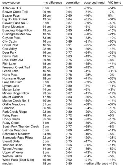
Table 2. Comparison of VIC and observed 1 April SWE, 1950–1997.

snow course rms difference correlation observed trend VIC trend Ahtanum R.S. 8 cm 0.71 –39% –54% Beaver Creek Trail 29 cm 0.64 –51% –7% Beaver Pass 26 cm 0.60 –46% 0% Big Boulder Creek 13 cm 0.84 –31% –34% Blewett Pass No. 2 8 cm 0.87 –39% –43% Boyer Mountain 34 cm 0.84 –3% –33% Bumping Ridge Pillow 15 cm 0.85 –14% –15% Bunchgrass Meadow 13 cm 0.83 –20% –21% Cayuse Pass 63 cm 0.78 –33% –10% City Cabin 16 cm 0.89 –81% –65% Corral Pass 16 cm 0.91 –25% –29% Cox Valley 22 cm 0.76 –30% –18% Deer Park 16 cm 0.77 –64% –35% Devils Park 19 cm 0.83 –13% –15% Dock Butte AM 39 cm 0.75 –35% –6% Fish Lake 18 cm 0.86 –35% –44% Freezout Creek Trail 28 cm 0.66 –45% –7% Green Lake 16 cm 0.78 +2% +11% Harts Pass 18 cm 0.78 –28% –2% Hurricane Ridge 18 cm 0.80 –71% –35% Lake Cle Elum 9 cm 0.89 –89% –65% Lyman Lake 27 cm 0.80 –6% –11% Marten Lake 44 cm 0.68 –5% +3% Miners Ridge Pillow 23 cm 0.87 –11% –19% Mount Gardner 17 cm 0.83 –56% –50% Mutton Creek No. 1 10 cm 0.76 –30% –14% Olallie Meadows 31 cm 0.84 –58% –37% Paradise 36 cm 0.84 –24% –10% Park Creek Ridge 22 cm 0.80 –20% –20% Rainy Pass 18 cm 0.72 –29% –5% Rocky Creek 25 cm 0.78 –23% –15% Rusty Creek 4 cm 0.82 –56% –25% South Fork Thunder Creek 9 cm 0.77 –68% –8% Salmon Meadows 6 cm 0.80 –40% –14% Schreibers Meadow 34 cm 0.76 –40% –5% Stampede Pass Pillow 22 cm 0.84 –20% –28% Stemilt Slide 8 cm 0.75 –17% –17% Thunder Basin 42 cm 0.56 –36% –11% Tunnel Avenue 14 cm 0.87 –56% –52% Upper Wheeler 9 cm 0.64 –43% –17% Watson Lakes 38 cm 0.69 –34% –5% White Pass (East Side) 16 cm 0.92 –21% –15% median 18 cm 0.80 median difference –15%

(25)

HESSD

4, 2073–2110, 2007

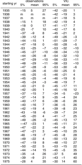
Table 3. Linear trend (%) from starting year to 2003 for observations and VIC, with 5% and

95% confidence levels of the trend.

starting yr _5%observations_mean _95% _5% _meanVIC _95%

1935 –15 5 27 –42 –20 1 1936 m m m –42 –19 3 1937 m m m –41 –18 5 1938 –15 1 18 –42 –19 4 1939 –18 0 17 –41 –17 7 1940 -25 -7 10 –42 –17 6 1941 –37 –9 8 –45 –21 2 1942 –39 –12 4 –49 –26 –3 1943 –44 –15 1 –51 –29 –7 1944 –47 –18 0 –50 –28 –5 1945 -53 –25 –7 –53 –32 –10 1946 –45 –27 –10 –56 –34 –13 1947 –44 –26 –8 –54 –32 –10 1948 –47 –29 –10 –56 –33 –11 1949 –48 –29 –11 –56 –33 –10 1950 –47 –28 –9 –53 –30 –6 1951 –46 –26 –6 –50 –25 0 1952 –45 –25 –5 –46 –21 4 1953 –45 –25 –4 –46 –19 6 1954 –45 –24 –3 –46 –19 7 1955 –43 –21 0 –45 –17 11 1956 –42 –20 1 –45 –16 12 1957 –37 –15 7 –34 –5 –23 1958 –37 –14 9 –35 –4 24 1959 –40 –17 6 –36 –6 26 1960 –40 –16 7 –36 –5 26 1961 –42 –19 4 –39 –8 23 1962 -43 –18 -6 –39 –7 24 1963 –45 –20 4 –41 –7 25 1964 –49 –26 –2 –45 –13 17 1965 —47 –23 1 –45 –11 21 1966 –47 –22 2 –44 –9 24 1967 –47 –21 3 –45 –10 25 1968 -46 –19 -7 –45 –8 28 1969 –49 –22 4 –50 –13 22 1970 –47 –19 8 –48 –10 27 1971 –50 –22 5 –53 –15 22 1972 –44 –14 15 –45 –5 35 1973 –35 –4 26 –37 5 49 1974 –39 –9 21 –43 –1 40 1975 –26 4 35 –30 14 60 2096

(26)

HESSD

4, 2073–2110, 2007

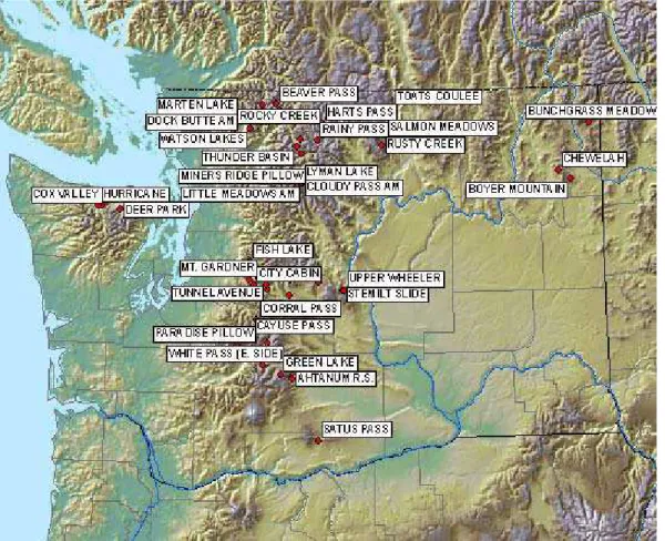
Fig. 1. Map of Washington’s Cascades and Olympics with snow course locations indicated.

(27)

HESSD

4, 2073–2110, 2007

Printer-friendly Version Interactive Discussion WA CAYUSE PASS o1615m v -16m

1950 1960 1970 1980 1990 2000

rmsd 63cm corr 0.78 obs tr -33% VIC tr -10% 0 100 200 300 400 WA CITY CABIN o 728m v 161m 1950 1960 1970 1980 1990 2000

rmsd 16cm corr 0.89 obs tr -81% VIC tr -65% 0 20 40 60 80 100 120

WA CORRAL PASS o1829m v -510m

1950 1960 1970 1980 1990 2000

rmsd 16cm corr 0.91 obs tr -25% VIC tr -29% 0 50 100 150 200 250

WA CORRAL PASS PILLOW o1829m v -461m

1950 1960 1970 1980 1990 2000

rmsd 16cm corr 0.81 obs tr -20% VIC tr -24% 0

50 100 150

WA COX VALLEY o1371m v -141m

1950 1960 1970 1980 1990 2000

50 100 150 200

WA DEER PARK o1585m v -588m

1950 1960 1970 1980 1990 2000

WA DEVILS PARK o1798m v -739m

1950 1960 1970 1980 1990 2000

50 100 150 200

WA DOCK BUTTE AM o1158m v -73m

1950 1960 1970 1980 1990 2000

WA FISH LAKE o1027m v 97m

1950 1960 1970 1980 1990 2000

50 100 150 200

WA FISH LAKE PILLOW o1027m v 45m WA FREEZEOUT CR. TR. o1067m v -31m WA GREEN LAKE o1829m v -383m Figure 2. Observed (o) and VIC simulated (+) April 1 SWE at nine of the snow courses in Wash

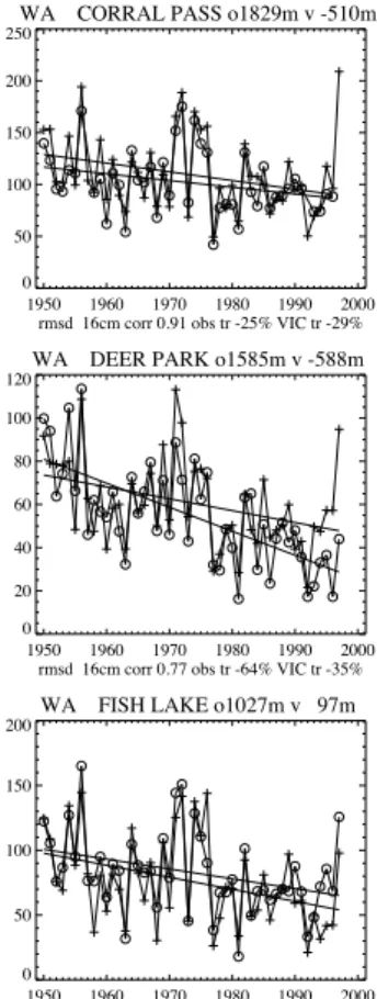
Fig. 2. Observed (o) and VIC simulated (+) 1 April SWE at nine of the snow courses in

Wash-ington for 1950–1997 (or shorter). Each frame includes statistics about the elevation of the snow course (o1615m for Cayuse Pass), the difference in elevation between the VIC grid cell and the snow course (positive means VIC higher), root mean square (rms) difference between simulated and observed SWE, correlation, observed trend, and trend simulated by VIC. Data

(28)

HESSD

4, 2073–2110, 2007

Printer-friendly Version Interactive Discussion VIC swe 1910 1930 1950 1970 1990 2010 year 20 40 60 80 100 120 140 160 cm 1950-2003: -31% 1916-2003: -16%

VIC swe, fixed precipitation

1910 1930 1950 1970 1990 2010 year 20 40 60 80 100 120 140 cm 1950-2003: -20% 1916-2003: -13%

Fig. 3. 1 April SWE simulated by VIC, averaged over the domain of the Cascades and Olympics

for the full simulation (top) and for a temperature-only simulation (bottom), with linear fits and loess smoothing for the time periods indicated.

(29)

HESSD

4, 2073–2110, 2007

Washington snow courses

1925 1935 1945 1955 1965 0 10 20 30 40 50 60 N um be r 1000 1250 1500 1750 2000 E le va ti on, m et ers 0 50 100 150 200 250 300 long-term mean SWE, cm 0 500 1000 1500 2000 E le va ti on, m

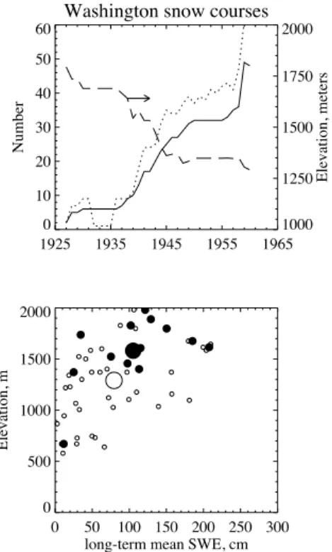
Fig. 4. Elevation, and hence temperature sensitivity, of the full set of snow courses for the

Washington Cascades and Olympics changes over time. Early snow courses substantially un-dersampled middle and low elevations. (a) Number of snow courses reporting 1 April data (dotted line) for each year; for each starting year, number of snow courses at least 80% com-plete over the period of record (thick solid line), and their mean elevation (long dashed line, right-hand axis). Note how the early snow courses were few and were at higher elevation. (b) Scatterplot of mean 1 April SWE against elevation of all snow courses (open circles) and of snow courses available in 1940 (solid circles). The mean value for each set is indicated by the large circles; mean SWE changes by 26 cm and the mean elevation by 290 m.

(30)

HESSD

4, 2073–2110, 2007

Printer-friendly Version Interactive Discussion Trends since 1940 (1930, +) -120 -80 -40 0 40 Percent change 500 1000 1500 2000 E le va ti on, m Trends since 1950 -120 -80 -40 0 40 Percent change 500 1000 1500 2000 E le va ti on, m Trends since 1960 -120 -80 -40 0 40 Percent change 500 1000 1500 2000 E le va ti on, m Trends since 1970 -120 -80 -40 0 40 Percent change 500 1000 1500 2000 E le va ti on, m

Fig. 5. Dependence of linear trends in 1 April SWE on elevation, for different starting years

through the end of the record (plus symbols in the first frame indicate trends from 1930). The pronounced and consistent dependence of trends on elevation is an indication of the role of warming trends (see Mote; 2003, 2006; Mote et al.; 2005; Hamlet et al., 2005; Regonda et al., 2005).

(31)

HESSD

4, 2073–2110, 2007

Printer-friendly Version Interactive Discussion Cascades SWE 1925 1940 1955 1970 1985 2000 2015 0 50 100 150 200 250 cm Cascades SWE 1925 1940 1955 1970 1985 2000 2015 0 50 100 150 200 cm

Fig. 6. Twenty-six different time series of regionally averaged SWE for the Washington

Cas-cades are constructed by including all snow courses available by the date indicated. The bot-tom panel shows the data, smoothed (see appendix for details). Thick dashed curve shows VIC values from Fig. 3.

(32)

HESSD

4, 2073–2110, 2007

Correlations, Apr 1 SWE and NDJFM T and P

1930 1940 1950 1960 1970 Starting year 0.20 0.30 0.40 0.50 0.60 0.70 0.80 0.90 inches - corr(SWE,T) 2 3 4 5 6 7 Temperature, o_C 0 50 100 150 SWE, cm 40 60 80 100 120 140 160 Precipitation, cm 0 50 100 150 SWE, cm

Fig. 7. Top panel: correlation between regionally averaged 1 April SWE and November–March

(top) precipitation and (bottom, negative) temperature for each starting year through 2006 (i.e., the 26 time series shown in Fig. 6 in which new snow courses are added through 1960; after that the time window simply shrinks). Note that, consistent with Figs. 4–5 and the sensitivity of SWE at lower elevations to temperature, the correlation of regionally averaged SWE with precipitation drops somewhat and the correlation with temperature changes substantially from –0.3 to about –0.5. Bottom two panels show scatterplots of 1 April SWE vs climate division 4 temperature (left) and precipitation (right), for the time series starting in 1944.

(33)

HESSD

4, 2073–2110, 2007

SWE, observed and reconstructed from T and P

1940 1950 1960 1970 1980 1990 2000 2010 20 40 60 80 100 120 140 160 obs:-24% reg:-13%

Fig. 8. For the 1944–2006 time series of 1 April SWE, the observed time series (trend –24%,

–25 cm) and fitted time series S(t) (trend –13%, or –12 cm; diamond symbols).

(34)

HESSD

4, 2073–2110, 2007

Printer-friendly Version Interactive Discussion SWE and precipitation

1940 1950 1960 1970 1980 1990 2000 2010 20 40 60 80 100 120 140 S W E , c m 50 75 100 125 150 P re ci p, c m P: 6cm, 5% SWE: 5cm, 6%

SWE and temperature

1940 1950 1960 1970 1980 1990 2000 2010 40 60 80 100 120 S W E , c m 2 3 4 5 6 7 T em p, oC T: 1.4o C SWE: -17cm, -18%

Fig. 9. Time series of (top) aPP(t), left axis and precipitation in cm, right axis; (bottom) aTT(t),

left axis and temperature (right axis, note inverted scale). Linear trends for each quantity are both graphed and printed, and the loess curve is shown as well.

(35)

HESSD

4, 2073–2110, 2007

Printer-friendly Version Interactive Discussion SWE / NDJFM precip 1940 1950 1960 1970 1980 1990 2000 2010 year 0 20 40 60 80 % -28% -33%

Fig. 10. “Storage efficiency”, the ratio of 1 April SWE to November–March precipitation, with

linear fit, for (top) observations 1944–2006 and (bottom) VIC simulation 1944–2003. The aver-age storaver-age efficiency in VIC is lower because the domain includes a lot of low-elevation grid points, but the percentage changes are similar.

(36)

HESSD

4, 2073–2110, 2007

Printer-friendly Version Interactive Discussion Cascades SWE 1940 1950 1960 1970 1980 1990 2000 2010 0 20 40 60 80 inches

Low elev / high elev

1940 1950 1960 1970 1980 1990 2000 2010 0.0 0.2 0.4 0.6 0.8

Fig. 11. Ratio of 1 April SWE at low-elevation (<1200m) snow courses to SWE at high-elevation

(>1200 m) snow courses. With the linear fit, the ratio has declined from 0.42 to 0.33 from 1944 to 2006; note also that in 2005 and 1981 the low elevations had less than 15% as much SWE as the high elevations. This metric is a good representation of the pattern expected from regional warming.

(37)

HESSD

4, 2073–2110, 2007

Area-elevation for Washington Cascades

0 20 40 60 80 100 % of area 250 500 750 1000 1250 1500 1750 2000 Elevation, m 0 20 40 60 80 100 % of snow 250 500 750 1000 1250 1500 1750 2000 Elevation, m

Fig. 12. Cumulative area (left) and SWE (right) as a function of elevation in thousands of feet,

for the Washington Cascades. In the left panel the asterisks indicate the 60-m elevation bands with at least one snow course. In the right panel the lines indicate the 50th and 90th percentiles.

(38)

HESSD

4, 2073–2110, 2007

Area-weighted Cascades SWE

1935 1950 1965 1980 1995 2010 0 50 100 150 cm obs: -28% VIC: -27%

Fig. 13. Regionally averaged 1 April SWE for observations (o) computed for the 1944–2006

snow courses using area-weighting and infilling of missing values with best-correlated time series, and VIC (v). The VIC values have been scaled to the mean observed SWE. Linear fits for observed (solid) and VIC (dashed) overlap.

(39)