Attribution of modeled atmospheric sulfate and SO₂ in the Northern Hemisphere for June?July 1997

HAL Id: hal-00296059

https://hal.archives-ouvertes.fr/hal-00296059

Submitted on 23 Oct 2006

HAL is a multi-disciplinary open access

archive for the deposit and dissemination of

sci-entific research documents, whether they are

pub-lished or not. The documents may come from

teaching and research institutions in France or

abroad, or from public or private research centers.

L’archive ouverte pluridisciplinaire HAL, est

destinée au dépôt et à la diffusion de documents

scientifiques de niveau recherche, publiés ou non,

émanant des établissements d’enseignement et de

recherche français ou étrangers, des laboratoires

publics ou privés.

the Northern Hemisphere for June?July 1997

C. M. Benkovitz, S. E. Schwartz, M. P. Jensen, M. A. Miller

To cite this version:

C. M. Benkovitz, S. E. Schwartz, M. P. Jensen, M. A. Miller. Attribution of modeled atmospheric

sulfate and SO2 in the Northern Hemisphere for June?July 1997. Atmospheric Chemistry and Physics,

European Geosciences Union, 2006, 6 (12), pp.4723-4738. �hal-00296059�

www.atmos-chem-phys.net/6/4723/2006/ © Author(s) 2006. This work is licensed under a Creative Commons License.

Chemistry

and Physics

Attribution of modeled atmospheric sulfate and SO

2

in the Northern

Hemisphere for June–July 1997

C. M. Benkovitz, S. E. Schwartz, M. P. Jensen, and M. A. Miller

Brookhaven National Laboratory, P.O. Box 5000, Upton, NY 11973, USA

Received: 16 January 2006 – Published in Atmos. Chem. Phys. Discuss.: 22 May 2006 Revised: 1 August 2006 – Accepted: 15 October 2006 – Published: 23 October 2006

Abstract. Anthropogenic sulfate aerosol is a major

contrib-utor to shortwave radiative forcing of climate change by di-rect light scattering and by perturbing cloud properties and to local concentrations of atmospheric particulate matter. Here we analyze results from previously published calcula-tions with an Eulerian transport model for atmospheric sul-fur species in the Northern Hemisphere in June–July, 1997 to quantify the absolute and relative contributions of spe-cific source regions (North America, Europe, and Asia) and SO2-to-sulfate conversion mechanisms (gas-phase,

aqueous-phase and primary sulfate) to sulfate and SO2 column

bur-dens as a function of location and time. Although mate-rial emitted within a given region dominates the sulfate and SO2column burden in that region, examination of time

se-ries at specific locations shows that material imported from outside can make a substantial and occasionally dominant contribution. Frequently the major fraction of these exoge-nous contributions to the sulfate column burden was present aloft, thus minimally impacting air quality at the surface, but contributing substantially to the burden and, by impli-cation, to radiative forcing and diminution of surface irradi-ance. Although the dominant sulfate formation pathway in the domain as a whole is aqueous-phase reaction in clouds (62%), in regions with minimum opportunity for aqueous-phase reaction gas-aqueous-phase oxidation is dominant, albeit with considerable temporal variability depending on meteorolog-ical conditions. These calculations highlight the importance of transoceanic transport of sulfate, especially at the western margins of continents under the influence of predominantly westerly transport winds.

Correspondence to: C. M. Benkovitz

(cmb@bnl.gov)

1 Introduction

Anthropogenic aerosols are thought to be influencing climate by offsetting the radiative forcing of greenhouse gases (Pen-ner et al., 2001; Ramaswamy et al., 2001; Bellouin et al., 2005) via scattering and absorption of radiation (direct ef-fect) and by enhancing the reflectivity and lifetimes of clouds (indirect effect). Aerosol forcing is strongest in the indus-trialized areas of North America, Europe, and Asia (Ra-maswamy et al., 2001). Solar radiation reaching the sur-face of the Earth has decreased discernibly during the past 50 years (Liepert, 2002; Stanhill and Cohen, 2001); these decreases also are more pronounced in industrialized areas. Atmospheric aerosols also contribute to deterioration of air quality in industrialized areas affecting human health and welfare. A major component of aerosols in these areas is sulfate resulting from the atmospheric oxidation of anthro-pogenically emitted sulfur dioxide (SO2)(U.S.

Environmen-tal Protection Agency, 2001). The long-range transport of anthropogenic sulfate aerosols (Perry et al., 1999; Piketh et al., 2002) suggests the need for quantifying the extent of the influence of source regions and source types on sulfate and SO2mixing ratios and column burdens.

A variety of approaches have been used to determine the influence of source regions and source types on the bur-dens of atmospheric trace species. Simulations using Eu-lerian models have been performed with and without emis-sions from certain source regions (Yienger et al., 2000); the influence of those source regions is estimated as the dif-ference in the atmospheric burden between the two simu-lations. This method is suitable provided removing the se-lected sources does not appreciably alter the chemistry of the species being studied, but for species such as sulfur and ni-trogen whose chemistry alters atmospheric concentrations of oxidant species this method may result in approximate esti-mates only. Lagrangian models that track emitted parcels in-dividually have been used to model regional transport

(Mal-COMPONENTS OF THE TRANSPORT AND TRANSFORMATION MODEL VERSION 2

OXIDANT

CONCENTRATIONS

Monthly average

with diurnal cycle

OH, HO₂, H₂O₂, O₃ Mozart (Brasseur et al)

TRANSPORT Advection Bott/Easter Vertical Turbulent Mixing

Convective Cloud Mixing Walcek-Taylor/Berkowitz

GAS Phase Chemistry SO2 + OH

DMS + OH DMS chem Yin/Seinfeld

HO2 + HO2

AQUEOUS Phase Chemistry SO2 + H2O2 SO2 + O3 IN CLOUD Activation: Proportional to LWVF, max 0.5 DRY DEPOSITION

Time, location dependent Wesely

WET DEPOSITION Exponential decay in cloud

EMISSIONS EDGAR/GEIA Anthro SO2, primary sulfate BNL/KETTLE/LISS Ocean DMS Lamb Land DMS, H2S BNL VOLCANOS SO2

SO

(Rate constants NASA, 1997)

MSA

SO

DMS

Derived fields: Kzz, air den.,

cloud param, geopot, vertical velocity

RESOLUTION

horizontal: 1O_x1O

27 vertical levels

Fig. 1. Schematic of the processes included in the Global Chemistry Model driven by observation-derived meteorology (GChM-O). Here,

BNL/Kettle/Liss, Brookhaven National Laboratory, Kettle et al. (1999), Liss and Merlivat (1986); Lamb (Bates et al., 1992); Horowitz (2003); Bott/Easter (Bott, 1989; Easter, 1993); Easter and Luecken (1988); Walcek-Taylor/Berkowitz (Walcek and Taylor, 1986); NASA (1997); Yin/Seinfeld (Yin et al., 1990a, b); Schwartz (1988); Wesely (Sheih et al., 1986; Wesely, 1989), and Benkovitz et al. (1994).

com et al., 2000). Concerns with this approach include rep-resentation of the interactions among species from multi-ple sources. Measurements coumulti-pled with air-mass back tra-jectory calculations have been used to determine potential source regions of the measured species (Jaffe et al., 1999; Martin et al., 2003; Perry et al., 1999; Allan et al., 2004). For example, Allan et al. (2004) presented an instance at Trinidad Head, California, in which appreciable non-seasalt sulfate was present in an airmass directly from the west that had had no discernible influence from North American sources. However this method is limited to the times and locations where measurements have been performed, and uncertainties and limitations in the back trajectory analyses grow quickly with time and may identify different source regions depend-ing on the type of back trajectory analysis performed. With varying degrees of uncertainty all these methods are able to qualitatively represent the influences of various source re-gions on the amount of material at receptor locations of in-terest; however, quantification of these influences is rarely possible and subject to large uncertainties.

Eulerian models with accurate representations of the sul-fur cycle and the ability to track sulsul-fur by source regions and source types are capable of more rigorous quantitative studies (Benkovitz et al., 1994; Graf et al., 1997; Rasch et al., 2000; Uno et al., 2003). Benkovitz et al. (1994) used an Eulerian sub-hemispheric chemical transport model with emissions labeled by source type (anthropogenic, biogenic) and source region (North America and Europe) to study the

sulfate and SO2 burdens for four seasonal six-week

peri-ods in 1986–1987. Sulfate concentrations and column bur-dens exhibited rich temporal and spatial structure related to existing meteorological patterns for each season. For the October-November 1986 simulation a pronounced variabil-ity was found in the contribution of the source regions to the sulfate burden over oceanic areas; over the mid north At-lantic the variation over a six-hour period in the fraction of the burden due to North American sources was between 25 and 58% and the variation in the fraction due to European sources was between 2 and 33%. Graf et al. (1997) carried out a five-year simulation with the Hamburg climate model European Centre Hamburg (ECHAM) global general circula-tion model (GCM) with a representacircula-tion of the sulfur cycle to estimate the contribution of volcanic emissions to the global sulfur distribution. Material was attributed to specific sources (anthropogenic, biomass burning, DMS and volcanic) by de-termining the ratio of the contribution of the various sources to the total sulfur budget and treating emissions from these sources as separate variables. Although the global annual contributions of anthropogenic sulfur emissions exceeded that of volcanic emissions by a factor of ∼5, the fractional contributions of the two sources to the total sulfate budget were found to be similar. However, strong interhemispheric and seasonal differences were found in the relative contribu-tions of the various sulfur sources. Uno et al. (2003) inte-grated a chemical transport model within the Regional At-mospheric Modeling System (Pielke et al., 1992), which

in-cluded anthropogenic sulfur, dust, black carbon, organic car-bon, CO from anthropogenic sources and from biomass burn-ing, sea salt, lightning NOx, volcanic SO2, and radon. The

influence of volcanic SO2 was mimicked using an

unreac-tive tracer, which allowed qualitaunreac-tive knowledge of which air masses were affected by these emissions. The sulfur chem-istry was represented online as a simplified 1% h−1 conver-sion rate; photochemical processes were calculated offline using other models. This model was applied to the east Asia and western Pacific region and used for forecast and post-experiment analyses during the ACE-Asia field post-experiment. Rasch et al. (2000) used a global GCM with a representa-tion of the sulfur cycle to perform a three-year simularepresenta-tion in which sulfur emissions were identified by region of origin (North America, Europe, Asia, rest of the world) and source type (anthropogenic, biogenic). Substantial differences were found in the turnover time (mean residence time), sulfate po-tential (defined as the ratio of the sulfate burden to the SO2

emissions), and contribution to the sulfate burden for the sev-eral source regions. For example, North American sources were the principal contributors to the annual averaged sulfate column burden over the North Atlantic; Asian sources con-tributed over 50% of the burden over the north Pacific Ocean to the west coast of North America, and also contributed up to ∼40% of the burden in the southern hemisphere.

In the work described here a three-dimensional hemi-spheric Eulerian chemical transport model for sulfur was used to simulate the June–July 1997 time period for the Northern Hemisphere from the equator to 81◦N and to ex-amine the influence of source regions and source types on the sulfate and SO2burdens. A six-week simulation was

per-formed; the first two weeks were considered model spinup time and results were not analyzed. The model used in this study, the Global Chemistry Model driven by Observation-derived meteorological data (GChM-O), a three-dimensional Eulerian transport and transformation model for sulfate, methanesulfonic acid (MSA), and precursor species has pre-viously been described and extensively evaluated by com-parison with observations (Benkovitz et al., 2004). A brief description of the model is presented in Appendix A, a schematic is presented in Fig. 1, and the geographical dis-tribution of sulfur emissions is presented in Fig. 2.

The model has been extensively compared with obser-vations using mostly 24-h sulfate and SO2 mixing ratios

(Benkovitz et al., 2004, 2003). For sulfate in ∼5000 eval-uation points 50% of the modeled 24-h mixing ratios were within a factor of 1.85 of the observations; for SO2 in

∼12 600 evaluation points 50% of the modeled 24-h mixing ratios were within a factor of 2.55 of the observations. These results indicate that a fraction of model observation differ-ences was due to subgrid variation and/or measurement with the balance of the difference attributed to model error. Exam-ination of key diagnostic quantities calculated from model results showed substantial variation for the different source regions and source types, e.g., SO2aqueous-phase oxidation

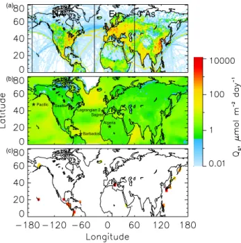
NA Eu As (a) (b) (c) ** Sagres Lagrangian 2 * * Barbados Seattle * * Algeria *Pacific

Fig. 2. Sulfur emissions for the simulation period: (a)

anthro-pogenic sources, (b) average biogenic sources, (c) average volcanic sources. All panels use the scale shown. Volcanic emissions were divided by the area of the model grid cell where the volcano is lo-cated and the surrounding grid cells have been given the same color key to increase the visibility of the location of each volcano. The north-south lines in (a) delimit the anthropogenic source regions distinguished in the model, North America (NA), Europe (Eu), Asia (As). Locations marked in panel (b) are those at which detailed source attribution was conducted for sulfate and SO2(Sect. 4).

rates of 29 to 102% day−1, SO2dry deposition rates of 3 to

32% day−1, sulfate residence times of 4 to 9 days. These dif-ferences were attributed to difdif-ferences in the relative mixing ratios of SO2and H2O2and to the fraction of SO2and sulfate

in clouds for the various source regions and source types.

2 Attribution of sulfate and SO2burdens

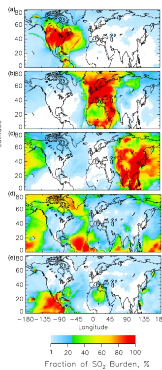
The geographic extent of the influence of individual source regions and source types is first examined using the aver-age fractional contribution to the total sulfate column burden (Fig. 3) and to the total SO2column burden (Fig. 4) for the

entire simulation period; the column burden, the vertical in-tegral of the concentration, is the pertinent quantity affecting aerosol light scattering and extinction. The average fractional contribution Frof material emitted in source region r at a

lo-cation of interest for a time period extending over multiple model time periods is calculated as:

Fr = P tBr,t P tBtot,t (1) where Br,tis the column burden at that location derived from

(a)

(b)

(c)

(d)

(e)

Fig. 3. Average fraction (%) of the different source regions and

source types to the sulfate column burden for the 6-week analysis period as a function of location in the model domain. (a) North American sources, (b) European sources, (c) Asian sources, (d) biogenic sources, and (e) volcanic sources. White indicates areas where contribution was less than 1%.

is the total column burden at that location at model time period t; fractional contribution of a source region to mix-ing ratio is evaluated similarly. As expected, each of the three major anthropogenic source regions (North America,

(a)

(b)

(c)

(d)

(e)

Fig. 4. Average fractional contribution (%) of source regions and

source types to the total SO2column burden for the 6-week

anal-ysis period, (a) North American sources, (b) European sources,

(c) Asian sources, (d) biogenic sources, and (e) volcanic sources.

White indicates areas where contribution was less than 1%.

NA; Europe, Eu; and Asia, As) was the principal contrib-utor to the column burdens in its own region, reflective of the relatively short turnover time (∼7 days) for sulfate and the much shorter turnover time (∼1 day) for SO2(Benkovitz

et al., 2004) as compared to the time needed for material to become distributed over the entire Northern Hemisphere.

a) b) c) d) e) f)

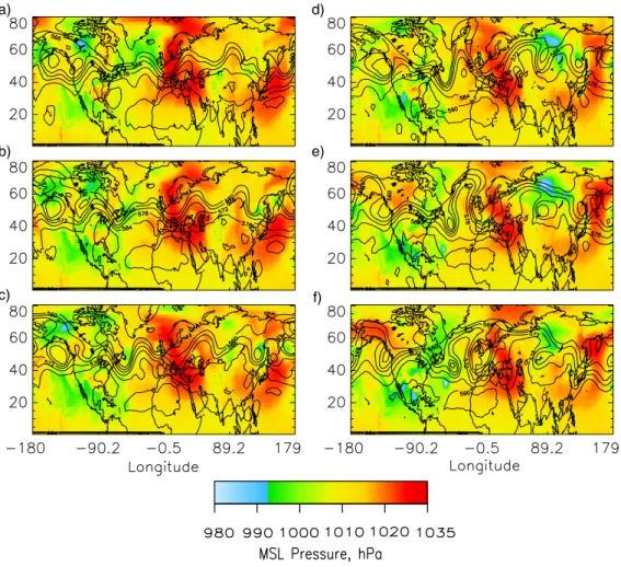
Figure 5. Mean sea level pressure (MSL, hPa) at 12UT for a) June 23, 1997, b) June 24, c) June 25, d) June 26, e) June 27, and f) June 28. Contours depict the height of the 500 hPa surface in decameters.

Fig. 5. Mean sea level pressure (MSL, hPa) at 12:00 UT for (a) 23 June 1997, (b) 24 June, (c) 25 June, (d) 26 June, (e) 27 June, and (f) 28

June. Contours depict the height of the 500 hPa surface in decameters.

In addition, the influence of each source region is extended by the transport winds and other meteorological conditions (for example, clouds responsible for aqueous conversion of SO2to sulfate) experienced during the simulation time

pe-riod. For sulfate, the large (>50%) fractional contribution from NA sources was located in a geographically concen-trated area (Fig. 3a), whereas large fractional contributions from Eu and As sources extended over much greater areas (Figs. 3b–c). It is especially notable that the large influ-ence of As sources extended over the north Pacific to Alaska, western and northern Canada, and the west coast of the U.S. (Fig. 3c). The fractional contribution from biogenic (Bio) sources was small (between 10 and 20%) except for very lim-ited areas with small sulfate burden and small contributions from other sources (Fig. 3d). The areas of large fractional contribution from volcanic (Vol) sources were southwest of Popocat´epetl volcano and west of Kilauea volcano, Hawaii (Fig. 3e). Although SO2emissions from Etna volcano were

∼40% of those from Popocat´epetl, the fractional contribu-tion of sulfate from Etna is limited to ∼25% by the large contribution to sulfate column burden from Eu sources.

Sulfate distributions were relatively delocalized from source areas because it is a secondary species with a mod-erately long turnover time. In contrast, SO2was much more

localized over source areas (Fig. 4) because it is a primary emitted species with a very short turnover time. As with sulfate, the areas of large (>50%) fractional contribution from NA sources to the SO2 burden (Fig. 4a) were more

limited than those of Eu and As sources (Figs. 4b–c). The areas of large fractional contribution from As sources ex-tended into the eastern Pacific Ocean (Fig. 4c), but the value of the average SO2 burden in this region was very small

(∼3 µmol m−2_{). Large fractional contributions from Bio}

sources were found in areas not influenced by large anthro-pogenic sources where the burdens were small, and in ar-eas of large biogenic productivity (Fig. 4d). The arar-eas of large fractional contribution from Vol sources were directly downwind of the more active volcanos, such as Popocat´epetl (Mexico), Kilauea (Hawaii), Etna (Italy), and volcanos in Japan, Indonesia, and the Kamchatka peninsula (Fig. 4e). The “contrail”-like features over the oceans, such as the one extending from northeast to southwest across the middle of

(a) (d) (b) (e) (c) (f)

Fig. 6. Modeled sulfate column burdens for 29 June 1997 12:00 UT

from (a) anthropogenic sources in North America, (b) anthro-pogenic sources in Europe, (c) anthroanthro-pogenic sources in Asia,

(d) biogenic sources, (e) volcanic sources, and (f) all sources.

White denotes areas where the sulfate column burden was less that 1 µmol m−2.

the Atlantic Ocean (especially noticeable in Fig. 4a), are due to emissions from air and ship traffic in these corridors (Fig. 2a). These features are not evident in the sulfate distri-butions.

3 Meteorological influences

Here the influence of transport meteorology on the fractional contribution to the column burdens from emissions in the several source regions is examined via the mean sea level pressure, MSL, for 23 June to 28 June 1997 (Fig. 5); con-ditions on these days were representative of the entire sim-ulation period. On 29 June column burdens of SO2 and

sulfate (Fig. 6) were affected by four major features of the global sea level pressure: large high pressure systems off the coast of Japan and over Europe, a low pressure system over northern Mexico and the eastern Pacific Ocean, and a strong low pressure system over Siberia. Transport of Asian emissions from sources located between 20◦N and 40◦N (Fig. 2a) to the north along the eastern coast of Asia and then eastward over the northern Pacific Ocean is evident in Fig. 6c. This transport was driven by clockwise flow around the high pressure system off the coast of Japan from 23 June to 25 June (Figs. 5a–c). After 25 June this high pressure system migrated northward, and a low pressure system de-veloped in conjunction with an upper level cutoff low over Siberia and Eastern Asia (Fig. 5d). The low pressure system further enhanced northward transport of sulfate from emis-sions in southeast Asia; this was followed by flow around the high pressure system, which then transported the sul-fate eastward across the Pacific at higher latitudes. From 23 June through 27 June (Figs. 5a–e) a large high pressure system over western Europe generated light winds and lit-tle vertical mixing, preventing transport of European emis-sions and enhancing production of sulfate. On 25 and 26 June (Figs. 5c–d) there was a decrease in surface pressure in phase with a deepening ridge-trough system at upper lev-els over Spain and north of the Indian sub-continent; coun-terclockwise flow around these systems transported sulfate from European sources northward (by the system over Spain) to Scandinavia and southward (by the system over India) to the Middle East. The low pressure that formed over Siberia on 25 June (Fig. 5c) enabled the eastward transport of sulfate from European sources to western and central Asia.

For several days preceding 28 June the North American continent was dominated by a deepening low pressure system over the southwestern U.S. and northern Mexico consistent with divergence at the 500 hPa level (Figs. 5a–e). A surface high pressure system was located over the southeastern U.S. through 27 June; on 28 June (Fig. 5f) there were low pressure systems over the Midwest U.S. and over the Gulf of Mexico. Counterclockwise flow associated with these systems trans-ported emissions from the major east coast sources over the Atlantic Ocean (Fig. 6a). A deepening trough and associated

surface low pressure center in the Atlantic Ocean (Fig. 5f) kept the maximum sulfate column burden south of 35◦_N

until the eastern side of the pressure center (∼45◦_{W) was}

reached, when emissions were transported towards the north Atlantic. These meteorological patterns assist in explaining features seen in the average fractional contribution to the sul-fate and SO2burden (Figs. 3 and 4) such as the abrupt

de-crease in the contribution of NA sources at the west coast of the continent, the large influence of As sources over the western and northern Pacific Ocean, and of Eu sources over the Middle East, extending to central Asia and the Atlantic Ocean south of 20◦N and north of 60◦N for sulfate.

In the interactive discussion of this paper one of the anony-mous reviewers suggested that links between meteorology and concentration or burden might be strengthened, perhaps by the use of trajectory analysis. As noted in the introduc-tion several investigators have in fact used trajectory calcula-tions to attribute modeled species to source regions, at least qualitatively. Here, rather than using trajectory analysis we have taken the approach of attributing sulfate (and SO2) to

large source regions by labeling the sulfur species according to several source regions. We take this approach for several reasons: First, the labeling approach readily yields quanti-tative estimates of contributions to concentration from the several source regions; second, as the source regions con-sidered here are continental in scale, they are not well suited to examination by trajectory analysis; third, the accuracy of trajectories decreases markedly after ∼5 days; fourth, the use of different assumptions and methodologies in trajec-tory calculations can yield quite different results; and finally, trajectory-based approaches cannot accurately represent non-linear chemical reactions, such as the H2O2-SO2 reaction,

which is dominant in sulfate formation. As an alternative means of relating atmospheric burdens of sulfate and SO2

to emissions regions, we would invite the reader to exam-ine the animations of the column burdens of these substances taken from the model output at 6-h intervals, available at http://www.ecd.bnl.gov/steve/model/junejuly97.html, which are an effective way to follow the transport of these sub-stances.

4 Attribution by source regions

Three locations in areas in which there were substantial con-tributions to sulfate mixing ratios and burdens from two or more source regions or source types (Fig. 2b) were selected to illustrate the temporal variability and the vertical structure of these contributions: the model grid cells that include Seat-tle, WA, USA (122.20◦W, 47.36◦N, grid cell surface height 0.1 km), Sagres, Portugal (8.95◦W, 36.98◦N, grid cell sur-face height <0.01 km), and Barbados (59.43◦W, 13.17◦N, grid cell surface height <0.01 km). Time series of the sul-fate column burden for these three locations (Figs. 7a–c) ex-hibit substantial variation in the absolute and relative

con-(a)a)

(b)b)

(c)c)

(d)d)

Fig. 7. Time series of the sulfate column burden attributable to the

different source regions and source types in magnitude (left) and as fraction of total (right) at several locations shown in Fig. 2. (a) model grid cell that includes Seattle, WA, USA (122◦W, 47◦N),

(b) model grid cell that includes Sagres, Portugal (8◦W, 36◦N), and

(c) model grid cell that includes Barbados (59◦W, 13◦N). Panel (d)

shows similar time series for the SO2column burden at a model grid

cell in the mid north Pacific Ocean (170◦W, 47◦N).

tributions from the different source regions. At Seattle the apportionment of the column burden for the entire model-ing period was As sources 42%, NA sources 32%, and Eu sources 16%. Despite the long transit across the north Pa-cific As sources were the principal contributors on two of the three instances of largest magnitude of the total col-umn burden (Fig. 7a). At Sagres the apportionment was Eu sources 52%, NA sources 26%, and As sources 13%. The situation at Barbados (Fig. 7c) was much more com-plicated; the apportionment here was Bio sources 27%, Eu sources 26%, NA sources 17%, and Vol sources 17%. At different time periods each of the different source regions and source types (except As sources) was the major contrib-utor to the column burden. Sulfate from NA sources reach-ing Barbados was transported east across the North Atlantic, south along the west coasts of Europe and Africa and west to Barbados via the trade winds at lower latitudes. Sulfate from Eu sources reaching Barbados was transported south

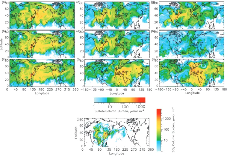
(a) (b) (c) (d) (e) (f) (g) (h) (i) (j) k)

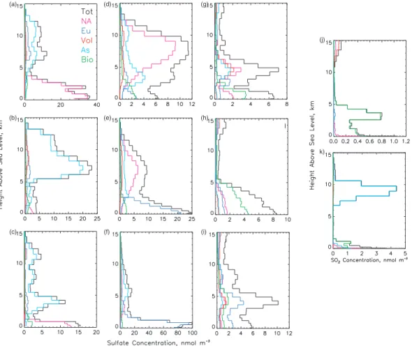
Fig. 8. Vertical profiles of the sulfate concentration attributable to the different source regions and source types at several locations shown in

Fig. 7. Model grid cell that includes Seattle, WA, USA (122◦W, 47◦N) on (a) 4 July 1997 12:00 UT, (b) 7 July 00:00 UT, and (c) 7 July 12:00 UT; model grid cell that includes Sagres, Portugal (8◦W, 36◦N) on (d) 4 July 18:00 UT, (e) 5 July 12:00 UT, and (f) 9 July 18:00 UT; model grid cell that includes Barbados (59◦W, 13◦N) on (g) 7 July 12:00 UT, (h) 9 July 06:00 UT, and (i) 23 July 12:00 UT. Vertical profiles of the SO2concentration attributable to the different source regions and source types at (j) Barbados on 9 July 06:00 UT, and (k) a model

grid cell in the mid north Pacific Ocean (170◦W, 47◦N) on 17 July 06:00 UT. Note the individual scale for the concentration axis on each panel.

along western Europe and Africa and west to Barbados via the trade winds. Sulfate from As sources reaching Barba-dos was transported east across the North Pacific, across North America, and then followed the same path as sulfate from NA sources. Animations of the sulfate and SO2

col-umn burdens from each source region are available at URL http://www.ecd.bnl.gov/steve/model/junejuly97.html.

Vertical profiles of the sulfate concentration for these lo-cations at selected times (Fig. 8) show marked differences in the distribution with height of the contribution attributable to the different source regions and types. At Seattle on 4 July 1997 (Fig. 8a) the maximum concentration was near the sur-face and NA sources dominated below 3 km; above 6 km the principal contributors were As sources, with a smaller but perceptible contribution from Eu sources. Sulfate from Eu sources reaching Seattle is transported east across Europe, Asia, and the North Pacific Ocean. A very different picture is presented on 7 July, at 00:00 UT. On this date the largest

concentration was substantially displaced from the surface (∼7 km) and quite isolated from low altitude processes; the principal contributors above 5 km were As sources; below this height several source regions and source types con-tributed almost equally to a much smaller concentration. Just 12 h later (Fig. 8c) the picture was again quite different, with considerably lower concentrations overall. The maximum concentration was in a shallow layer below 1 km, contributed mostly by NA sources, but there was still substantial mate-rial from As sources aloft, and these sources continued to dominate the column burden. The influence of As sources at Seattle for these three dates is demonstrated using the sulfate column burden (Figs. 9a–c). On 4 July at 12:00 UT the Asian plume entered the Seattle area from the southwest (Fig. 9a); the full effect of this plume was felt on 7 July at 00:00 UT (Fig. 9b), and by 7 July at 12:00 UT the plume had passed to the east of Seattle (Fig. 9c).

   St St St  Sa Sa   Ba Ba Ba (a) (b) (c) (d) (e) (f) (g) (h) (i) Sa (j) _P

Fig. 9. Sulfate column burden from (a) Asian sources on 4 July 1997 12:00 UT, (b) Asian sources on 7 July 00:00 UT, (c) Asian sources

on 7 July 12:00 UT, (d) North American sources on 4 July 18:00 UT, (e) North American sources on 5 July 12:00 UT, (f) European sources on 9 July 18:00 UT, (g) North American sources on 7 July 12:00 UT, (h) biogenic sources on 9 July 06:00 UT, and (i) European sources on 23 July 12:00 UT. SO2column burden from (j) Asian sources on 17 July 06:00 UT. St= Seattle, Sa= Sagres, Ba= Barbados, P= mid north

Pacific Ocean location. White denotes areas where the column burden from individual source was less that 1 µmol m−2.

At Sagres the maximum sulfate concentrations varied by almost a factor of eight (∼13 to 100 nmol m−3)for the dates presented here. On 4 July 1997 at 18:00 UT (Fig. 8d) the concentration was small; NA sources were the principal con-tributors in a fairly deep layer between 6 and 8 km where the largest concentration (∼13 nmol m−3)was located. On 5 July at 12:00 UT (Fig. 8e) the principal contributors be-low 2.5 km were Eu sources and the largest concentration was at the surface (∼25 nmol m−3_{); in addition there was a}

plume between 3 and 12 km where the principal contributors were NA sources. On 9 July at 18:00 UT (Fig. 8f) the princi-pal contributors below 3 km were Eu sources and the largest concentration was also at the surface (∼100 nmol m−3); the principal contributors above 4 km were As sources, and the concentration (∼15 nmol m−3)was similar to that on 4 July at 18:00 UT. The animation of the sulfate column burden from As sources showed that the contribution from these sources was transported in a wave pattern across the Pacific

Ocean at ∼40◦N latitude, across North America at ∼45◦N, across the Atlantic Ocean at ∼50◦N and finally southward over Sagres. The influence of NA and Eu sources on Sagres is shown in Figs. 9d–e. On 4 July 1997 at 18:00 UT (Fig. 9d) the plume from NA sources had reached Sagres from the west via a wave pattern across the Atlantic Ocean (see anima-tion). By 5 July at 12:00 UT the column burden from these sources had started to decrease (Fig. 9e), and on 9 July at 18:00 UT (Fig. 9f) the large column burden from Eu sources had advanced over Sagres from the east (see animation).

Barbados presented a more complicated picture because several source regions and source types were the main con-tributors or contributed about equally to the sulfate concen-tration at different times. On the three dates shown the sul-fate concentration was similar (∼10 nmol m−3)but up to a factor of five to ten less than at Seattle and Sagres, mainly a consequence of this location being well removed from major emission sources. An example of a very mixed picture is that

for 7 July (Fig. 8g). On this date sulfate was present mostly in two distinct layers, one below 2 km to which Bio sources contributed slightly over half and to which NA sources con-tributed ∼30% of the concentration, and a second layer, be-tween 4 and 6 km, to which NA, Vol, and As sources con-tributed almost equally. On 9 July (Fig. 8h) most of the mate-rial was in a deep layer extending from the surface to ∼6 km, to which Bio sources from the Atlantic ocean south of 25◦N (Fig. 2b) were the largest contributors below 6 km; how-ever, about half of the concentration in this altitude range was contributed by other source regions and types. On 23 July at 12:00 UT (Fig. 8i) three somewhat distinct layers were evident; from the surface to ∼2 km and also from 2 km to 4 km Eu sources contributed ∼40% of the concentration, with all other source regions and source types contributing about equally to the remaining 60%. All source types con-tributed about equally to the third layer, centered at ∼8 km. The influence of NA, Bio, and Eu sources on Barbados is seen also in the sulfate column burden (Figs. 9g–i).

In contrast to the distribution of sulfate, time series of the SO2column burden at the selected locations showed that the

major contributors were always proximate sources: North American sources at Seattle (∼96%), European sources at Sagres (∼94%), and biogenic sources at Barbados (∼64%). However, at Barbados some vertical structure was apparent during certain time periods, for example on 9 July 06:00 UT (Fig. 8j) Bio and NA sources contributed almost equally at the surface, but the NA contribution dropped rapidly with height whereas at the altitude of the maximum total concen-tration, ∼3 km, the SO2was contributed by Bio sources.

The influence of Asian sources on the SO2 burden over

the mid north Pacific Ocean was examined at 170◦_W,

47◦_{N (Fig. 2b). At this location (∼4300 km from Tokyo;} ∼5700 km from Beijing, major source regions on the Asian continent) As sources were responsible for more than half of the SO2 burden for the entire simulation period. Time

series of the SO2 column burden at this location (Fig. 7d)

showed that As sources were frequently the dominant con-tributors. The distribution of the SO2 column burden from

these sources during one of the time periods of large influ-ence (17 July 06:00 UT, Fig. 9j) showed a narrow plume that meandered across the north Pacific Ocean. The vertical profile of the SO2 concentration (Fig. 8k) at the mid ocean

location showed that almost all the SO2from these sources

was quite elevated, in a layer at altitudes of between ∼7 and 11 km. At such altitudes SO2is immune to removal by one of

its major sinks, dry deposition and can thus persist for con-siderable time. Compact aerosol layers have been observed to travel great distances in the upper troposphere (Damoah et al., 2004; Jaffe et al., 2004; Ansmann et al., 2002; Wandinger et al., 2002; Forster et al., 2001).

Because of the short time period examined in the present study it is not known how representative the instances cho-sen for detailed examination, Seattle, Sagres, and Barbados are of the northwestern North American coastal region, the

coastal European, and the trade winds of the North Atlantic, respectively. Clearly the temporal variability of the control-ling meteorology plays a large role in the absolute and rel-ative contributions of distant and proximate sources to the sulfate burden at a given location and time. Nonetheless the cases examined here show that distant sources can make a substantial contribution to the column burden of sulfate at the locations under examination.

5 Attribution of sulfate burden by formation process

Sulfur dioxide is converted to sulfate in the model by two dif-ferent processes: gas-phase oxidation by OH in clear (cloud-free) air and aqueous-phase oxidation by H2O2 and O3 in

cloud water. As the model associates the sulfate formed by different processes with different sulfate variables, it is pos-sible to examine the amount of sulfate present at a given time and location that has been formed by one or the other process. For the entire simulation period ∼62% of the sulfate present in the model domain was formed by aqueous-phase oxida-tion and ∼36% by gas-phase oxidaoxida-tion; ∼2% was primary sulfate. However the fractional contributions by the two oxi-dation mechanisms varied considerably as a function of loca-tion and, at a given localoca-tion, as a funcloca-tion of time during the model run. For example, more than half the sulfate present in geographic regions with sparse cloudiness and precipitation, such as North Africa and the Middle East, and in regions with sources at high altitude, such as Mexico, was formed by gas-phase oxidation. The spatial and temporal variation in formation mechanism is due mainly to differences in me-teorological conditions, most importantly the presence and liquid water content of clouds. While it must be recognized that the sulfate present at a specific time and location is a mix of material formed locally and material transported to that lo-cation, nonetheless examination of formation mechanism of the sulfate present at specific locations and times allows in-ferences to be drawn about the reasons for the difin-ferences.

Two contrasting locations (Fig. 2b) were chosen to study the time variation of the sulfate formation processes. At a semi-desert area of Algeria (5◦E, 22◦N, grid cell surface height 1.1 km) ∼58% of the sulfate present over the entire simulation period was formed via gas-phase oxidation, and gas-phase oxidation was the principal contributor to the bur-den at this location at all times during the model period ex-cept for a few days around 30 June, Fig. 10a. The animation of the SO2burden reveals that periods of larger contribution

from gas-phase oxidation occurred when large amounts of SO2from the European continent were transported over the

arid areas of North Africa, with the oxidation taking place over the Sahara region of Africa where the prevailing mete-orological conditions (strong solar radiation, abundant OH, and low cloud water content) favor conversion to sulfate via this mechanism. On days with little transport of SO2from

Gas Gas Aq Aq Prim Prim (a) (b)

Fig. 10. Time series of the sulfate burden at (a) Algeria (5◦E, 22◦N), and (b) a location in the North Atlantic off the coast of Portugal

(12◦W, 39◦N).

North African location was formed en route (over the Euro-pean continent and the Mediterranean Sea), where conditions favored formation via aqueous-phase oxidation.

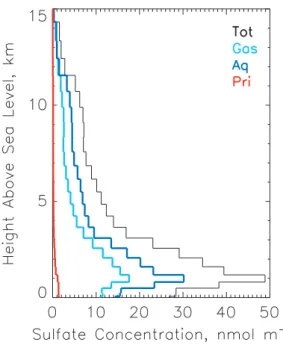
A contrasting situation is found over the western North At-lantic Ocean (Fig. 2b). Here, in order to permit comparison with measurements, we examined the model results in the study area of the ACE-2 cloudy Lagrangian-2 experiments, which were conducted 16 July to 18 July off the west coast of Portugal and Africa (11◦to 15◦W, 32◦to 40◦N, surface height 0) (Johnson et al., 2000a, b). At this location the dom-inant formation mechanism throughout the entire simulation period was aqueous-phase oxidation (Fig. 10b). The main features of the modeled vertical profile of the sulfate con-centration (Fig. 11) at the approximate time and location of aircraft measurements during this study are consistent with the measured profiles of accumulation mode aerosol concen-tration reported in Fig. 7 of Johnson et al. and with the mea-sured concentration of total condensation nuclei in Fig. 7 of Osborne et al. (2000) which show these quantities exhibiting a maximum below 1 km and decreasing with increasing alti-tude above. In addition, the larger contribution below 3 km of sulfate formed by aqueous-phase conversion supports the conclusions of Dore et al. (2000) that increases in the total aerosol mass at these altitudes observed during their experi-ment represented the net contribution to aerosol via conver-sion from gaseous precursors and that this converconver-sion most probably occurred via in-cloud aqueous-phase reaction.

Summarizing Sects. 4 and 5, the time series of the sul-fate column burden by source region and source type at spe-cific locations for the entire simulation period and vertical profiles of the sulfate concentration for specific times and locations demonstrate the large temporal variability, the fre-quently large fractional contribution by remote sources, and

Fig. 11. Vertical profile of the sulfate concentration at 12◦W, 39◦N

on 16 July 1997 at 00:00 UT.

the frequent occurrence of maximum concentrations well aloft. Not infrequently, important contributions to the con-centration from remote sources were located in elevated lay-ers; thus these source regions contribute more to column properties such as optical depth than to surface air quality. At Barbados, well removed from major sources and influ-enced by several source regions and source types, even sur-face concentrations were substantially impacted by remote sources. The relative contributions of the gas-phase and the

aqueous-phase oxidation pathways to the sulfate column bur-den at particular locations were influenced by meteorological conditions encountered during transport.

The most important factors affecting the distribution of both sulfate and SO2were the locations of emissions sources

and predominant meteorological conditions. Because of its longer turnover time of ∼7 days (Benkovitz et al., 2004), sulfate was transported further from the source regions than was SO2 (turnover time ∼1 day), with conversion taking

place concurrent with transport. Emitted species were gener-ally transported from west to east, but substantial northward transport was identified for emissions from Asian sources and additional northward and southward transport was iden-tified for emissions from European sources. In addition, in-tercontinental transport of aerosols, already identified in spe-cific instances by measurements (Jaffe et al., 2003; Perry et al., 1999; Prospero, 1999; Wotawa and Trainer, 2000) and satellite observations (Husar et al., 2001), has been illustrated in the present modeling results.

6 Summary and implications

Results from an Eulerian chemical transport model have been analyzed to attribute sulfate and SO2concentrations and

col-umn burdens to specific source regions, source types and sulfate formation processes. Because of the relatively short turnover times of these species proximate anthropogenic sources were the principal contributors to the burdens in the several regions, but the influence of North American sources was dominant over almost all of the North Atlantic Ocean, and likewise the influence of Asian sources was dominant over almost all of the North Pacific Ocean. At a given lo-cation not infrequently distant source regions contributed widely differing fractional amounts of sulfate, especially when the peak of the vertical distribution of concentration was highly elevated. At Seattle, WA, U.S. Asian sources contributed 42% and European sources contributed 16% of the column burden for the simulation period as a whole; the largest contribution from Asian and European sources oc-curred in layers above ∼3 km. At Sagres, Portugal, North American sources contributed 26% and Asian sources con-tributed 13% of the column burden; when the total column burden was small North American sources were the largest contributor, mainly in layers 5 km above the surface. Smaller contributions from Asian sources were occasionally seen as layers at altitudes above ∼4 km; these layers had been trans-ported eastward across the Pacific Ocean, North America, and the Atlantic Ocean.

Overall, the average contribution to the sulfate burden for the entire simulation period was 62% from aqueous-phase oxidation, 36% from gas-phase oxidation and 2% was pri-mary sulfate; however, in areas of low cloudiness, such as north Africa and the Middle East, or areas at high altitudes, such as parts of Mexico, the fraction of sulfate formed by

gas-phase oxidation was considerably enhanced, over 50%. At locations of low cloudiness where gas-phase oxidation was the main contributor to the sulfate concentration for cer-tain time periods aqueous-phase oxidation was the main con-tributor in layers above the surface, as a consequence of long-range transport from cloudy areas.

It should be emphasized that the objective of the present study was to examine the extent to which distant sources contribute to the absolute and relative column burden of sul-fate at specific locations at specific times, and the variabil-ity of these contributions during the time period examined, rather than to develop a statistically or climatologically ro-bust attribution. Here we relied on a set of model runs that had been rigorously evaluated by comparison with observa-tions at specific locaobserva-tions and for short time periods, typi-cally, for sulfate, 24 h, but was, perforce, limited to a rather short model run, six weeks of a single year. While this rather short time period necessarily limits any generalization of the findings, the present findings nonetheless demonstrate instances in which the sulfate column burden at a given loca-tion was dominated by material that was transported across major oceanic basins and also demonstrate the high temporal variability of the relative and absolute contributions of this distant sulfate to the column burden at a given location.

In summary the present study contributes to a growing body of evidence indicative of the importance of long range transport of submicrometer aerosols on scales of several thousand kilometers. This contribution is especially impor-tant in a relative sense in regions of low background aerosol, such as over the North Pacific and North Atlantic where it might be expected to contribute strongly to aerosol in-direct forcing in view of the low natural aerosol loading, which leads to high sensitivity to incremental aerosol loading (Schwartz et al., 2002). Such loadings can also be substan-tial in an absolute sense. For example in the calculations presented here for Seattle, the contribution of Asian sources to sulfate column burden was commonly 20 µmol m−2 and occasionally greater than 100 µmol m−2(2–10 mg m−2); for a mass scattering efficiency of 5–8 m2g−1(Charlson et al., 1992) this burden would result in an optical depth of 0.01 to 0.08. In turn, for an aerosol radiative forcing efficiency of −40 to −50 W m−2 per optical depth (24-h; top of at-mosphere; Anderson et al., 2005) this aerosol optical depth would result in a direct radiative forcing of 0.4 to 4 W m−2. In contrast, because the long-range-transported aerosol was generally well elevated above the surface, it would appear that this aerosol makes a relatively small contribution to sur-face concentrations pertinent to air quality considerations.

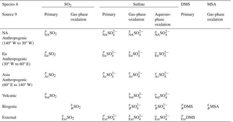
Table A1. Schematic of the different species defined as variables in the model. Superscripts: a=aqueous-phase oxidation, g=gas-phase

oxidation, p=primary emission. Subscripts: As=Asia, B=biogenic, Eu=European, Ext=external (coming from outside the model domain), NA=North American, Vol=volcanic.

Species 6 SO₂ Sulfate DMS MSA

Source 9 Primary Gas-phase

oxidation Primary Gas-phase oxidation Aqueous-phase oxidation Primary Gas-phase oxidation NA Anthropogenic (140◦W to 30◦W) p NASO2 pNASO 2− 4 g NASO 2− 4 a NASO 2− 4 Eu Anthropogenic (30◦W to 60◦E) p EuSO2 pEuSO 2− 4 g EuSO 2− 4 aEuSO 2− 4 Asia Anthropogenic (60◦E to 140◦W) p AsSO2 pAsSO 2− 4 g AsSO 2− 4 aAsSO 2− 4

Volcanic p_VolSO2 gVolSO

2−

4 aVolSO 2− 4

Biogenic g_BSO2 g_BSO2−₄ a_BSO2−₄ p_BDMS g_BMSA

External g_ExtSO₂ p_ExtSO2−_{4 Ext}g SO2−₄ a_ExtSO2−₄ p_ExtDMS

Appendix A

Description of the Eulerian model

The Eulerian model used in this work was developed from the model described in (Benkovitz et al., 1994). The model represents emissions of sulfur dioxide (SO2)and dimethyl

sulfide (DMS), transport, convective mixing, generation of hydrogen peroxide (H2O2) from the hydroperoxy radical

(HO2)in the gas-phase, chemical conversion of SO2to

sul-fate by H2O2and ozone (O3)in the aqueous-phase and by

the hydroxyl radical (OH) in the gas-phase, chemical con-version of DMS to SO2and MSA by OH, wet removal, and

dry deposition (Fig. 1). A hemispheric domain was used in this study because it incorporates all industrialized areas of the Northern Hemisphere, allows studies of the relative in-fluences of the various source regions and source types and minimizes import/export of material into/out of the model domain. Because the chemistry of sulfur species alters atmo-spheric concentrations of oxidant species, the influence of source regions and source types was obtained by defining a different variable for each source region/type (Table A1) and performing only a single simulation; this method provides accurate estimates of such influences. The model was initial-ized with the mixing ratio of all species set to zero; material transported into the model domain was assigned representa-tive background concentrations and was carried as a separate variable.

The meteorological data used to drive the model, for the modeling period 1 June–31 July 1997, were obtained from the European Centre for Medium-Range Weather Forecasts (ECMWF) (European Centre for Medium-Range Weather Forecasts, 2003). Mixing ratios (MRs) of oxidant species were based on monthly average MRs for June and July cal-culated using Version 2 of the Model of Ozone and Re-lated Chemical Tracers, (MOZART) (Brasseur et al., 1998; Horowitz et al., 2003) driven by a GCM, the NCAR Commu-nity Climate Model. Anthropogenic emissions of SO2were

based on the Emission Database for Global Atmospheric Re-search (EDGAR) Version 3.2 (Olivier et al., 2002) inven-tory, which represents annual emissions ca. year 1995. Sea-sonal emissions and the breakdown between release points below and above 100 m were calculated using the appro-priate fractions from the Global Emissions Inventory Activ-ity (GEIA) Version 1B inventory (Benkovitz et al., 1996); emissions for the Northern Hemisphere summer were used. Emissions of primary sulfate for 1997 were estimated from the GEIA SO2inventory as 1% of the sulfur emissions (by

mole) for industrialized regions (North America, Europe) and 2% for the rest of the model domain. Sea surface DMS concentrations for June and July from Kettle et al. (1999) were combined with seawater DMS measurements made during the Aerosol Characterization Experiment-2 (ACE-2) field campaign (Raes and Bates, 1995) to calculate time-and location-dependent oceanic DMS emissions using the

wind speed transfer velocity relationship of Liss and Mer-livat (1986). Seasonal emissions of DMS and hydrogen sulfide (H2S) from land sources were calculated using the

methodology of Lamb (Bates et al., 1992) gridded to 1◦×1◦ resolution (Benkovitz et al., 1994); these emissions were treated entirely as DMS in the model. Volcanic emissions are quite variable temporally and there were substantial volcanic events during the modeling period, so as far as possible daily sulfur emissions from volcanos were specific to the simula-tion period and were treated entirely as SO2. The principal

sources of time-specific information were the Volcano Ac-tivity Reports compiled by the Global Volcanism Program of the Smithsonian Institution available at web site http://www. volcano.si.edu/reports/bulletin/index.cfm (accessed in spring 1999) and personal communications from investigators con-ducting measurements at individual volcanos.

Acknowledgements. Research was performed under the auspices

of the U.S. Department of Energy under Contract No. DE-AC02-98CH10886 and was supported in part by the NOAA Office of Global Programs. The meteorological data used to drive the model were obtained from the European Centre for Medium-Range Weather Forecasts (ECMWF), Reading, UK.

Edited by: F. J. Dentener

References

Allan, J. D., Bower, K. N., Coe, H., Boudries, H., Jayne, J. T., Canagaratna, M. R., Millet, D. B., Goldstein, A. H., Quinn, P. K., Weber, R. J., and Worsnop, D. R.: Submicron aerosol com-position at Trinidad Head, California, during ITCT 2K2: Its re-lationship with gas phase volatile organic carbon and assessment of instrument performance, J. Geophys. Res.-Atmos., 109(D23), D23S24, doi:10.1029/2003JD004208, 2004.

Anderson, T. L., Charlson, R. J., Bellouin, N., Boucher, O., Chin, M., Christopher, S. A., Haywood, J., Kaufman, Y. J., Kinne, S., Ogren, J. A., Remer, L. A., Takemura, T., Tanr´e, D., Tor-res, O., Trepte, C. R., Wielicki, B. A., Winker, D. M., and Yu, H.: A-Train strategy for quantifying direct climate forcing by an-thropogenic aerosols, Bull. Am. Meteorol. Soc., 86, 1795–1809, 2005.

Ansmann, A., Wandinger, U., Wiedensohler, A., and Leiterer, U.: Lindenberg Aerosol Characterization Experiment 1998 (LACE 98): Overview, J. Geophys. Res., 107(D21), 8129, doi:10.1029/2000JD000233, 2002.

Bates, T. S., Lamb, B. K., Guenther, A., Dignon, J., and Stoiber, R. E.: Sulfur Emissions to the Atmosphere from Natural Sources, J. Atmos. Chem., 14, 315–337, 1992.

Bellouin, N., Boucher, O., Haywood, J., and Reddy, M. S.: Global estimate of aerosol direct radiative forcing from satellite mea-surements, Nature, 438, 1138–1141, doi:10.1038/nature04348, 2005.

Benkovitz, C. M., Berkowitz, C. M., Easter, R. C., Nemesure, S., Wagener, R., and Schwartz, S. E.: Sulfate Over the North At-lantic and Adjacent Continental Regions: Evaluation for Oc-tober and November, 1986 Using a Three-Dimensional Model

Driven by Observation-Derived Meteorology, J. Geophys. Res., 99(D10), 20 725–20 756, 1994.

Benkovitz, C. M., Scholtz, M. T., Pacyna, J., Tarras´on, L., Dignon, J., Voldner, E. V., Spiro, P. A., Logan, J. A., and Graedel, T. E.: Global Gridded Inventories of Anthropogenic Emissions of Sul-fur and Nitrogen, J. Geophys. Res., 101(D22), 29 239–29 253, 1996.

Benkovitz, C. M., Schwartz, S. E., and Kim, B.-G.: Evaluation of a Chemical Transport Model for Sulfate using ACE-2 Ob-servations and Attribution of Sulfate Mixing Ratios to Source Regions and Formation Processes, Geophys. Res. Lett., 30(12), doi:10.1029/2003GL016942, 2003.

Benkovitz, C. M., Schwartz, S. E., Jensen, M. P., Miller, M. A., Easter, R. C., and Bates, T. S.: Modeling atmospheric sulfur over the Northern Hemisphere during the Aerosol Characteriza-tion Experiment 2 experimental period, J. Geophys. Res., 109, D22207, doi:10.1029/2004JD004939, 2004.

Bott, A.: A Positive Definite Advection Scheme Obtained by Non-linear Renormalization of the Advective Fluxes, Mon. Wea. Rev., 117, 1006–1015, 1989.

Brasseur, G., Hauglustaine, D., Walters, S., Rasch, P., M¨uller, J., Granier, G., and Tie, X. X.: MOZART: A Global Chemical Transport Model for Ozone and Related Chemical Tracers. 1. Model Description, J. Geophys. Res., 103(D21), 28 265–28 289, 1998.

Charlson, R. J., Schwartz, S. E., Hales, J. M., Cess, R. D., Coakley Jr., J. A., Hansen, J. E., and Hofmann, D. J.: Climate forcing by anthropogenic aerosols, Science, 255, 423–430, 1992.

Damoah, R., Spichtinger, N., Forster, C., James, P., Mattis, I., Wandinger, U., Beirle, S., Wagner, T., and Stohl, A.: Around the World in 17 days – Hemispheric-Scale Transport of Forest Fire Smoke from Russia in May 2003, Atmos. Chem. Phys., 4, 1311–1321, 2004,

http://www.atmos-chem-phys.net/4/1311/2004/.

Dore, A. J., Johnson, D. W., Osborne, S. R., Choularton, T. W., Bower, K. N., Andreae, M. O., and Bandy, B. J.: Evolution of Boundary-Layer Aerosol Particles Due to In-Cloud Chemi-cal Reactions During the 2nd Lagrangian Experiment of ACE-2, Tellus, 52B(2), 452–462, 2000.

Easter, R. C.: Two Modified Versions of Bott’s Positive Definite Numerical Advection Scheme, Mon. Wea. Rev., 121, 297–304, 1993.

Easter, R. C. and Luecken, D. J.: A Simulation of Sulfur Wet De-position and Its Dependence on the Inflow of Sulfur Species to Storms, Atmos. Environ., 22(12), 2715–2739, 1988.

European Centre for Medium-Range Weather Forecasts: IFS Doc-umentation Cycle CY25r1 Parts I–VII, European Centre for Medium-Range Weather Forecasts, Reading, England, 2003. Forster, C., Wandinger, U., Wotawa, G., James, P., Mattis, I.,

Althausen, D., Simmonds, P., O’Doherty, S., Jennings, S. G., Kleefeld, C., Schneider, J., Trickl, T., Kreipl, S., J¨ager, H., and Stohl, A.: Transport of Boreal Forest Fire Emissions from Canada to Europe, J. Geophys. Res., 106(D19), 22 887–22 906, 2001.

Graf, H.-F., Feichter, J., and Langmann, B.: Volcanic Sulfur Emis-sions: Estimates of Source Strenght and Its Contribution to the Global Sulfate Distribution, J. Geophys. Res., 102(D9), 10 727– 10 738, 1997.

Granier, C., Tie, X., Lamarque, J. F., Schultz, M., and Brasseur, G.: A global simulation of tropospheric ozone and related trac-ers: Description and evaluation of MOZART, version 2, J. Geo-phys. Res., 108(D24), 4784, doi:10.1029/2002JD002853, 2003. Husar, R. B., Tratt, D. M., Schichtel, B. A., Falke, S. R., Li, F.,

Jaffe, D., Gass´o, S., Gill, T., Laulainen, N. S., Lu, F., Reheis, M. C., Chun, Y., Westphal, D., Holben, B. N., Gueymard, C., McKendry, I., Kuring, N., Feldman, G. C., McClain, C., Frouin, R. J., Merrill, J., DuBois, D., Vignola, F., Murayama, T., Nick-ovic, S., Wilson, W. E., Sassen, K., Sugimoto, N., and Malm, W. C.: Asian dust events of April 1998, J. Geophys. Res., 106(D16), 18 317–18 330, doi:10.1029/2000JD900788, 2001.

Jaffe, D., Anderson, T., Covert, D., Kotchenruther, R., Trost, B., Danielson, J., Simpson, W., Berntsen, T., Karlsdottir, S., Blake, D., Harris, J., Carmichael, G., and Uno, I.: Transport of Asian Air Pollution to North America, Geophys. Res. Lett., 26(6), 711– 714, 1999.

Jaffe, D., McKendry, I., Anderson, T., and Price, H.: Six ‘New’ Episodes of Trans-Pacific Transport of Air Pollutants, Atmos. Environ., 37, 391–404, 2003.

Jaffe, D., Bertschi, I., Jaegl´e, L., Novelli, P., Reid, J. S., Tanimoto, H., Vingarzan, R., and Westphal, D. L.: Long-Range Trans-port of Siberian Biomass Burning Emissions and Impact on Sur-face Ozone in Western North America, Geophys. Res. Lett., 31, L16106, doi:10.1029/2004GL020093, 2004.

Johnson, D. W., Osborne, S., Wood, R., Suhre, K., Johnson, R., Businger, S., Quinn, P. K., Wiedensohler, A., Durkee, P. A., Rus-sell, L. M., Andreae, M. O., O’Dowd, C., Noone, K. J., Bandy, B., Rudolph, J., and Rapsomanikis, S.: An Overview of the Lagrangian Experiments Undertaken During the North Atlantic Aeorosol Characterisation Experiment (ACE-2), Tellus, 52B(2), 290–320, 2000a.

Johnson, R., Businger, S., and Baerman, A.: Lagrangian Air Mass Tracking with Smart Balloons During ACE-2, Tellus, 52B(2), 321–334, 2000b.

Kettle, A. J., Andreae, M. O., Amoroux, D., Andreae, T. W., Bates, T. S., Berresheim, H., Bingemer, H., Boniforti, R., Curran, M. A. J., DiTullio, G. R., Helas, G., Jones, G. B., Keller, M. D., Kiene, R. P., Leck, C., Levasseur, M., Malin, G., Maspero, M., Matrai, P., McTaggart, A. R., Mihalopoulos, N., Nguyen, B. C., Nuovo, A., Putaud, J. P., Rapsomanikis, S., Roberts, G., Schbeske, G., Sharma, S., Simo, R., Staubes, R., Turner, S., and Uher, G.: A Global DataBase of Sea Surface Dimethyl Sulfide (DMS) Measurements and a Procedure to Predict Sea Surface DMS as a Function of Latitude, Longitude, and Month, Global Biogeochem. Cycles, 13, 399–444, 1999.

Liepert, B. G.: Observed Reductions of Surface Solar Radiation at Sites in the United States and Worldwide from 1961 to 1990, Geophys. Res. Lett., 29(10), 1421, doi:10.1029/2002GL014910, 2002.

Liss, P. S. and Merlivat, L.: Air-Sea Gas Exchange Rates: Introduc-tion and Synthesis, in: The Rate of Air-Sea Exchange in Geo-chemical Cycling, edited by: Buat-Menard, P., D. Reidel Pub-lishing Company, Dordrecht, p. 113–127, 1986.

Malcom, A. L., Derwent, R. G., and Maryon, R. H.: Modeling the Long-Range Transport of Secondary PM10 to the UK, Atmos.

Environ., 34(6), 881–894, 2000.

Martin, B. D., Fuelberg, H. E., Blake, N. J., Crawford, J. H., Logan, J. A., Blake, D. R., and Sachse, G. W.: Long-Range Transport

of Asian Overflow to the Equatorial Pacific, J. Geophys. Res., 108(D2), 8322, doi:10.1029/2001JD001418, 2003.

NASA: Chemical Kinetics and Photochemical Data for Use in Stratospheric Modeling. Evaluation #12., pp. 266, National Aeronautics and Space Administration, Jet Propulsion Labora-tory, Pasadena, 1997.

Olivier, J. G. J., Peters, J. A. H. W., Bakker, J., Berdowski, J. J. M., Visschedijk, A. J. H., and Bloos, J. P. J.: Applications of EDGAR: Emissions Database for Global Atmospheric Research, pp. 151, National Institute for Public Health and the Environ-ment (RIVM)/Netherlands Organization for Applied Scientific Research (TNO), Bilthoven, The Netherlands, 2002.

Osborne, S. R., Johnson, D. W., Wood, R., Bandy, B. A., An-dreae, M. O., O’Dowd, C. D., Glantz, P., Noone, K. J., Gerbig, C., Rudolph, J., Bates, T. S., and Quinn, P.: Evolution of the Aerosol, Cloud and Boundary-Layer Dynamic and Thermody-namic Characteristics During the 2nd Lagrangian Experiment of ACE-2, Tellus, 52B(2), 375–400, 2000.

Penner, J., Andreae, M., Annegarn, H., Barrie, L., Feichter, J., Hegg, D., Jayraman, A., Leaitch, R., Murphy, D., Nganga, J., and Pitari, G.: Aerosols, their Direct and Indirect Effects, in: Climate Change 2001: The Scientific Basis, edited by: Houghton, J. T., Din, Y., Griggs, D. J., Noguer, M., v. d. Linden, P. J., Dai, X., Maskell, K., and Johnson, C. A., Cambridge University Press, Cambridge, UK, p. 289–348, 2001.

Perry, K. D., Cahill, T. A., Schnell, R. C., and Harris, J. M.: Long-Range Transport of Anthropogenic Aerosols to the Na-tional Oceanic and Atmospheric Administration Baseline Station at Mauna Loa Observatory, Hawaii, J. Geophys. Res., 104(D15), 18 521–18 535, 1999.

Pielke, R. A., Cotton, W. R., Walko, R. L., Tremback, C. J., Lyons, W. A., Grasso, L. D., Nicholls, M. E., Moran, M. D., Wesley, D. A., Lee, T. J., and Copeland, J. H.: A comprehensive meteoro-logical modeling system – RAMS, Meteorol. Atmos. Phys., 49, 69–91, 1992.

Piketh, S. J., Swap, R. J., Maenhaut, W., Annegarn, H. J., and Formetti, P.: Chemical Evidence of Long-Range Atmospheric Transport over Southern Africa, J. Geophys. Res., 107(D24), 4817, doi:10.1029/2002JD-2056, 2002.

Prospero, J. M.: Long-Term Measurements of the Transport of African Mineral Dust to the Southeastern United States: Impli-cations for Regional Air Quality, J. Geophys. Res., 104(D13), 15 917–15 927, 1999.

Raes, F. and Bates, T.: ACE-2 North Atlantic Regional Aerosol Characterization Experiement, Office for Official Publications of the European Communities, Brussels-Luxembourg, 1995. Ramaswamy, V., Boucher, O., Haigh, J., Hauglustaine, D.,

Hay-wood, J., Myhre, G., Nakajima, T., Shi, G. Y., and Solomon, S.: Radiative Forcing of Climate Change, in: Climate Change 2001: The Scientific Basis, edited by: Houghton, J. T., Din, Y., Griggs, D. J., Noguer, M., v. d. Linden, P. J., Dai, X., Maskell, K., and Johnson, C. A., Cambridge University Press, Cambridge, UK, p. 349–416, 2001.

Rasch, P. J., Barth, M. C., Kiehl, J. T., Schwartz, S. E., and Benkovitz, C. M.: A Description of the Global Sulfur Cycle and Its Controlling Processes in NCAR CCM3., J. Geophys. Res., 105(D1), 1367–1385, 2000.

Schwartz, S. E.: Mass-Transport Limitation to the Rate of In-Cloud Oxidation of SO2: Re-Examination in the Light of New Data,

Atmos. Environ., 22(11), 2491–2499, 1988.

Schwartz, S. E., Harshvardhan, and Benkovitz, C. M.: Influence of anthropogenic aerosol on cloud optical depth and albedo shown by satellite measurements and chemical transport mod-eling, Proc. Natl. Acad. Sci. USA, 99, 1784–1789, 2002. Sheih, C. M., Wesely, M. L., and Walcek, C. J.: A Dry

Deposi-tion Module for Regional Acid DeposiDeposi-tion, U.S. Environmental Protection Agency, Research Triangle Park, NC, 1986.

Stanhill, G. and Cohen, S.: Global Dimming: a Review of the Ev-idence for a Widespread and Significant Reduction in Global Radiation with Discussion of its Probable Causes and Possible Agricultural Consequences, Agric. and Forest Met., 107, 255– 278, 2001.

U.S. Environmental Protection Agency: National Air Quality and Emissions Trends Report, 1999, p. 237, U.S. Environmental Pro-tection Agency, Office of Air Quality Planning and Standards, Research Triangle Park, NC, 2001.

Uno, I., Carmichael, G. R., Streets, D. G., Tang, Y., Yienger, J. J., Satake, S., Wang, Z., Woo, J.-H., Guttikunda, S., Uematsu, M., Matsumoto, K., Tanimoto, H., Yoshioka, K., and Iida, T.: Regional Chemical Weather Forecasting System CFORS: Model Descriptions and Analysis of Surface Observations at Japanese Island Statons During the ACE-Asia Experiment, J. Geophys. Res., 108(D23), 8668, doi:10.1029/2002JD002845, 2003. Walcek, C. J. and Taylor, G. R.: A Theoretical Method for

Com-puting Vertical Distributions of Acidity and Sulfate Production Within Cumulus Clouds, J. Atmos. Sci., 43, 339–355, 1986.

Wandinger, U., M¨uller, D., B¨ockmann, C., Althausen, D., Matthias, V., B¨osenberg, J., Weiß, V., Fiebig, M., Wendisch, M., Stohl, A., and Ansmann, A.: Optical and Microphysical Characteriza-tion of Biomass-Burning and Industrial-PolluCharacteriza-tion Aerosols from Multiwavelength Lidar and Aircraft Measurements, J. Geophys. Res., 107(D21), 8125, doi:10.1029/2000JD000202, 2002. Wesely, M.: Parameterization of Surface Resistances to Gaseous

Dry Deposition in Regional-Scale Numerical Models, Atmos. Environ., 23, 1293–1304, 1989.

Wotawa, G. and Trainer, M.: The Influence of Canadian Forest Fires on Pollutant Concentrations in the United States, Science, 288, 324–328, 2000.

Yienger, J. J., Galanter, M., Holloway, T. A., Phadnis, M. J., Gut-tikunda, S. K., Carmichael, G. R., Moximm, W. M., and II, H. L.: The Episodic Nature of Air Pollution Transport from Asia to North America, J. Geophys. Res., 105(D22), 26 931–26 946, 2000.

Yin, F., Grosjean, D., Flagan, R. C., and Seinfeld, J. H.: Photoox-idation of Dimethyl Sulfide and Dimethyl Disulfide. II: Mecha-nism Evaluation, J. Atmos. Chem., 11, 365–399, 1990a. Yin, F., Grosjean, D., and Seinfeld, J. H.: Photooxidation of

Dimethyl Sulfide and Dimethyl Disulfide. I: Mechanism Devel-opment, J. Atmos. Chem., 11, 309–364, 1990b.