Development of an Operational Ice Dynamics Model for the Canadian Ice Service

(1)

Publisher’s version / Version de l'éditeur:

Proceedings of 12th International Offshore and Polar Engineering Conference

(ISOPE), pp. 1-8, 2002-05

READ THESE TERMS AND CONDITIONS CAREFULLY BEFORE USING THIS WEBSITE. https://nrc-publications.canada.ca/eng/copyright

Vous avez des questions? Nous pouvons vous aider. Pour communiquer directement avec un auteur, consultez la première page de la revue dans laquelle son article a été publié afin de trouver ses coordonnées. Si vous n’arrivez pas à les repérer, communiquez avec nous à PublicationsArchive-ArchivesPublications@nrc-cnrc.gc.ca.

Questions? Contact the NRC Publications Archive team at

PublicationsArchive-ArchivesPublications@nrc-cnrc.gc.ca. If you wish to email the authors directly, please see the first page of the publication for their contact information.

NRC Publications Archive

Archives des publications du CNRC

This publication could be one of several versions: author’s original, accepted manuscript or the publisher’s version. / La version de cette publication peut être l’une des suivantes : la version prépublication de l’auteur, la version acceptée du manuscrit ou la version de l’éditeur.

Access and use of this website and the material on it are subject to the Terms and Conditions set forth at

Development of an Operational Ice Dynamics Model for the Canadian

Ice Service

Sayed, Mohamed; Carrieres, T.; Tran, Hue; Savage, S.

https://publications-cnrc.canada.ca/fra/droits

L’accès à ce site Web et l’utilisation de son contenu sont assujettis aux conditions présentées dans le site LISEZ CES CONDITIONS ATTENTIVEMENT AVANT D’UTILISER CE SITE WEB.

NRC Publications Record / Notice d'Archives des publications de CNRC:

https://nrc-publications.canada.ca/eng/view/object/?id=bee2b17f-fdfa-4980-9515-593a4c6c397e

https://publications-cnrc.canada.ca/fra/voir/objet/?id=bee2b17f-fdfa-4980-9515-593a4c6c397e

(2)

Proceedings of The Twelfth (2002) International Offshore and Polar Engineering Conference Kitakyushu, Japan, May 26–31, 2002

Development of an Operational Ice Dynamics Model for the

Canadian Ice Service

Mohamed Sayed

1

, Tom Carrieres

2

, Hai Tran

2

, and Stuart B. Savage

3

1

Canadian Hydraulics Centre, National Research Centre, Ottawa, Canada

2

Canadian Ice Service, Environment Canada, Ottawa, Canada

3

McGill University, Montreal, Quebec, Canada

ABSTRACT

This paper describes an ice dynamics model that has been under development at the Canadian Ice Service (CIS). The model includes Hibler’s viscous plastic rheology, a Particle-In-Cell (PIC) approach to model ice advection, and a Zhang-Hibler scheme to solve the momentum equations. A scheme for modelling the evolution of thickness distribution is devised to keep track of level and deformed ice. Implementation of the model is carried out using spherical coordinates. Interfaces are specially designed for running the model in a coupled mode with ocean and thermodynamics modules. Thus, the model can be run in a coupled mode. The main features of the model were chosen to achieve the operational requirements for accuracy, efficiency, and standard interfaces with CIS databases. Results of a seasonal forecast of the ice cover along the East Coast of Canada are compared to observations. The comparisons indicate that model performance is appropriate, although quantitative estimates of errors are difficult to determine.

KEY WORDS: Ice dynamics; ice forecasting; ice model;

Particle-In-Cell.

INTRODUCTION

This paper describes the dynamics module of an operational ice forecasting model, which is under development at the Canadian Ice Service (CIS). The development of the new model was motivated by operational requirements concerning accuracy of predicting drift, ice edge locations, and pressures. The requirements also included enhanced representation of ridging and thickness distribution. The

implementation of the model is carried out within a framework of a Community-Ice-Ocean-Model (CIOM), which consists of standard interfaces between the software modules of ice, ocean, environmental data, and output routines. The CIOM was devised to facilitate the collaboration between Canadian researchers involved in ice forecasting. Sayed and Carrieres (1999) gave an overview of the initial version of the ice dynamics model. The main enhancements to the model, since then, include implementation in spherical coordinates and verification using both short-term and seasonal data, which led to modifications in the numerical scheme and ridging approach.

The work of Hibler (1979) forms the basis for much of the present operational forecasting models. He considered constitutive equations that describe plastic yield following an elliptic yield envelope. The numerical implementation approximates the ideal rigid-plastic behaviour by a viscous plastic one. The pre-yield viscous flow is easier to implement than, for example, elastic deformation. Hibler (1979) also developed a semi-implicit numerical solution of the governing equations based on a modified Euler time stepping method and successive relaxation. Zhang and Hibler (1997) later developed another more efficient semi-implicit numerical scheme based on uncoupling velocity components.

Other numerical solutions have also been proposed. Hunke and Duckowitcz (1997), for example, developed an efficient explicit scheme for solving the governing equations. A Lagrangian Particle-In-Cell (PIC) formulation by Flato (1993) was also shown to improve the numerical treatment of ice advection. In particular, the resulting ice edge locations were considerably more accurate than those obtained from traditional Eulerian solutions. The performance of PIC formulation was also examined and compared to traditional finite difference solutions by Huang and Savage (1998). The present model takes advantage of the PIC approach to model thickness distribution in a simple way. It should be mentioned, however, that many ice forecasting model use the multi-category models of Thorndike et al. (1975). Hibler (1979) used a two-thickness category version, which is also widely used.

The present model employs the elliptic yield envelope and viscous plastic approximation of Hibler (1979). A PIC formulation is used to model advection. The model is implemented in spherical coordinates, in order to meet the operational requirements. The Zhang-Hibler (1997) scheme is adapted to solve the resulting momentum and rheology equations. A thickness evolution scheme suitable for PIC formulation is also employed. This paper will start by reviewing the governing equations. The numerical solution is next presented. Results of a seasonal verification are finally presented.

(3)

GOVERNING EQUATIONS

Momentum Equations

The equations of the balance of linear momentum for the ice cover consider the inertia, water and air drag, Coriolis force, and internal ice stresses. They may be expressed as

H hg ice w a u k hf ice dt u d h ice =∇σ−ρ × +τ +τ +ρ ∇ ρ r r r r r . (1)

where ρice is the ice density, h is the mean continuum ice thickness,

u

r

is the velocity vector, σ is the stress tensor,

k

r

is the unit vector normal to the ice cover surface, f is Coriolis parameter, and

τ

a

r

and

τ

w

r

are the air and water drag stresses, respectively, g is the gravitational acceleration, and H is sea surface elevation. As usual, the air and water drag stresses are given by quadratic formulas

) sin cos ( θ θ ρ τ k _a a a a a c a U U U r r r r r ₌ ₊ _× (2) and

(

)

(

)

[

β β

]

ρ τr_w=c_w _wUr_w-ur Ur_w−urcos +kr×Ur_w−ursin (3)

where ca and cw are the air and wind drag coefficients, Ua

r

is wind velocity, Uw

r

is water velocity, β is the water turning angle, θ is the air turning angle, and ρa and ρw are the air and water densities,

respectively. When surface wind and water current immediately under the ice cover are used, the turning angles should have zero values.

Constitutive Equations

The stress-strain rate equation is written as

ij kk ij ij P ij δ ηε ζ η ε δ σ =− +2 •+( − ) • 2 (4) where • ij

ε

is the strain rate, and η and ζ are the shear and bulk viscosities, respectively. The pressure, P is taken as the compressive strength as defined by Hibler (1979), and is calculated as

[

(

1 )

]

exp

*

_C

_A

ice

h

P

=

−

(5)

where P* is a parameter proportional to ice strength, C is a constant, and A is ice compactness (area of ice/total area).

Plastic deformation according to Hibler’s (1979) elliptical yield envelope is satisfied by choosing the bulk and shear viscosity coefficients as

2

2 _e

P

_η

ζ

=

∆

=

(6) where ∆ is given by ⎪ ⎪ ⎪ ⎭ ⎪⎪ ⎪ ⎬ ⎫ ⎪ ⎪ ⎪ ⎩ ⎪⎪ ⎪ ⎨ ⎧ • − − • • + • − + ⎟ ⎠ ⎞ ⎜ ⎝ ⎛ ₊ − • + • = ∆ max (ε₁₁2 ε₂₂2)1 e 2 4e 2ε₁₂2 2ε₁₁2ε₂₂2(1 e 2),ε₀ (7) where • 11

ε

, • 22

ε

, and • 12

ε

are the components of the strain rate tensor, and e is the ratio between the major and minor axes of the elliptical yield envelope. The numerical implementation approximates the ideal rigid-plastic behavior by introducing a relatively high viscous

flow at small strain rates, below the threshold value

• 0

ε

. Particle-In-Cell (PIC) Advection

The ice cover is represented in this approach by an ensemble of discrete particles. The momentum and constitutive equations, however, are solved over an Eulerian grid. The resulting velocities, on such a grid, are mapped at each time step to particle positions. Thus, each particle can be individually advected in a Lagrangian manner. From the new positions, the mass and area (and possibly other attributes) of each particle are mapped back to the fixed grid. Bi-linear interpolation functions are used here for mapping between the particles and the grid. Details of the mapping functions are given in Appendix A.

In the present implementation, each particle is assigned a volume and an area. This makes it possible to account for the mechanical thickness redistribution in a simple intuitive way. A simple approach, used in an earlier version of the model (Sayed and Carrieres, 1999), considers the total area of particles in each cell of the fixed grid. If ice coverage (ice area/cell area) exceeds unity after advecting the particles, the total ice area is reset to unity. The reduction of area is mapped to each particle in the cell (each particle area is reduced by the same factor). The thickness of each particle is also increased to maintain a constant volume. It appears plausible, however, that thin ice is more likely to deform than thick ice. A method that accounts for deforming thinner particles is described in the verification tests presented later in this paper.

NUMERICAL SOLUTION

The momentum and constitutive equations are solved over an Eulerian grid. The approach of Zhang and Hibler (1997) is used to solve those equations over spherical polar coordinates. An outline of the solution is given in this section. The method is based on uncoupling the two velocity components, and linearizing water drag terms. This makes it possible determine the velocities at each node using a relaxation scheme. Furthermore, another iteration loop is introduced to ensure that the viscosity coefficients satisfy the plastic yield condition.

We consider the spherical polar coordinates with λ as the longitude, and ϕ the latitude. The strain rate components are written as

⎟⎟

⎠

⎞

⎜⎜

⎝

⎛

∂

+

∂

=

• ∂

∂

=

• −

∂

=

• λ

ϕ

λϕ

ε

ϕ

ϕϕ

ε

ϕ

λ

ϕ

λλ

ε

v

R

u

R

v

R

v

u

R

cos

1 tan

1

5 .

0

1 tan

cos

1

(8)

(4)

Where R is the earth’s radius, and u and v are the velocities along the λ and ϕ directions, respectively. The strain rates, expressed by Eq. (8), are substituted in the stress-strain rate relation (Eqs. 4, and 7). Substituting the resulting expression of the stress tensor components and the water and drag forces (Eqs. 2 and 3) in the momentum equations (Eq. 1) gives two equations for the unknown velocities u and v, along the East and North directions. The momentum equations are organized such that the λ-direction equation can be used to update the velocity component u. Similarly, the ϕ-direction equation is used to update the velocity component v. The advection terms are neglected, and ocean surface tilt was not included to simplify the presentation. The solution consists of three levels (following Zhang and Hibler, 1997). For the first level, the momentum equations are written as

(

)

(

)

(

)

n v R n v R P n v R n v R R n v f ice mass n u w U w w c air n u n u w U w w c n u n u R n u n u R n u R t n u n u ice mass

λ

ϕ

η

λ

ϕ

η

ϕ

η

ζ

ϕ

η

ζ

λ

ϕ

β

ρ

λ

τ

β

ρ

ϕ

η

ϕ

η

ϕ

λ

η

ζ

λ

ϕ

∂ − ⎟⎟ ⎠ ⎞ ⎜⎜ ⎝ ⎛ ∂ ∂ + ⎥ ⎦ ⎤ ⎢ ⎣ ⎡ − ∂ − + + − ∂ + ⎟ ⎠ ⎞ ⎜ ⎝ ⎛ ₋ ₊ + − = + − + ⎟ ⎠ ⎞ ⎜ ⎝ ⎛_∂ + ₊ + + ⎥⎦ ⎤ ⎢⎣ ⎡ _⎟ ⎠ ⎞ ⎜ ⎝ ⎛_∂ + ₊ + ∂ − ⎥⎦ ⎤ ⎢⎣ ⎡ ₊ _∂ + ∂ − ∆ − + cos 2 tan 2 cos 2 1 2 tan cos 1 sin 1 1 cos tan 1 1 1 1 2 tan 2 tan 1 1 1 1 2 1 1 1 2 cos 2 1 1 1 1 r r (9) and

(

)

(

)

(

)

n u R n u R n u R P R n u R n u f ice mass n u w U w w c air n v n u w U w w c n v R n v R n v R n v R n v R t n v n v ice mass

λ

ϕ

η

λ

ϕ

η

λ

ϕ

λ

ϕ

η

ζ

ϕ

β

ρ

ϕ

τ

β

ρ

ϕ

η

ϕ

η

λ

η

λ

ϕ

η

ζ

ϕ

η

ζ

ϕ

∂ + ⎟ ⎠ ⎞ ⎜ ⎝ ⎛ ∂ + ⎟ ⎠ ⎞ ⎜ ⎝ ⎛ ∂ ∂ + ∂ − ⎥ ⎦ ⎤ ⎢ ⎣ ⎡ ∂ − ∂ + ⎟ ⎠ ⎞ ⎜ ⎝ ⎛ ₋ ₊ − − = + − + + + + ∂ + ⎟ ⎠ ⎞ ⎜ ⎝ ⎛ _∂ + ∂ − ⎥⎦ ⎤ ⎢⎣ ⎡ ₋ + ∂ + ⎥⎦ ⎤ ⎢⎣ ⎡ ₊ _∂ + ∂ − ∆ − + cos 2 tan 2 cos 2 tan cos 2 1 2 1 cos 2 1 sin 1 1 cos 1 1 2 2 tan 2 1 1 2 tan 2 1 1 2 cos 2 1 1 1 tan 2 1 1 1 2 1 1 1 1 r r (10)

where the superscripts n and n+1 refer to time steps n and n+1, respectively, and the subscript 1 refers to the first level of the solution. The components of air drag forces along the λ and ϕ are

τ

_air₋_λ and

ϕ

τ

_air₋ . It is important to note that for the 1st level, the viscosity coefficients, ζ and η, and all other right-hand-side terms are evaluated using the velocities from time step n. Note that massice is calculated as product of density, concentration, and mean thickness.

For the second level of the solution, the velocities uλ and vϕ are updated using two equations similar to Eqs. (9) and (10). The difference is that the viscosity coefficients and the right-hand-side terms are evaluated using velocity components uc and vc, which are given by

2 / 1 1 2 / 1 1 ⎟ ⎠ ⎞ ⎜ ⎝ ⎛ ₊ + = ⎟ ⎠ ⎞ ⎜ ⎝ ⎛ ₊ + = n v n v c v and n u n u c u (11)

The third level of the solution is obtained from the following two equations ⎟ ⎠ ⎞ ⎜ ⎝ ⎛ + ₋ ⎟ ⎠ ⎞ ⎜ ⎝ ⎛ ₋ ₊ = ⎟ ⎠ ⎞ ⎜ ⎝ ⎛ + ₋ + − + ∆ + − + c v n v f ice mass c u w U w w c n u n u c u w U w w c t n u n u ice mass 1 sin 1 2 1 cos 1 2 1 r r

β

ρ

β

ρ

(12) and

(5)

⎟ ⎠ ⎞ ⎜ ⎝ ⎛ + ₋ ⎟ ⎠ ⎞ ⎜ ⎝ ⎛ ₋ ₊ − = ⎟ ⎠ ⎞ ⎜ ⎝ ⎛ + ₋ + − + ∆ − + c u n u f ice mass c u w U w w c n v n v c u w U w w c t n v n v ice mass 1 sin 1 2 1 cos 2 1 r r

β

ρ

β

ρ

(13)

The partial derivatives in Eqs (9) and (10) are evaluated using a central finite differences scheme over a staggered grid. Velocities are defined at the nodes of the grid, while all scalar variables (e.g. viscosity coefficients and pressures) are evaluated at the centers of the grid cells. The iterative approach is based on Point Successive Over-Relaxation (PSOR). Thus, each equation will contain five unknown velocity components (e.g. at grid node i,j and the surrounding four nodes), and can be written as

λ

ij

f

k

j

i

u

ij

e

k

j

i

u

ij

d

k

j

i

u

ij

c

k

j

i

u

ij

b

k

j

i

u

ij

a

+

−

+

−

=

+

1

1 ,

1

1 ,

1

1 ,

1

1 ,

(14) and ϕ

ϕ

ij

f

k

j

i

v

ij

e

k

j

i

v

ij

d

k

j

i

v

ij

c

k

j

i

v

ij

b

k

j

i

v

ij

a

+

−

+

−

=

+

1

1 ,

1

1 ,

1

1 ,

1

1 ,

(15)

where the indices i and j refer to the grid node, and the superscript k+1 denotes the iteration step. The expressions for the coefficients in Eq. (14)

(

a

_ijϕ

,

b

_ijϕ

,

c

ϕ_ij

,

d

_ijϕ

,

e

_ijϕ

,

f

_ijϕ

)

, and the similar ones in Eq. (15), are listed in Appendix B. At each iteration step of the PSOR solution, velocities are updated as follows

⎟

⎠

⎞

⎜

⎝

⎛

+

₋

+

=

k

j

i

u

k

j

i

u

k

j

i

u

j

i

u

_,

ω

_,

1 _,

(16)

An over-relaxation parameter, ω of 1.5 was found to give the best performance in the present work.

Treatment of the linearized water drag term

(

U

_w

−

u

rc

)

that appears in Eqs. (12) and (13) was found to have great impact on convergence of the iterations. In order to ensure convergence, a velocity,

u ′

r

c (instead of

u

r

c) should be updated slower than suggested by Eq. (11). We found that the following formula ensures convergence

2 ) ( ) 1 (iterationk uc iterationk c u c u r r r + + = ′ (17)

The preceding steps give the two new velocity components at step k+1. The solution, however, would not necessarily satisfy the plastic yield condition because of the nonlinear the viscosity coefficients, η and ς. Therefore, an additional iteration loop, called “pseudo time stepping”

by Zhang and Hibler (1997), is introduced. The second level solution is repeated after updating the values of the viscosity coefficients (using the most recent velocities). The loop continues until the solution converges. Note that the pseudo time step loop does not need to cover the first or third level solutions.

Boundary conditions are introduced by assigning zero velocities at nodes along land boundaries; i.e. no-slip condition. The PIC formulation makes it possible to handle the free moving boundary at the free edge of the ice cover in a simple way. No conditions are introduced in the solution at that boundary. Instead of prescribing conditions (e.g. zero velocity gradients) at that boundary, we solve the momentum equations over the entire grid. That includes nodes corresponding to open water areas. A fictitious small mass needs to be introduced, though, in the grid cells that are empty of ice. As a result, the solution gives velocities all over the grid (including open water areas). The mapped velocities, allow advection of the particles at the ice edge in an appropriate manner.

The steps of the numerical solution can be summarized as follows:

1. Initialize the grid, particles and boundary conditions. 2. Start the time loop

a. Update the positions of the particles. b. Determine the thickness and concentration by

mapping particles areas and thicknesses to the grid. c. Conduct thickness redistribution by adjusting

concentration values on the grid (if they exceed unity). Then adjust the thickness and area of each particle accordingly.

d. Calculate the pressures on the grid using Eq. (5). e. Solve the momentum equations to determine the

velocities on the grid:

i. Carry out the first level solution ii. Start a pseudo time step loop: repeat the

second level solution, and then update the values of the viscosity coefficients until convergence occurs.

iii. Carry out the third level solution. f. Determine particle velocities by mapping from the

grid to the particles.

3. Print the output at required time intervals.

SEASONAL SIMULATION

As a preliminary indicator of the PIC model capability, a seasonal simulation was made with the model coupled to the Princeton ocean model (Blumberg and Mellor, 1987 and Mellor, 1996) in a very similar fashion to that described by Yao et al 2000. To apply the

thermodynamics (Hibler, 1979, 1980) to particles, calculations were made for a range of thickness intervals for each grid cell. These were then linearly interpolated to the specific particle thicknesses. The other major difference is in the thickness redistribution function. The scheme used here is to ridge ice when the ice concentration in a cell exceeds 100%. The thinnest particle is reduced in area by as much as 50% and

thickness increased proportionately. If the cell concentration still exceeds 100%, the next thinnest particle is ridged. This continues until the cell concentration equals 100%. This scheme is arbitrary and will be revised in future but for now the authors consider it to be reasonably intuitive.

(6)

0 50000 100000 150000 200000 250000 300000 350000

2-Jan 1-Feb 2-Mar 1-Apr 1-May 31-May 30-Jun

Ice Area (km

2)

model ice chart

Figure 1: Evolution of ice area as calculated by the model and as derived from CIS daily ice charts.

The seasonal simulation for the east coast of Canada covers the period January 1 to June 28, 1999. The model domain extends from 40oN to 66oN and from 40oW to 66oW excluding the Gulf of St Lawrence. The model ocean was spun up from a mid-fall ocean climatology (Tang and Wang, 1996) using atmospheric forcing fields from the Canadian Meteorological Centre regional implementation of their Global Environmental Multiscale numerical weather prediction model. Ice conditions were prescribed from Canadian Ice Service daily ice chart data until December 31 after which the model calculated ice conditions freely until the end of the run on June 28.

0.0 0.5 1.0 1.5 2.0 2.5

2-Jan 1-Feb 2-Mar 1-Apr 1-May 31-May 30-Ju

M e a n I ce T h ickn e ss ( m ) model ice chart

Figure 2: Evolution of mean ice thickness as calculated by the model and as derived from CIS daily ice charts.

The evolution of total ice area and mean ice thickness for the area south of 600N from the model simulation is compared with that derived from ice charts in Figs. 1 and 2. The model ice area follows the ice chart variations quite well although the average magnitude is about 30% less. At this stage the cause of the latter problem is not clear. Considering there are uncertainties in deriving ice thickness from charts and errors in the charts themselves, there is reasonable agreement between the model and ice chart mean ice thickness up until April. After that, the model ice thickness is about 60% higher than that derived from ice charts. Although part of this problem might be caused by the lack of deformed ice information on the charts, it is not clear why the discrepancy develops over such a short period of time.

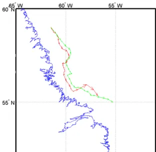
One of the main benefits of the PIC approach is the Lagrangian advection of material. In the ice application, this should allow better

Figure 3: Ice floe trajectory from a beacon (red) and from a model particle. The trajectory starts on 26 January and ends on 3 April. Each vector represents a one-day drift.

prediction of ice edges, and ice trajectories can be simulated by following the movement of individual particles. As an initial indication of model performance, the PIC trajectories are compared with the drift of a single ice beacon for the period 26 January to 3 April, see Fig.3. There is reasonable agreement in the overall shape and length of the trajectories. To quantify this agreement, a sequence of particle trajectories were identified using the daily positions from the beacon as starting points. Fig. 4 shows that the rms error between the beacon and particles increases as a function of the period of the trajectory. The initial rapid increase in error may be indicative of short time scale errors (Tang and Gui, 1996) or space scale errors related to the ocean model resolution (about 18 km). For trajectory periods greater than 4 days, the error continues to increase with trajectory period but at a slower and more consistent rate. These results indicate some

improvement over those derived from the Eulerian model (Fig. 6 – Yao et al 2000) although the simulation year and verification data are different.

(7)

0 20 40 60 80 100 0 5 10 15 20 25 30

Forecast Period (days)

R M SE ( k m )

Figure 4: Root mean square error of simulated trajectory vs. beacon trajectory as a function of forecast period.

CONCLUSION

The new ice dynamics model of the Canadian Ice Service has been described in this paper. The main features of the model include a PIC formulation for ice advection, the viscous plastic rheology of Hibler (1979), and an implicit solution of the momentum equations that follows the general direction of Zhang and Hibler (1997). In particular, the model is implemented using spherical coordinates, which is an important requirement for operational ice forecasting.

Implementation of the model includes interfaces to ocean and thermodynamics models, as well as other environmental data sources. Thus, the present ice dynamics model can run coupled to an ocean model. A seasonal simulation of ice cover along the East Coast of Canada was carried out in order to examine the performance of the model. The results indicate that model performance is appropriate. It is difficult, however, to obtain quantitative estimates of accuracy by comparing the resulting ice thicknesses and volumes with observations. The difficulties are due to the numerous influences introduced by the ocean model and water temperatures.

ACKNOWLEDGEMENTS

The financial support of the Program on Energy Research and Development (PERD) is gratefully acknowledged.

REFERENCES

Blumberg, AF, and Mellor, GL (1987). “A description of a three-dimensional coastal ocean circulation model,” in Three-Dimensional Coastal Ocean Models, Vol 4, ed. N. Heaps, American Geophysical Union, pp.1-16.

Flato, GM (1993). “A Particle-In-Cell sea-ice model,” Atmosphere-Ocean, Vol. 31, No. 3, pp. 339-358.

Hibler, WDIII (1979). “A dynamic thermodynamic sea ice model,” J. Physical Oceanography, Vol. 9, No. 4, pp. 815-846.

Hibler, WDIII (1980). “Modeling a variable thickness sea ice cover,” Monthly Weather Review, Vol 108, pp. 1943-1973.

Hunke, EC, and Dukowicz, JK (1997).“An elastic-viscous-plastic model for sea ice dynamics”, J. Physical Oceanography, Vol. 27, No. 4, pp. 1849-1867.

Huang, ZJ and Savage, SB (1998).“Particle-In-Cell and finite difference approaches for the study of marginal ice zone problems,” Cold Regions Science and Technology, Vol. 26, No 1, pp 1-28.

Mellor, GL (1996). “User’s guide for a three-dimensional primitive equation, numerical ocean model,” Atmospheric and Oceanic Sciences Program, Princeton University, Princeton, N. J., 35 p.

Sayed, M, and Carrieres, T (1999). “Overview of a new operational ice forecasting model,” Proceedings of the 9th International Offshore and Polar Engineering Conference (ISOPE ‘99), Brest, France, Vol. II, pp.622-627.

Tang, CL and Wang, CK (1996). “A gridded data set of temperature and salinity for the northwest Atlantic Ocean,” Canadian Data Reports, Hydrography and Ocean Sciences, No 148, 45 p.

Tang, CL and Gui, Q (1996). “A dynamical model for wind-driven ice motion: application to ice drift on the Labrador Shelf,” J. Geophys. Res. Vol 101, pp. 28,343-28,364.

Thordndike, AS, Rothrock, DA, Maykut, GA, and Colony, R (1975). “The thickness distribution of sea ice,” J. Geophysical Research, Vol. 100, No. C10, pp. 20,601-20,612.

Yao, T, CL Tang, Carrieres, T, and Tran, DH (2000). “Verification of a coupled ice ocean forecasting system for the Newfoundland shelf,” Atmosphere-Ocean, Vol 38, pp. 557-575.

Zhang, J and Hibler, WDIII (1997).”On an efficient numerical method for modelling sea ice dynamics,” J. Geophysical Research, Vol. 102, No. C4, pp. 8691-8702.

APPENDIX A: PARTICLE-IN-CELL FORMULATION

In this formulation, the ice cover is represented by discrete particles that can be advected in a Lagrangian manner. Each particle can be assigned certain attributes. In the present work, each particle is given a volume. In the present model, the volume may change only due to thermodynamic growth and melt. Those are introduced through an interface to a separate thermodynamics program (see the above section on the seasonal simulation). An area and a thickness are also associated with each particle. At each time step, the velocities are mapped from the grid to the particles. Particles are then individually advected. The mass and area of each particle are mapped, from the new positions, back to the grid. At that stage, the areas, and consequently thicknesses, may be adjusted if the concentration (ice area coverage) exceeded unity in any grid cell.

A bilinear interpolation functions is used to map the velocities froim the grid to the particles. Considering particle n to be at location xp, yp, and grid node co-ordinates as (xij, yij), the interpolation coefficients ω would be given by

(8)

⎪⎩

⎪

⎨

⎧

₋ _≤_∆ = ∆ − − ∆ = otherwise x ij x t n p x if n j i x S x n j i x S ij x t n p x x t n p x ij x x 0 ) , ( 1 ) , , ( ) , , ( |] ) , ( | [ )) , ( , ( ω (A.1) and

⎪⎩

⎪

⎨

⎧

₋ _≤_∆ = ∆ − − ∆ = otherwise y ij y t n p y if n j i y S y n j i Sy ij y t n p y y t n p x ij x y 0 ) , ( 1 ) , , ( ) , , ( |] ) , ( | [ )) , ( , ( ω (A.2)

where t is time, and ∆x and ∆y are the grid cell dimensions. The above interpolation functions are used to calculate particle velocities, up and vp , as follows

) , ( )) , ( , ( )) , ( , ( )) , ( ( ), , ( )) , ( , ( )) , ( , ( )) , ( ( j i v t n p y ij y y t n p x ij x x j i t n X p v j i u t n p y ij y y t n p x ij x x j i t n X p u ω ω ω ω ∑ ∑ = ∑ ∑ = (A.3)

To improve the accuracy of the advection, particle positions at half a time step are evaluated as

2 ) ), , ( ( ) , (n t + n t t ∆t =X uX * X (A.4)

The velocities are then mapped again to those particle positions. Finally, particles are advected according to

t t t n t t n, +∆)= ( , )+ ( , )∆ ( X uX* X (A.5)

Bilinear interpolation functions are also used to map the mass and area of each particle to the grid. The concentration of a grid cell c(xij, t) would be given by ∑ ∆ ∆ = n x xij nt y xij nt An t x y t ij x c( , ) ω ( ,X( , ))ω ( ,X( , )) ( , ) 1 (A.6)

where A(n,t) is the area of particle n. The thickness are then calculated as follows ∑ ∆ ∆ = n c xij t x y t n V t n ij x y t n ij x x t ij x h ) , ( 1 ) , ( )) , ( , ( )) , ( , ( ) , ( X X

ω

(A.7) where V(n,t) is the volume of particle n.

APPENDIX B: COEFFICIENTS USED IN THE NUMERICAL

SOLUTION

The coefficients of Eqs (14) and (15) are listed in this Appendix. They are used to solve for the velocities on the grid using Point Successive Over Relaxation (PSOR). It should be noted that with the staggered B-grid, velocities are defined at the nodes. Scalar values, including viscosity coefficients, are defined at cell centers. Thus, for example, the cell with South-West node (i,j) would have the indices (i+1/2 , j+1/2). The coefficients of Eq. (15) are:

( )

⎥

⎦

⎤

⎢

⎣

⎡

+

−

+

−

+

−

+

⎥

⎦

⎤

⎢

⎣

⎡

+

−

+

−

+

−

+

⎥

⎦

⎤

⎢

⎣

⎡

+

−

+

−

+

−

+

⎥

⎦

⎤

⎢

⎣

⎡

+

−

+

−

+

−

+

−

+

−

+

−

+

−

+

=

2 /

1 ,

2 /

1

2 /

1 ,

2 /

1

2 /

1 ,

2 /

1

2 /

1 ,

2 /

1

2

2 tan

2 /

1 ,

2 /

1

2 /

1 ,

2 /

1

2 /

1 ,

2 /

1 ,

2 /

1

4 tan

2 /

1 ,

2 /

1

2 /

1 ,

2 /

1

2 /

1 ,

2 /

1

2 /

1 ,

2 /

1

2

1

2 /

1 ,

2 /

1

2 /

1 ,

2 /

1

2 /

1 ,

2 /

1

2 /

1 ,

2 /

1

2 /

1 ,

2 /

1

2 /

1 ,

2 /

1

2 /

1 ,

2 /

1

2 /

1 ,

2 /

1

2

1 cos

j

i

j

i

j

i

j

i

R

j

i

j

i

j

i

j

i

y

R

j

i

j

i

j

i

j

i

y

j

i

j

i

j

i

j

i

j

i

j

i

j

i

j

i

x

c

u

w

U

w

c

t

ice

mass

ij

a

η

ϕ

η

δ

ϕ

η

δ

ζ

η

ζ

η

ζ

η

ζ

η

δ

β

ρ

δ

λ

r

(B.1)

( )

⎥⎥ ⎦ ⎤ ⎢ ⎢ ⎣ ⎡ + − + + − + − − + − − = 2 / 1 , 2 / 1 2 / 1 , 2 / 1 2 / 1 , 2 / 1 2 / 1 , 2 / 1 2 2 1 , j i j i j i j i x j i b

ζ

η

ζ

η

δ

λ

(B.2)

( )

⎥⎥ ⎦ ⎤ ⎢ ⎢ ⎣ ⎡ + + + + + + − + + − + = 2 / 1 , 2 / 1 2 / 1 , 2 / 1 2 / 1 , 2 / 1 2 / 1 , 2 / 1 2 2 1 , j i j i j i j i x j i c

ζ

η

ζ

η

δ

λ

(B.3)

( )

⎥

⎦

⎤

⎢

⎣

⎡

+

−

+

−

+

−

⎥⎦

⎤

⎢⎣

⎡

+

−

+

⎥⎦

⎤

⎢⎣

⎡

+

−

+

−

+

=

2 /

1 ,

2 /

1

2 /

1 ,

2 /

1

2 /

1 ,

2 /

1

2 /

1 ,

2 /

1

4 tan

2 /

1 ,

2 /

1

2 /

1 ,

2 /

1

4 tan

2 /

1 ,

2 /

1

2 /

1 ,

2 /

1

2

1 ,

j

i

j

i

j

i

j

i

y

R

j

i

j

i

y

j

i

j

i

y

j

i

d

η

δ

ϕ

η

δ

ϕ

η

δ

λ

(B.4)

(9)

( )

⎥

⎦

⎤

⎢

⎣

⎡

+

−

+

−

+

−

⎥⎦

⎤

⎢⎣

⎡

−

+

−

+

⎥⎦

⎤

⎢⎣

⎡

−

+

−

+

=

2 /

1 ,

2 /

1

2 /

1 ,

2 /

1

2 /

1 ,

2 /

1

2 /

1 ,

2 /

1

4 tan

2 /

1 ,

2 /

1

2 /

1 ,

2 /

1

4 tan

2 /

1 ,

2 /

1

2 /

1

2 /

1 ,

2 /

1

2

1 ,

j

i

j

i

j

i

j

i

y

R

j

i

j

i

y

j

i

j

i

y

j

i

e

η

δ

ϕ

η

δ

ϕ

η

δ

λ

(B.5)

The coefficients of Eq. (16) are:

( )

⎥ ⎥ ⎦ ⎤ ⎢ ⎢ ⎣ ⎡ + − + + + + − + + − − + ⎥ ⎥ ⎥ ⎥ ⎥ ⎦ ⎤ ⎢ ⎢ ⎢ ⎢ ⎢ ⎣ ⎡ + − − + − + + + − + + + − + + − + − − − + − − − + ⎥ ⎥ ⎦ ⎤ ⎢ ⎢ ⎣ ⎡ + − + + + + − + + − − + ⎥ ⎥ ⎥ ⎥ ⎥ ⎦ ⎤ ⎢ ⎢ ⎢ ⎢ ⎢ ⎣ ⎡ + − + + − + + + + + + + − + + − + + − − + − − + − + = 2 / 1 , 2 / 1 2 / 1 , 2 / 1 2 / 1 , 2 / 1 2 / 1 , 2 / 1 2 2 2 tan 2 / 1 , 2 / 1 2 / 1 , 2 / 1 2 / 1 , 2 / 1 2 / 1 , 2 / 1 2 / 1 , 2 / 1 2 / 1 , 2 / 1 2 / 1 , 2 / 1 2 / 1 , 2 / 1 4 tan 2 / 1 , 2 / 1 2 / 1 , 2 / 1 2 / 1 , 2 / 1 2 / 1 , 2 / 1 2 2 1 2 / 1 , 2 / 1 2 / 1 , 2 / 1 2 / 1 , 2 / 1 2 / 1 , 2 / 1 2 / 1 , 2 / 1 2 / 1 , 2 / 1 2 / 1 , 2 / 1 2 / 1 , 2 / 1 2 2 1 cos j i j i j i j i R j i j i j i j i j i j i j i j i y R j i j i j i j i x j i j i j i j i j i j i j i j i y c u w U w w c t ice mass ij a η η η η ϕ η ζ η ζ η ζ η ζ δ ϕ η η η η δ ζ η ζ η ζ η ζ η δ β ρ δ ϕ r (B.6)

( )

⎥

⎦

⎤

⎢

⎣

⎡

+

−

+

−

=

2 /

1 ,

2 /

1

2 /

1 ,

2 /

1

2 cos

2

1 ,

j

i

j

i

x

j

i

b

η

ϕ

δ

ϕ

(B.7)

( )

⎥

⎦

⎤

⎢

⎣

⎡

+

−

+

=

2 /

1 ,

2 /

1

2 /

1 ,

2 /

1

2 cos

2

1 ,

j

i

j

i

x

j

i

c

η

ϕ

δ

ϕ

(B.8)

( )

⎥

⎦

⎤

⎢

⎣

⎡

+

−

+

−

+

−

⎥

⎦

⎤

⎢

⎣

⎡

+

−

+

−

+

−

+

⎥

⎦

⎤

⎢

⎣

⎡

+

−

+

−

+

−

+

−

+

=

2 /

1 ,

2 /

1

2 /

1 ,

2 /

1

2 /

1 ,

2 /

1

2 /

1 ,

2 /

1

4 tan

2 /

1 ,

2 /

1

2 /

1 ,

2 /

1

2 /

1 ,

2 /

1

2 /

1 ,

2 /

1

4 tan

2 /

1 ,

2 /

1

2 /

1 ,

2 /

1

2 /

1 ,

2 /

1

2 /

1 ,

2 /

1

2

1 ,

j

i

j

i

j

i

j

i

y

R

j

i

j

i

j

i

j

i

y

R

j

i

j

i

j

i

j

i

y

j

i

d

η

δ

ϕ

η

ζ

η

ζ

δ

ϕ

η

ζ

η

ζ

δ

ϕ

(B.9)

( )

⎥

⎦

⎤

⎢

⎣

⎡

+

−

+

−

+

−

+

⎥

⎦

⎤

⎢

⎣

⎡

−

+

−

+

−

+

⎥

⎦

⎤

⎢

⎣

⎡

−

+

−

+

−

+

−

+

=

2 /

1 ,

2 /

1

2 /

1 ,

2 /

1

2 /

1 ,

2 /

1

2 /

1 ,

2 /

1

4 tan

2 /

1 ,

2 /

1

2 /

1 ,

2 /

1

2 /

1 ,

2 /

1

2 /

1 ,

2 /

1

4 tan

2 /

1 ,

2 /

1

2 /

1 ,

2 /

1

2 /

1 ,

2 /

1

2 /

1 ,

2 /

1

2

1 ,

j

i

j

i

j

i

j

i

y

R

j

i

j

i

j

i

j

i

y

R

j

i

j

i

j

i

j

i

y

j

i

e

η

δ

ϕ

η

ζ

η

ζ

δ

ϕ

η

ζ

η

ζ

δ

ϕ

(B.10)

Note that the right-hand-sides of Eqs (15) and (16) consist of the driving forces ans a few terms that are evaluated from the velocities calculated at the previous time step. Those terms are calculated using standard central finite difference, and are not listed here.