FIERAsystem theory documentation: smoke movement model

Publisher’s version / Version de l'éditeur:

Vous avez des questions? Nous pouvons vous aider. Pour communiquer directement avec un auteur, consultez la première page de la revue dans laquelle son article a été publié afin de trouver ses coordonnées. Si vous n’arrivez pas à les repérer, communiquez avec nous à PublicationsArchive-ArchivesPublications@nrc-cnrc.gc.ca.

Questions? Contact the NRC Publications Archive team at

PublicationsArchive-ArchivesPublications@nrc-cnrc.gc.ca. If you wish to email the authors directly, please see the first page of the publication for their contact information.

https://publications-cnrc.canada.ca/fra/droits

L’accès à ce site Web et l’utilisation de son contenu sont assujettis aux conditions présentées dans le site LISEZ CES CONDITIONS ATTENTIVEMENT AVANT D’UTILISER CE SITE WEB.

Internal Report (National Research Council of Canada. Institute for Research in Construction), 2002-01-01

READ THESE TERMS AND CONDITIONS CAREFULLY BEFORE USING THIS WEBSITE. https://nrc-publications.canada.ca/eng/copyright

NRC Publications Archive Record / Notice des Archives des publications du CNRC :

https://nrc-publications.canada.ca/eng/view/object/?id=05cb8624-66d0-4cd4-af06-3edb4ea7246e https://publications-cnrc.canada.ca/fra/voir/objet/?id=05cb8624-66d0-4cd4-af06-3edb4ea7246e

NRC Publications Archive

Archives des publications du CNRC

For the publisher’s version, please access the DOI link below./ Pour consulter la version de l’éditeur, utilisez le lien DOI ci-dessous.

https://doi.org/10.4224/20386250

Access and use of this website and the material on it are subject to the Terms and Conditions set forth at

FIERAsystem theory documentation: smoke movement model

Smoke Movement Model

Fu, Z.; Kashef, A.; Bénichou, N.; Hadjisophocleous, G.

IR-835

FIERA

system

Theory Documentation

SMOKE MOVEMENT MODEL

Zhuman Fu, Ahmed Kashef, Noureddine Benichou,

and George Hadjisophocleous

Internal Report No.

Date of Issue: March 2002

This is an internal report of the Institute for Research in

Construction. Although not intended for general distribution, it

may be cited as a reference in other publications.

THEORY OF SMOKE MOVEMENT MODEL

Zhuman Fu, Ahmed Kashef, Noureddine Benichou and George

Hadjisophocleous

TABLE OF CONTENTS

TABLE OF CONTENTS... i SUMMARY... 1 NOMENCLATURE ... 2 1. INTRODUCTION... 7

1.1 Assumptions and Limitations... 8

2. DERIVATION OF GOVERNING EQUATIONS ... 10

3. COMBUSTION AND CHEMISTRY... 15

3.1 Heat Release Rate... 15

3.2 Combustion Chemistry... 17

3.3 Calculation of (∆Η)O or (∆Η)F... 20

4. FLUID FLOW ... 22

4.1 Plume Entrainment ... 22

4.2 Door/Window Vent Flow... 23

4.3 Ceiling Vent Flow ... 27

4.4 Mechanical Ventilation ... 29

4.5 Stair Shaft Flow... 31

4.6 Species Concentration ... 33

5. HEAT TRANSFER ... 34

5.1 Conduction Heat Transfer ... 34

5.2 Convection Heat Transfer in Non-Fire Rooms ... 34

5.3 Ceiling Jet-Induced Heat Transfer ... 36

5.4 Convection Heat Transfer in Fire Rooms ... 38

5.5 Radiation Heat Transfer ... 38

5.5.1 Derivation of Equations ... 38

5.5.2 Calculation of View Factors... 41

5.5.3 Gas Emissivity... 42

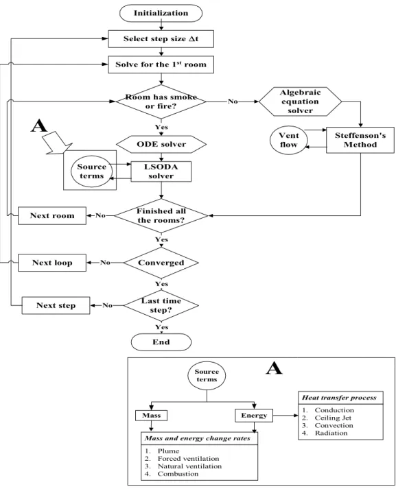
6. NUMERICAL METHOD... 44

6.1 Introduction ... 44

6.2 Numerical Properties of the ODE System... 46

6.2.1 Stiff Equations... 47

6.2.2 BDF Method... 47

6.2.3 Error Estimation and Automatic Control of Step Size and Order... 48

6.3 Solution of the Constant Temperature Compartments... 49

6.4 Solution of the Physical Sub-models ... 50

6.4.1 Conduction ... 50

6.4.2 Ceiling Jet Heat Transfer... 53

7. VERIFICATION EXAMPLES... 54

7.1 Standard Single Compartment ... 54

Analysis of the Results... 54

7.2 One-Compartment with Mechanical Ventilation ... 56

Analysis of the Results... 58

7.3 Two Compartments ... 61

Analysis of the Results... 61

8. REFERENCES ... 64

List of Tables

Table 2.1 A List of the Governing Ordinary Differential Equations ... 13

Table 7.1 Zone Model Input Data for Single Compartment Example ... 55

Table 7.2 Comparison of Model Prediction with Reference [59]... 56

Table 7.3 Basic Input Data of the Test Facility... 58

Table 7.4 Results of Test 1 with Mechanical Ventilation ... 59

Table 7.5 Results of Test 2 with Mechanical Ventilation ... 60

Table 7.6 Results of Test 3 with Mechanical Ventilation ... 60

Table 7.7 Zone Model Input Data for Two-Compartment Example... 61

List of Figures

Figure 4.1 Basic vertical-vent (door/window) configuration... 24

Figure 4.2 Possible neutral planes in an opening ... 25

Figure 4.3 Basic horizontal-vent (ceiling vent) configuration ... 27

Figure 4.4 Schematic of the mechanical ventilation opening ... 30

Figure 4.5 Schematic of an effective ceiling vent for a stair shaft... 31

Figure 5.1 Schematic of the radiation geometry ... 39

Figure 5.2 A schematic of flame radiation to a rectangular surface ... 42

Figure 6.1 Schematic Chart of Numerical Calculation ... 45

Figure 7.1 Schematic of the Test Facility ... 57

Figure 7.2 Predicted and Experimental Results for Pressure Difference Between the Burn Room and Corridor Near the Ceiling ... 62

Figure 7.3 Predicted and Experimental Results for Averaged Gas Temperature of Burn Room (BR) and Corridor (CR)... 62

Figure 7.4 Predicted and Experimental Results for the Interface Heights of the Burn Room (BR) and Corridor (CR)... 63

SUMMARY

This report describes a two-zone model developed at the National Research Council of Canada (NRC) to predict fire growth and smoke production and movement in a multi-compartment building. The development of this model is primarily intended to help evaluate the risk from fires in buildings. This report describes the theoretical physical models, numerical methods, and also presents some verification examples.

The report describes the derivation of the whole set of the governing ordinary differential equations (ODE). The selected independent governing variables for each compartment are pressure, enthalpy of upper layer, and mass of upper and lower layers. The

implemented fire physical sub-models are described; including combustion and chemistry model, fluid flow model and heat transfer model. The combustion and chemistry model includes the calculation of heat release rate and species production and consumption rates, while the fluid flow model includes the calculation of plume entrainment,

door/window type vent flow, ceiling vent flow, mechanical ventilation, stair shaft flow, and species transport. The heat transfer model includes the calculation of heat

conduction, heat convection, ceiling jet-induced heat convection, and radiation heat transfer.

The numerical method used to solve the system of governing equations is presented. Backward differentiation formulas (BDFs) method has been used to solve the stiff ODE system. Some details about the ODE solver are presented, including the basic properties of stiff equations, basic algorithm of the BDF method and the control mechanism of precision criteria, step size and order. The method of solving the constant temperature compartments is also presented. Besides, the method applied to solve the

one-dimensional conduction partial differential equation is described, including discrete equations and Tri-Diagonal Matrix Algorithm (TDMA) method. The numerical method of calculating ceiling jet-induced convection heat transfer is also given.

Three sets of experimental data for single and two-compartment fire tests with and without mechanical ventilation are compared to the predictions of the model. The comparison shows that the model predictions compare favorably with the experimental data, especially the upper layer gas temperature, interface height, neutral plane height, and vent flow rate. The model, however, over-predicts the floor incident radiant heat flux and the lower wall surface temperature, and under-predicts the lower layer gas

temperature.

NOMENCLATURE

A Area

i

Ae Effective orifice area on the ith floor Aint Area of interface

S

A Cross-sectional area of stair shaft AV Vent area

Aw Surface area of a wall, ceiling or floor

I

Bi Biot number of the inside surface of a wall O

Bi Biot number of the outside surface of a wall C Specific heat

Cconv A coefficient in the convection heat transfer formula

CCV Coefficient of ceiling vent flow

CE1, CE2 Coefficients in McCaffrey’s plume entrainment correlation

CLOL Lower oxygen limiting coefficient

CP Specific heat at constant pressure

Csoot Volume fraction of soot in smoke layer

CV Specific heat at constant volume

Cvent Coefficient of door/window type vent flow e

D Equivalent diameter

i

d Density of people on the stairs between the ith floor and (i-1)th floor E Internal energy

Fkj Configuration factor from surface k to surface j for radiation

Fo Fourie number

FOP Fuel to oxygen ratio in fire plume

FOS Stoichiometric fuel to oxygen ratio

Fr Froude number

g Gravitational acceleration Gr Grashof number

H Vertical distance between the fire source and ceiling h Heat transfer coefficient

h~ Characteristic heat transfer coefficient i

H Gas enthalpy of layer I

i

h Height of stair shaft between the ith floor and (i-1)th floor

hIC, hOC Convection heat transfer coefficients of the inside and outside surface of a

wall, ceiling or floor

(∆H)F Heat of combustion per unit mass of fuel

(∆H)O Heat of combustion per unit mass of oxygen

∑

H&si Rate of net enthalpy gain of layer i by mass flow across its boundary

K Conductivity

k Friction pressure loss coefficient

L Thickness of a wall, ceiling or floor

Le Equivalent mean beam length of smoke layer for radiation m Mass

AV

m& Average vent mass flow rate

BF

m Mass of the burned fuel

main

BF

m Main part of the burned fuel

min

BF

m Minimal part of the burned fuel

C

m Mass of carbon in fuel

CO m Mass production of CO 2 CO m Mass production of CO2 CRP

m Mass production of carbon-related products (Soot+CO+CO2) e

m& Mass entrainment rate

Fan

m& Specified mass exhaust rate of the fan

H

m Mass of hydrogen in fuel

O H2

m Mass production of water

max

m& Maximum smoke exhaust rate from the upper layer

ML

m& Mass flow rate exhausted from lower layer

MU

m& Mass flow rate exhausted from upper layer

O

m Mass of oxygen in fuel

2

O

m Oxygen consumption from air in combustion

PF

m Mass of fuel pyrolysis

main

PF

m Mass production of the main part of fuel

min

PF

m Mass production of the minimal part of fuel

soot

m Mass production of soot

1 tox

m Mass of the first kind of toxic species of mPFmin

2 tox

m Mass of the second kind of toxic species of mPFmin

3 tox

m Mass of the third kind of toxic species of mPFmin TUCF

m Mass of the total unburned combustible fuel

UF

m Mass of the unburned fuel

main

UF

m Main part of the unburned fuel

min

UF

m Minimal part of the unburned fuel

∑

m&e Net mass flow rate entering a layer by plume entrainment

∑

m&e,K Net mass flow rate of species K entering a layer by plume entrainment

∑

m&si Net mass gain rate of layer i by mass flow through its boundary

∑

m&V Net mass flow rate entering a layer by vent flow

∑

m&V,K Net mass flow rate of species K entering a layer by vent flow

NS Number of species Nu Nusselt number P Pressure

Pb Pressure difference at the bottom position

2 CO P Partial pressure of CO2 Pg Gas pressure O H2

P Partial pressure of water vapour Pr Prandtl number

Pt Pressure difference at the top position

P1(Z), P2(Z) Pressures of the two sides of a vertical-vent at height Z

∆PF Compartment floor pressure difference relative to ambient

∆P(Z) Pressure difference between the two sides of a vertical-vent at height Z Q Heat release rate

Q′ Equivalent heat release rate considering upper layer effect on ceiling jet Qc Convection heat release rate

Qceil, qceil Convection heat loss and flux to ceiling surface

Qconv, qconv Convection heat loss and flux to a surface of a wall, ceiling or floor

* eq

Q Dimensionless heat release rate at the interface QF Heat release rate directly radiated out of the fuel

* H

Q Dimensionless heat release rate

i

q Net radiation heat transfer rate of surface i

IF

q Average radiant incident heat flux to a compartment floor

IR

q Net radiation heat flux to the inside surface of a wall, ceiling or floor

N

Q Nominal heat release rate of the fuel

OR

q Net radiation heat flux to the outside surface of a wall, ceiling or floor

∑

Qsi Net heat gain rate of layer i by heat transfer or combustion

R Gas constant

r Radial distance from the stagnation point on the ceiling surface RC Radius of the circular equivalent ceiling surface

ReH Reynolds number i

S& Net energy gain rate of layer i as a source term T Temperature

t Time

∆t Time step size

Ta Ambient temperature

Tad Adiabatic ceiling jet temperature

Tceil Ceiling surface temperature

TFLR Compartment averaged floor interior surface temperature

Tg Gas layer temperature

TI Assumed interface temperature

Tw Surface temperature of a wall, ceiling or floor

TWL Compartment averaged lower wall interior surface temperature

TWU Compartment averaged upper wall interior surface temperature

T(x, 0) Initial temperature profile of a wall, ceiling or floor V Volume

VEX, MX Maximum exchange volume flow rate

Fan

V& Specified volume exhaust rate of the fan

VH Volumetric flow rate from high to low-pressure side

VL Volumetric flow rate from low to high-pressure side

ML

V& Volume flow rate exhausted from lower layer

MU

V& Volume flow rate exhausted from upper layer VN Net volumetric flow rate

x Spatial coordinate in heat conduction equation ∆x Space step size

YK Mass fraction of species K

YLOL Lower oxygen limiting mass fraction

2

O

Y Oxygen mass fraction Z Height

Zceil Ceiling height

Ze Plume entrainment height

Zext Mechanical ventilation opening extension

Zfire Height of burner’s surface

Zf1, Zf2 Floor elevation of the two compartments connected by a vertical-vent

ZI Height of interface of upper layer and lower layer

ZN Neutral plane elevation of a vertical-vent flow

ZS Thickness of smoke layer

Zsi Sill height

Zso Soffit height

Z12 Entrainment height of vent flow-induced plume

Greek Symbols

Γ Perimeter of stair shaft

ρ Mass density

β Tread coefficient of stair shaft

γ Ratio of specific heats

γC/CRP Mass ratio of the carbon in the CRP products to the total CRP products

γCO Mass ratio of CO production to carbon-related products (CO+CO2+Soot)

γsoot Mass ratio of soot production to carbon-related products

2

CO

ε Emittance of CO2

εD Emittance reduction resulting from spectral overlap

εg Gas total emittance

O H2

ε Emittance of water vapour

εj Emissivity of surface j

εsoot Emittance of soot

σ Stephen Boltsman constant

ν Kinematic viscosity

δkj Kronecker function

τkj Radiation transmittance from surface k to surface j

αkj Radiation absorptance from surface k to surface j

φ Equivalence ratio

χC Mass fraction of carbon in the fuel

χH Mass fraction of hydrogen in the fuel

χtox1 Mass ratio of the first kind of toxic species production to fuel pyrolysis

χtox2 Mass ratio of the second kind of toxic species production to fuel pyrolysis

χO Mass fraction of oxygen in the fuel

Π Dimensionless pressure difference

i

Ω& Net mass gain rate of layer i by mass flow through its boundary

Subscripts

U, L Upper, lower layer

H, L Higher or lower pressure side FL Flooding condition T, B Top, bottom sides

1, 2, F Upper surface, lower surface, flame in radiation formula

1. INTRODUCTION

Computational modeling of fire in a compartment can be achieved either using a zone modeling approach or a field modeling method. In this study, the zone modeling approach was used in which the gas within each compartment is generally divided into one, or a few, control volumes (zones), and for each zone, the physical parameters such as gas temperature and species concentrations are assumed to be spatially uniform. Then, from the mass and energy conservation principle, as well as the ideal gas law, a set of ordinary differential equations (ODE) is derived. In this type of model, the physical details of the gas within a zone are not considered, however mass and energy transport between zones has to be calculated by modeling the relevant fire sub-processes: combustion and chemistry, fluid flow and heat transfer. [1-6]

Zone models may be grouped into two types based on the number of control volumes (zones) in each compartment: one-zone models and two-zone models. One-zone models are widely used in the analysis of post-flashover fires, as well as smoke movement in the compartments remote from the fire room (network models). Two-zone models divide the gas in a compartment into two distinct zones: an upper, higher temperature zone and a lower, lower-temperature zone. These zones are a result of buoyancy-induced thermal stratification. Two-zone models can be used to analyze pre-flashover fires, and some models of this type have been developed. [7-9] A comprehensive review of existing fire models can be found in Friedman. [7]

The one-zone modeling concept dates back to the work of Kawagoe, who developed a single-zone approach for analyzing a post-flashover fire. [10] This approach was the basis of the development of a series of single-zone post-flashover fire models. [11] The

application of the two-zone concept was pioneered by Thomas, Hinkley, Theobald, and Simms, who constructed a steady state, two-layer model for calculating the flow of smoke through roof vents.[11-13] Before the mid-1970s, however, fire modeling research was focussed on post flashover fires; i.e., fully developed fires, using the one-zone method.[14]

Quintiere has mentioned that the two-zone fire modeling of pre-flashover fires emerged in the mid-1970s with the publication of a basis for the zone model approach by Fowkes in his work with Emmons.[5, 15] Almost simultaneously, several zone computer models were produced by Quintiere, Pape and Walterman and Mitler working with Emmons.[5,

16-18]

In the late 1970s the first Harvard model and code was completed by Emmons and Mitler, which might be the first comprehensive room fire model for one compartment.[18,

19]

However, the first true multi-compartment model of this type was formulated by Tanaka.[1, 20] Zone modeling work continued, especially at NIST, where models such as FIRST, FAST, CCFM and CFAST were developed.[21-23] Jones, Jones and Forney, and

Peacock and Forney developed the CFAST model based on FAST and CCFM, in which the governing equation set is formulated to allow the actual physical phenomena to be taken as source terms. This allows the greatest flexibility in modifying the terms that are appropriate to the problem being solved.[1-3] In the CFAST model, the conservation equations are solved in their original differential form, and the pressure is not assumed to be steady state, nor the lower layer temperature to be at ambient conditions.

NRC has been conducting research work on fire risk evaluation of buildings which has resulted in a comprehensive fire risk evaluation model FiRECAMTM for residential and office buildings.[24-26] Currently, research on fire risk evaluation of light industrial

buildings is being undertaken, which is used to develop a system model called FIERA.[27] As part of the FIERAsystem, the model described in this report will be used to calculate smoke movement in industrial buildings, as well as to improve the calculation of smoke movement in office and residential buildings.

Based on similar concepts used by CFAST, a two-zone model has been developed to predict smoke and fire development in buildings. Both the model and interface are coded using MS Visual Basic Version 5. This model uses a new form of the governing ordinary differential equations and fire sub-models. The following sections present the governing equation set for this model and describe the fire sub-models, including fire growth, fluid flow, and heat transfer models.

1.1 Assumptions and Limitations

The developed smoke model uses mainly the principal laws of thermodynamics

(conservation of mass, energy, and momentum) to simulate the important time-dependent phenomena involved in fires. However, in areas where knowledge is not available, empirical correlations (when data are available) or even reasonable guesses were used. The user should be aware of these limitations. Following is an overview of the

assumptions and limitations implicit with the current model:

• The model does not include a fire growth model. Rather, the fire is specified by the user in terms of rates of energy and mass released by the burning objects. Such data can be obtained from measurements taken in large or small-scale calorimeters. It is the responsibility of the user to provide the appropriate rates, which depend on the of problem under consideration.

• The entrainment coefficients are empirically determined values. These values are mainly relevant for models up to a three-compartment case. For a larger number of rooms, more data are needed. In these situations, the entraiment values may

introduce some effects on the fire plume or on hot gases flow from fire origin room to the neighboring rooms.

• Each layer is assumed to be of uniform temperature, density, and species concentrations. This assumption implies that the moment the hot gases enter a

compartment, the model calculates a hot gas layer that covers the entire ceiling. If the

hot gases entered a large room from one end, the model would predict that the temperature at the far end would immediately increase. In other words the transient time to fill the area is not considered. In real cases, there would be a delay time as the hot gases travel across the large room.

2. DERIVATION OF GOVERNING EQUATIONS

Following the two-zone modeling concept, each compartment is divided into two zones. For each zone, the mass, internal energy, enthalpy, density, temperature and volume are denoted as mi, Ei, Hi, ρi, Ti and Vi, respectively, where i=U refers to the upper layer, and i=L refers to the lower layer. The thermodynamic pressures for the upper and lower

layers, PU and PL are assumed to be identical and are denoted as P. Using thermodynamic relations and definitions as well as the ideal gas law, the following equations are given:

Vi m_i i = ρ (2.1) i i V i C mT E = (2.2) H_i =E_i +PV_i T_i (2.3) P= ρ_iR (2.4) L U V V V = + (2.5)

CP and CV, specific heats at constant pressure and volume, are assumed to be constant for the gas in the upper and lower layers, and the following relation exists:

V P V P C R C C C = − = / , γ (2.6)

where R is the gas constant. Applying Equations (2.1) through (2.5) to both the upper and

lower layers in a compartment results in 9 independent algebraic equations with 13 variables. To close the equation set, four additional independent equations are needed, which can be obtained by applying mass and energy conservation principles to each zone. The resulting equations are as follows:

Mass conservation:

∑

= _si i _m dt dm & (2.7)

Energy conservation (First Law):[28]

∑

+

∑

= + si si i i _{H Q} dt dV P dt dE _& (2.8) 10

where

∑

m&_si is the net mass gain rate of layer i by mass flow across the boundary,

∑

H&si is the rate of the net enthalpy gain of layer i by mass flow across the boundary,

∑

Qsi is the rate of net heat gain of layer i by heat transfer or combustion.

Thus, the whole equation set has been closed. To facilitate the solution, the above system of ODEs can be converted into other forms as given below.

Let us denote:

∑

= Ω&i m&si (2.9)

∑

+

∑

= si si i H Q S& & (2.10)

Following the approach used in CFAST, Ω&_iand S&_i are considered to be source terms. From Equations (2.7) and (2.8) we have:

i i dt dm Ω = & (2.11) i i i _S dt dV P dt dE _& = + (2.12)

Adding the Term

dt dP

i

V to the two sides of Equation (2.12), and considering Equation (2.3), we get: dt dP V S dt dH i i i = & + _(2.13)

Adding the upper and lower layer versions of Equation (2.13), we have:

dt dP V S S dt H H d U L L U + ) =₍ + ₎+ ( _{& &} (2.14)

From Equations (2.1), (2.2), (2.3), (2.4) and (2.6), we have:

P V R C H P _i i = (2.15) 11

Adding the upper and lower layer versions of Equation (2.15), and substituting into (2.14), we get: ) ( 1 L U S S V dt dP _{& &} + − =γ (2.16)

Differentiating equation (2.15), we have:

) ( dt dV P dt dP V R C dt dH _i i P i = + (2.17)

Substitute Equation (2.17) into (2.13), we obtain:       _{− −} = dt dP V S P dt dV i i i 1 ₍γ ₁₎& γ (2.18)

From Equations (2.1), (2.11) and (2.18), and applying the quotient rule to               = i i i V m dt d dt dρ , we obtain:       − + Ω − − = dt dP V T C S V T C dt d _i i i P i i i P i 1 ) ( 1 γ ρ _{& &} (2.19)

Similarly, applying the quotient rule to _           = i i R P dt d dt dT ρ 

 , from Equations (2.4) and (2.19), we obtain:       _{− Ψ +} = dt dP V T C S V C dt dT i i i P i i i P i 1 ₍& & ₎ ρ (2.20) 12

Table 2.1 A List of the Governing Ordinary Differential Equations Variables Equations Mass i i dt dm Ω = & Pressure ) ( 1 L U S S V dt dP _{& &} + − =γ Volume       _{− −} = dt dP V S P dt dV i i i 1 ₍γ ₁₎& γ Density       − + Ω − − = dt dP V T C S V T C dt d i i i P i i i P i 1 ) ( 1 γ ρ _{& &} Temperature       _{− Ψ +} = dt dP V T C S V C dt dT i i i P i i i P i 1 ₍& & ₎ ρ Internal Energy       ₊ = dt dP V S dt dE i i i & γ 1 Enthalpy dt dP V S dt dH i i i = & +

The complete list of equations derived is shown in Table 2.1, which includes equations of mass, pressure, volume, density, temperature, internal energy and enthalpy. To close the system of equations, we only need four independent differential equations. There are many ways to select four independent governing variables from the above list. For example, CFAST selects P, VU, TU and TL as its governing variables. In this model, the equations of pressure, upper layer enthalpy, upper layer mass and lower layer mass are used as follows: ) ( 1 L U S S V dt dP ₌γ − _{& + &} (2.21) dt dP V S dt dH U U U = & + (2.22) U U dt dm Ω = & _(2.23) 13

L L dt dm Ω = & (2.24)

In the literature[1, 3, 29], the two terms on the right side of Equation (2.8) were combined as one term, called enthalpy or total enthalpy. This could result in a little confusion between this term and the real thermodynamic enthalpy term. Thus in this derivation, the equation for thermodynamic layer enthalpy has been given as a complementary to the table

“Conservative Zone Modeling Differential Equations” appearing in references [1, 3, 29], although Hi is directly proportional to Ei by γ in this case.

3. COMBUSTION AND CHEMISTRY

3.1 Heat Release Rate

The heat release rate of combustion can be obtained by:

F PF

N m H

Q = & (∆ ) (3.1)

where QN is the nominal heat release rate,

F

H )

(∆ is the effective heat of combustion per unit mass of fuel which is obtained from experimental data,

PF

m& is the mass pyrolysis rate.

Following the oxygen consumption principle, the oxygen consumption rate needed to release energy of QN assuming no oxygen in the fuel, can be obtained using: [30, 31]

O N O H Q m ) ( 2 = ∆ & (3.2)

where ( is the heat of combustion per unit mass of oxygen. For complex fuels, it could be taken as 13.2 MJ/kg

o

H)

∆

[32]

, while, for simple chemical formula fuels, it can be obtained from the heat of combustion per unit mass of fuel.

The stoichiometric fuel to oxygen ratio, FOS, is:

F O O PF S H H m m FO ) ( ) ( 2 ∆ ∆ = = & & (3.3)

The actual fuel to oxygen ratio in the fire plume is:

2 O e PF P Y m m FO & & = (3.4)

where is the mass entrainment rate of the plume, and Y is the oxygen mass fraction. Thus the equivalence ratio, φ, is:

e

m& O₂

2 ) ( ) ( O e O PF F S P Y m H m H FO FO & & ∆ ∆ = = φ (3.5)

The actual heat release rate is considered to be related to φ as follows:

N

Q f

Q= (φ) (3.6)

In this model, f(φ) is obtained using the following simple relation used by CFAST: [3]

) 1 , max( 1 ) ( φ φ = f (3.7)

The fuel rich flammability is given by a limiting oxygen mass or volume fraction. In order to make the calculation smooth near the fuel rich limit, following the CFAST approach, a limiting coefficient CLOL is introduced: [3]

(

)

[

]

2 1 4 800 2 − − + = O LOL LOL Y Y Tanh C (3.8)

where Tanh(x) is the hyperbolic tangent function of x, and YLOL is the limiting oxygen mass fraction.[33] Thus Equation (3.5) should be adjusted as follows:

LOL O e O PF F C Y m H m H 2 ) ( ) ( & & ∆ ∆ = φ (3.9)

The actual fuel consumption rate can be obtained as follows:

F BF H Q m ) (∆ = & (3.10)

And the oxygen consumption rate from air can also be obtained as follows:

O O H Q m ) ( 2 = ∆ & (3.11)

This model is similar to CFAST’s but re-expressed based on the concept of the equivalence ratio φ.

3.2 Combustion Chemistry

In this model, the global combustion chemistry is written as follows:

O H soot CO CO TUCF tox tox tox O PF m m m m m m m m m m 2 2 2 → 1+ 2 + 3+ + + + + + (3.12)

where m_PF is the mass of the pyrolyzed fuel, which is a user input,

2

O

m is the mass consumption of oxygen, obtained from Equation (3.11) 1

tox

m is the mass production of the first kind of toxic species,

2

tox

m is the mass production of the second kind of toxic species,

3

tox

m is the mass production of the third kind of toxic species,

TUCF

m is the mass production of the total unburned combustible fuel,

2

CO

m is the mass production of carbon dioxide,

CO

m is the mass production of carbon monoxide,

soot

m is the mass production of soot,

O H

m

2 is the water production.

The pyrolyzed fuel is assumed to be composed of two parts: the combustible main part and the incombustible minimal part .

PF m main PF m m_PFmin min PF PF PF m m m main + = (3.13) main PF

m is the mass of the elements, carbon, hydrogen and oxygen of the pyrolyzed fuel:

O H C PF m m m m main = + + (3.14) min PF

m is assumed to be composed of some harmful species, such as hydrogen chloride and hydrogen cyanide, whose mass is much less than the total fuel mass and will not be involved in the further combustion process. Thus from in the left side of Equation (3.12) will directly go into its right side. In this model, can be composed of as many as three kinds of toxic species: , and .

min PF m 2 tox m PF m m 3 min PF 1 tox m m_tox 3 2 1

min tox tox tox

PF m m m

m = + + (3.15)

The mass production of carbon dioxide, carbon monoxide and soot are combined to be one new term m_CRP, carbon-related products as follows:

soot CO CO CRP m m m m = + + 2 (3.16)

where soot is assumed to be composed of carbon.

In terms of fuel consumption, can be divided into two parts: burned pyrolyzate , and unburned pyrolyzate . Both and have the same composition as m . And the main part of will form the term , while the main part of will go into the water and carbon-related products.

PF m m_BF PF UF m m_BF m_UF TUCF m UF m m_BF

The approach in which that is assumed to have the same element composition as the main part of the pyrolyzate, will simplify the calculation of oxygen consumption, although the unburned products of organic fuel are generally hydrocarbons without oxygen content.

TUCF

m

The above chemical equations can be integrated as the following single equation:

(

)

(

)

[

]

(

BF UF

)

TUCF

(

UF

)

CRP

(

CO CO soot

)

HO PF O UF UF UF BF BF BF PF m m m m m m m m m m m m m m m m m m main main main 2 2 min min min 2 min min + + + + + + → + + + + (3.17)

The following part will present the calculation formulas of the combustion chemistry. The composition of the pyrolyzed fuel is defined by the following five mass ratios, which are input by the user of the model.

PF C C =m /m χ (3.18) PF H H =m /m χ (3.19) PF O O =m /m χ (3.20) PF tox tox1 =m 1/m χ (3.21) PF tox tox2 =m 2/m χ (3.22)

where χ_C, χ_H, χ_O, χ_tox1 and χ_tox2 are mass fractions of carbon, hydrogen, oxygen, the first kind of toxic species and the second kind of toxic species in the pyrolyzed fuel, respectively.

Based on the above five mass ratios, the toxic species production is then computed using: PF O H C PF m m _min =[1−(χ +χ +χ )] (3.23) PF tox tox m m ₁ =χ ₁ (3.24) PF tox tox m m ₂ =χ ₂ (3.25) ) ( _{1 2} min 3 PF tox tox tox m m m m = − + (3.26)

The mass ratios of the production of soot and carbon monoxide to the carbon related products, γ_CO and γ_soot, are also defined by the user:

CRP CO CO =m /m γ (3.27) CRP soot soot =m /m γ (3.28)

Then the production of the carbon-related products (CRP) of combustion can be obtained from: CRP C BF C CRP m m / γ χ = (3.29)

where is obtained from Equation (3.10), which is assumed to have the same composition as , and

BF

m

PF

m γ_C/CRP is the mass ratio of the carbon in the CRP products to the total CRP products as follows:

soot CO CO soot CO soot CRP C γ γ γ γ γ γ γ 11 8 77 12 11 3 44 12 ) 1 ( 28 12 / + + = − − + + = (3.30)

Thus we can get the production of soot, carbon monoxide and carbon dioxide as follows:

CRP soot soot m m =γ (3.31) CRP CO CO m m =γ (3.32) CRP CO soot CO m m (1 ) 2 = −γ −γ (3.33) 19

Water production and the total unburned combustible fuel m can be obtained as follows: O H m 2 TUCF BF H O H m m 9χ 2 = (3.34)

(

C H O

)(

PF BF TUCF m m m = χ +χ +χ −

)

(3.35)

3.3 Calculation of (

∆Η)

O

or (

∆Η)

F

For a chemical reaction, there is a fixed relationship between the heat of combustion per unit mass of burned fuel and per unit mass of consumed oxygen . If we simply take as a known value and as 13.2 MJ/kg, then the oxygen element in both sides of Equation (3.12) may not be balanced. So, for a fixed reaction with a given ( , ( should be computed accordingly to ensure oxygen balance.

F H ) (∆ o H ) o H ) (∆ F H ) (∆ F H ) ∆ o H ) (∆ ∆

The relationship of ( and can be derived from the following combustion equation without the unburned fuel production ( ):

F H ) ∆ (∆H )O BF PF m m =

(

PF PF

)

O PF CRP HO PF m m m m m m m main 2 min 2 min + + → + + (3.36)

By balancing the mass of oxygen of the above equation, the following relation can be obtained:

(

C CRP

)

HO CRP O PF Om m 2 m ₁₈m 2 16 1− _/ + = + γ χ (3.37)

Substituting Equations (3.29) and (3.34) into the above equation gives:

(

C CRP

)

H O PF CRP C C O m m _      − + − = γ χ χ γ χ 8 1 _/ / 2 (3.38)

Based on the definition of (∆H )_F and (∆H )_O, we have:

( )

∆Η OmO2 =

( )

∆Η FmPF (3.39)

Then we can get:

( )

( )

O H C CRP C C F O χ χ χ γ χ ₋ ∆Η_{+ −} = ∆Η 8 / (3.40)

In this model, ( is the user input, and will be calculated from Equation (3.40). If is input as zero, then is taken as 13.2 MJ/kg, and will be calculated from by inversely using Equation (3.40).

F H ) ∆ F ) (∆H o H ) (∆ o ) H (∆ (∆H (∆H )_F )_o

In summary, by specifying mass pyrolysis rate m&_PF, the various mass ratios χ_C, χ_H,

O

χ , χ_tox1, χ_tox2, γ_CO, γ_soot, and the heat of combustion per unit mass of fuel for the specified chemical reaction ( , the heat release rate and species production and consumption rates can be calculated using the above equations.

F

H )

∆

This formula can apply to pure hydrogen combustion by specifying χ_H being one and any other ratio being zero. This formulation can also apply to the case without CO2

production.

4. FLUID FLOW

4.1 Plume Entrainment

Fire-induced buoyant plume entrainment is a very important factor in modeling fire growth and smoke spread in a building. A number of formulas can be found in the literature.[34-38] A widely accepted consensus on entrainment models for large fires in compartments does not yet exist. A review of existing models shows that they are based primarily on data from smaller fires.[36, 37]

Some full-scale standard room fire experiments at NIST indicated that McCaffrey’s model (used by CFAST) gives the best agreement with the measured entrainment rates, although it does not account for the changing surrounding gas density.[37] In this model, McCaffrey’s entrainment model has been used: [34]

2 5 / 2 1 E C C E C e Q Ze C Q m         = & (4.1)

where m&_e is the plume entrainment rate,

Qc is the convection heat release rate,

CE1 and CE2 are constant coefficients as follows:

566 . 0 , 011 . 0 , 08 . 0 0≤ _2/5 < _E1 = _E2 = C C C Q Ze if (4.2) 909 . 0 , 026 . 0 , 20 . 0 08 . 0 ≤ _2/5 < _E1 = _E2 = C C C Q Ze if (4.3) 895 . 1 , 124 . 0 , 20 . 0 _{1 2} 5 / 2 = = ≤ _{E E} C C C Q Ze if (4.4)

For atria or warehouses, Heskestad’s model is widely used.[37, 38] This correlation with constant coefficients is also implemented in the model to allow users to select either of the two models. Heskestad’s plume equations are as follows:

5 / 2 0 0.166QC Z = (4.5) 22

0 0, m 0.0056Q Z /Z Z Z if _e ≤ &_e = _{C e} (4.6) C e C e e Z m Q Z Q Z if > ₀, & =0.071 1/3 5/3+0.0018 (4.7) If fires burn along the walls or in corners, plume entrainment rate will be restricted. The effects can be treated as follows: [39]

The mass entrainment rate for center fires can be expressed as a common function: )

, ( _{C e}

e f Q Z

m& = (4.8)

Then mass entrainment rate for wall and corner fires will be:

ω

ω , )/

( _{C e}

e f Q Z

m& = (4.9)

where for corner fire, ω is 4, for wall fire, ω is 2, and for center fire, ω is 1.

As the entrainment formula is an empirical relation from experiments, its application is limited to the range of the experimental data. Mowrer and Williamson have reported that for heat release rates ranges of 50 to 1000 kW, the mass entraiment rates for center, wall, and corner fires are in the range of (0.64-1.06), (0.48-0.85), and (0.35-0.67) kg/s,

respectively.[39] To use equations 4.8 and 4.9 outside these ranges, it is necessary to limit the maximum entrainment rate based on energy balance:

PF L I P C e m T T C Q m& − & − ≤ ) ( (4.10)

where TI is assumed to be the interface temperature. Equation (4.10) implies that the averaged plume temperature at the interface should be greater than TI. In this model, TI is obtained based on Cooper’s N percent rule. [14, 40]

4.2 Door/Window Vent Flow

Mass flow through a vertical-vent is driven by the pressure difference between the two sides of the vent, and it can be calculated by integrating Bernoulli’s equation along the vertical direction of the vent. However, the flow through a vent may not be

unidirectional, i.e., there may be some gas flowing in and some flowing out of the room. In these cases, the integral limit is divided into several parts, each part having the same flow direction. If the vent is rectangular, then for any sub-divided part, we can obtain the following formula from Bernoulli’s equation:[2, 22]

        + + + = b t b b t t V vent V P P P P P P A C m 2ρ 3 2 & (4.11)

where m&_V is the mass flow rate through this part of the vent,

Pt and Pb is the pressure difference at the top and bottom position of this part,

ρ is the gas density of source side,

AV is the area of this part of vent,

Cvent is the coefficient of vent flow, which is taken as 0.7 in this model.

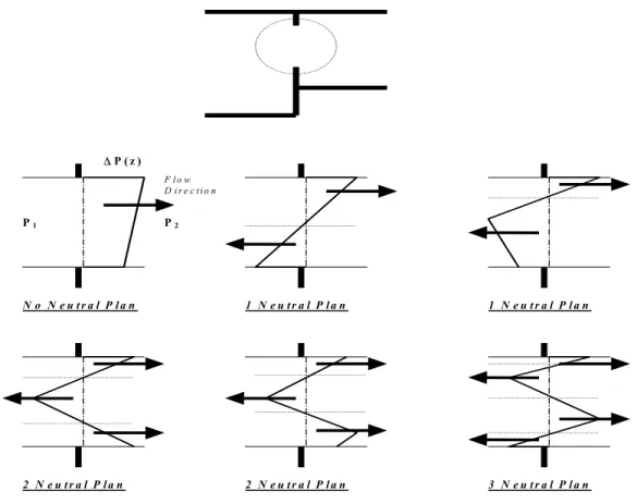
In order to divide a vent into several uni-directional parts, first we determine the positions of the neutral planes and flow directions, which can be estimated by calculating the pressure difference between the two sides of the vent.

Zi1 Zi2 U1 (upper layer) L1 (lower layer) U2 (upper layer) L2 (lower layer) Room 1 Room 2 Zf1 Zf2 Z Floor of room 1 Floor of room 2 Reference height Opening Zso Zsi

Figure 4.1 Basic vertical-vent (door/window) configuration

In Figure 4.1, Zi1 and Zi2 are the interface heights of the two compartments connected by a vent. Zso and Zsi are the soffit height and sill height of the vent with respect to the floor height of No.1 compartment, respectively. For each compartment, the pressure at the floor level is considered as the reference pressure. At any elevation Z, the pressures in the two compartments P1(Z) and P2(Z) can be obtained as follows:

{

1 1 1 1 1 1

}

1) min( , ) max[( ),0] ( 1 ) ( 1Z P Z_f g Z Z_f Zi _L Z Z_f Zi _U P = − − ρ + − − ρ (4.12)

{

2 2 2 2 2 2

}

2) min( , ) max[( ),0] ( 2 ) ( 2 Z P Z_f g Z Z_f Zi _L Z Z_f Zi _U P = − − ρ + − − ρ (4.13) ) ( 2 ) ( 1 ) (Z P Z P Z P = − ∆ (4.14)

where ∆P(Z) is the pressure difference between the two sides of the vent at height Z,

Zf1 and Zf2 are the floor elevations of the two compartments.

Z, Zf1 and Zf2 are defined with respect to the same reference height. The positions of the neutral planes are defined as the points where∆P(Z)=0. The number of neutral planes in an opening can range from zero to three (see Figure 4.2).

When hot smoke (U1) flows out of the vent, it may entrain air from the cool lower layer (L2) of the neighboring room and transport it into the upper layer. This process may be modeled by considering the vent flow as a plume induced by buoyancy. The virtual plume location can be estimated from inversely applying McCaffrey’s correlation. [3]

P1 P2 ∆P ( z ) F l o w D i r e c t i o n N o N e u t r a l P l a n 1 N e u t r a l P l a n 1 N e u t r a l P l a n 2 N e u t r a l P l a n 2 N e u t r a l P l a n 3 N e u t r a l P l a n

Figure 4.2 Possible neutral planes in an opening

2 1 2 1 ) ( _{U L U L} P C C T T m Q = − & ₋ (4.15) 08 . 0 011 . 0 0 . 0 , 011 . 0 566 . 0 / 1 2 1 566 . 0 / 1 2 1 5 / 2 ≤       <       = − − C L U C L U C V Q m if Q m Q Z & & (4.16) 20 . 0 026 . 0 08 . 0 , 026 . 0 909 . 0 / 1 2 1 909 . 0 / 1 2 1 5 / 2 ≤       <       = − − C L U C L U C V Q m if Q m Q Z & & (4.17) 895 . 1 / 1 2 1 895 . 1 / 1 2 1 5 / 2 124 . 0 20 . 0 , 124 . 0 _     <       = − − C L U C L U C V Q m if Q m Q Z & & (4.18) V e Z Z Z = ₁₂+ (4.19)

where QC is the equivalent convection heat release rate, 2

1 L

U

m& ₋ is the mass flow rate from layer U1 to layer L2,

ZV is the location of the virtual point plume,

Z12 is the real entrainment distance of the smoke flow given as follows:

[

]

[

]

2 ) ( ) ( , 0 max 2 ) ( ), ( max ) ( 1 2 2 1 1 1 2 2 12 f f f si f f Z Zso Z Zi Z Zi Z Zi Z Zi Z + − + + + + − + = (4.20)

Then from Ze and QC, plume entrainment rate from L2 to U2 can be calculated using Equations (4.1) to (4.4).

For Heskestad’s plume model, similar method can be used. The relevant equations are as follows: 5 / 2 0 0.166QC Z = (4.21) 1 0056 . 0 , 0056 . 0 2 1 2 1 0 ≤ = − − C L U C L U V Q m if Q m Z Z & & (4.22) 1 0056 . 0 , 071 . 0 0018 . 0 3/5 _{1 2} 3 / 1 2 1 >         ₋ = − − C L U C C L U V Q m if Q Q m Z & & (4.23) 26

Similarly, Ze and QC, plume entrainment rate from L2 to U2 can be calculated using Equations (4.5) to (4.7).

Additionally, when cool gas (L2) enters the neighboring zone (U1), it will behave like an inverse plume, and will entrain upper layer gas into the lower layer under some

conditions. In this model, the above equations are also used to calculate the inverse plume entrainment rate, and an equation similar to Equation (4.10) is used to limit the maximum plume entrainment rate.

4.3 Ceiling Vent Flow

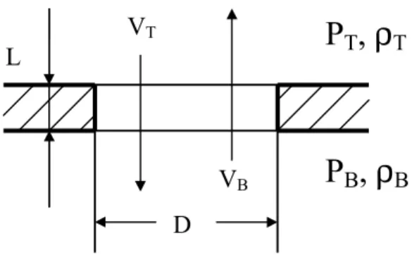
Vertical gas flow through a horizontal-vent involves two flow-driving mechanisms, buoyancy and pressure; while horizontal gas flow through a vertical-vent, such as a door, is considered to be driven only by pressure difference. It is not appropriate to directly use Bernoulli’s equation for ceiling vent flow because in addition to pressure difference, buoyant force has to be considered, which may lead to bi-directional flow. Cooper gives a calculation model for unstable flow through shallow, horizontal, circular vents under high-Grashof-number conditions, which is the case encountered in a building fire.[41-43] This has been included in this model as follows:

VB

VT

L

P

T

,

ρ

T

P

B

,

ρ

B

D

Figure 4.3 Basic horizontal-vent (ceiling vent) configuration

Let: ) , min( ), , max( _{T B L T B} H P P P P P P = = (4.24) 0 ≥ − = ∆P PH PL (4.25) 0 > − = ∆ρ ρT ρB (4.26) 27

2 / ) (ρ_B ρ_T ρ = + (4.27)    < ∆ − = ≥ ∆ = B T B T P P if P P if , / , / ρ ρ ε ρ ρ ε (4.28)

(

T_T T_B

)

2 T = + (4.29)

(

110.4

)

10 04128 . 0 × 7 2.5 + = − _{T T} ν (4.30) 2 3 2 ν ε gD Gr = (4.31)

where ν is the kinematic viscosity, and Gr is the Grashof number. If Gr is greater than 2 10× 7 then Cooper’s formulae can be used to calculate ceiling vent flow as follows. The following step is to judge whether it is under the condition of flooding or not; i.e., whether a bi-directional flow exists.

) 1072 . 1 exp( ) 2 / 1 ( 2427 . 0 +ε ε = Π_FL (4.32) FL FL g D P = ∆ Π ∆ (4 ρ ) (4.33) ) 5536 . 0 exp( 1754 . 0 ,FL = ε H Fr (4.34) FL H V FL H gD A Fr V _, =(2 ε)1/2 _, (4.35)

If , then unidirectional flow is expected, and the relevant calculation formulae are as follows: FL P P≥∆ ∆

[

]

{

FL

}

HFL H p p V V = 1.19252+11.3569(∆ /∆ −1) 1/2 −0.092025 _, (4.36) 0 = L V (4.37) H N V V = (4.38)

where V is the volume flow rate through the vent,

subscripts H, L and N refer to flow from the high pressure side to the low pressure side, from the low to the high side and the net flow rate.

If , then bi-directional exchange flow will exist, and the relevant calculation formulas are as follows:

FL P P<∆ ∆ 2 / 1 , 0.055(4/π)A (gDε) V_EXMAX = _V (4.39)

[

]

FL H FL N V P P V _, 2 / 1 4 . 8 ) / 1 ( 36 . 87 1 4 . 9 − + −∆ ∆ = (4.40)

[

FL FL

]

EXMAX L P P P P V V = 0.6465(1−∆ /∆ )2 −1.6465(1−∆ /∆ ) 2 _, (4.41) N L H V V V = + (4.42)

In this model, if the condition using the above Cooper’s model is not satisfied, then the uni-directional Bernoulli’s equation is directly used as follows:

H V CV H P A C V ρ ∆ = 2 (4.43)

where CCV is the coefficient of ceiling vent flow, which is taken as 0.61 in this model.

4.4 Mechanical Ventilation

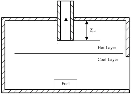
Mechanical ventilation is considered using a specification model. Figure 4.4 shows a schematic of a mechanical ventilation opening. Through the opening, smoke can be extracted out of the room to ambient, or ambient air can be supplied into the room. Two parameters can be specified in this model. One is the Zext, the vertical extension of the

opening away from the ceiling surface, another is the mechanical volume or mass ventilation rate.

In the case shown in Figure 4.4, initially the smoke interface is above the opening elevation, and the exhausted gas is lower layer air only. If the plume entrainment rate at the elevation of the exhaust opening is greater than the exhaust rate, then the interface will be formed under the opening, and after that time, the exhausted gas will be smoke only. If the plume entrainment rate at the elevation of the exhaust opening is less than the exhaust rate, and the smoke exhaust system is assumed to be ideally effective, then the interface will be formed at the opening elevation, and the exhausted gas is assumed to be composed of two parts, smoke and lower layer gas. For this case, the following

formulation has been used in the model to identify how much gas is extracted from each zone.

For mass flow rate specification:

) , min(m m_max

m&_MU = &_Fan & (4.44)

MU Fan

ML m m

m& = & − & (4.45)

For Volume flow rate specification:

) , min( max U Fan MU m V V ρ & & & _{= (4.46)} MU Fan ML V V

V& = & − & (4.47)

where is the maximum smoke exhaust rate from the upper layer. and m are mass flow rate exhausted from upper layer and lower layer, respectively. m is the specified mass exhaust rate of the exhaust fan. V and V are volume flow rate exhausted from upper layer and lower layer, respectively. V is the specified volume exhaust rate of the exhaust fan.

max m& m&_MU & ML & Fan MU & ML & & Fan

The above method of limiting the maximum smoke exhaust rate is also helpful in ensuring the numerical stability and efficiency, when the exhausted gas is composed of two parts, smoke and the lower layer gas. Sometimes is difficult to calculate. For the situation shown in Figure 4.4, where a ceiling vent is not provided and the soffit of the door is lower than the opening, is the plume entrainment rate at the elevation of the opening. max m& max m& Zext Cool Layer Hot Layer Fuel

Figure 4.4 Schematic of the mechanical ventilation opening

4.5 Stair Shaft Flow

When dealing with multi-storey buildings, it is important to compute the mass or volume flow rate through a stair shaft, because a stair shaft is the main path of smoke spread from floor to floor. Achakji and Tamura conducted research work on pressure drop

characteristics of typical stairshafts in high-rise buildings [44]. It was found that pressure drop through a stairshaft can be represented by a pressure loss across an equivalent horizontal orifice located between floors of a frictionless stair shaft.

Based on Achakji and Tamura’s experimental data, a correlation for calculating the area of the effective orifice was obtained and used in CONTAM, a model used to analyze contaminant migration in a building [45]. This correlation is as follows:

For open treads:

) 14 . 0 0 . 1 ( 089 . 0 _{i S i} i h A d Ae = − (4.48)

For closed treads:

) 24 . 0 0 . 1 ( 083 . 0 _{i S i} i h A d Ae = − (4.49)

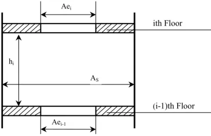
As shown in Figure 4.5, the parameters in the above two equations are as follows: is the effective orifice area on the ith floor, is the height of the shaft between the ith floor and (i-1)th floor, is the density of people on the stairs between the ith floor and (i-1)th floor, and is the cross-sectional area of the stair shaft.

i Ae i h i d S A (i-1)th Floor hi AS ith Floor Aei Aei-1

Figure 4.5 Schematic of an effective ceiling vent for a stair shaft

Equations (4.48) and (4.49) were used in previous version of FIERAsmoke. However, it was found that there is a problem in the two equations with the relationship between and . Following equations (4.48) and (4.49), the higher is, the larger the area is. This is contradictory to the real physical laws of fluid flow. As h represents the length of friction in the stairshaft, it is expected that increasing will increase friction and decrease the effective area . After carefully re-investigating the original paper

i Ae i i h h_i i Ae i h i Ae [44]

referenced by CONTAM, it was found that the following equation is given:

2 1 1       = e i CV S i D h k C A Ae (4.50)

where C_CV is the coefficient of discharge as in section 4.3, taken as 0.6 in reference [44]; k is the friction pressure loss coefficient; is equivalent diameter, which can be

calculated by the stairshaft cross-sectional area and the perimeter of the shaft

e D S A Γ as follows: Γ = S e A D 4 (4.51)

Equation (4.50), however does not include the effect of the density of people . To account for this, the approach used in Equations (4.48) and (4.49) is followed, resulting in the following equation that is used in the model:

i d 2 1 ) 0 . 1 (       − = e i CV i S i D h k C d A Ae β (4.52)

where, β is taken as 0.14 for open tread case, 0.24 for closed tread case. According to reference,[44] k is taken as 29 for open tread case and 32 for closed tread case. In the model, after the equivalent area Ae_i is obtained from Equation (4.52), Cooper’s [43] ceiling vent flow model is used to calculate the volumetric flow rate through the ceiling vent, as mentioned in section 4.3.

4.6 Species Concentration

Suppose at time t in a well-stirred gas layer, there are NS kinds of species, the total mass is m, and the mass fraction of species K is YK, K=1, 2, …, NS.

Then, at the next time step t+∆t, the concentration of the Kth species will be approximated as follows:

[

]

[

∑

∑

+

∑

∑

]

∆ + + ∆ + = ∆ + V e K V K e K t t K m m t m m m t mY Y & & & & _{, ,} ) ( , K=1, 2, …, NS. (4.53)

where and are the total net mass flow rate entering the layer (negative for flowing out) by plume entrainment and vent flow.

∑

m&e

∑

m&V

∑

m&e,K and

∑

are the total net

mass flow rate of species K entering the layer by plume and vent flow.

K V

m& _,

5. HEAT TRANSFER

5.1 Conduction Heat Transfer

To calculate conduction heat transfer through the compartment boundaries, a one-dimensional conduction model is used. The governing equation is as follows:

0 , 0 , 2 2 ≥ ≤ ≤ ∂ ∂ = ∂ ∂ t L x x T C K t T ρ (5.1)

Due to the complexity of the building geometry, it is assumed that heat is transferred to the outside and not to the gas of the neighboring rooms as in CFAST. Then the following initial and boundary conditions can be given:

) 0 , ( , 0 , 0≤x≤L t = T =T x (5.2) IR g IC T T t q h x T k x = − + ∂ ∂ − =0, ( (0, )) (5.3) OR a OC T T L t q h x T k L x =− − − ∂ ∂ − = , ( ( , )) (5.4)

where hIC and hOC are heat transfer coefficients of the inside and outside surface of the wall, and and are the net radiation heat fluxes from gas received by inside and outside surfaces of the wall. The T(x, 0) is the temperature profile at the initial time, from which we can predict the temperature profile at any future time by coupling conduction with convection and radiation.

IR

q q_OR

5.2 Convection Heat Transfer in Non-Fire Rooms

Convection heat transfer in a non-fire room may be considered to be a natural convection system. The following equations for turbulent convection heat transfer are included in this model:[3, 46, 47] w conv conv q A Q = (5.5) 34

where Q and are the convection heat loss and flux to a surface of a wall, ceiling or floor, and A

conv qconv

w is the heat transfer area, )

( _{g w}

conv h T T

q = − (5.6)

where Tg is the temperature of gas, and Tw is the temperature of the surface of a wall, ceiling or floor. h is the convection heat transfer coefficient given as follows:

Nu l K

h= (5.7)

K is the gas conductivity, l is the characteristic length, and Nu is the Nusselt number. l, K and Nu numbers can be obtained as below:

w A l= (5.8)

( )

0.8 4 10 72 . 2 T K = × − (5.9)

(

)

1/3 Pr Gr C Nu= _conv (5.10)

where Cconv is a constant. For a wall Cconv=0.13, for a heated floor or a cooled ceiling

Cconv=0.021, for a cooled floor or a heated ceiling Cconv=0.21. T is the averaged

temperature as follows: 2 w g T T T = +

In Equation (5.10), Pr is the Prandtl number of air, which is taken as a constant 0.7. Gr is the Grashof number:

2 3 ν T T gl Gr = ∆ (5.11) where w g T T T = − ∆ (5.12)

And ν is the kinematic viscosity calculated using Equation (4.30).