A Generalized Markov-Chain Modelling Approach to (1,λ)-ES Linear Optimization

HAL Id: hal-01091494

https://hal.inria.fr/hal-01091494

Submitted on 5 Dec 2014

HAL is a multi-disciplinary open access

archive for the deposit and dissemination of

sci-entific research documents, whether they are

pub-lished or not. The documents may come from

teaching and research institutions in France or

abroad, or from public or private research centers.

L’archive ouverte pluridisciplinaire HAL, est

destinée au dépôt et à la diffusion de documents

scientifiques de niveau recherche, publiés ou non,

émanant des établissements d’enseignement et de

recherche français ou étrangers, des laboratoires

publics ou privés.

A Generalized Markov-Chain Modelling Approach to

(1,λ)-ES Linear Optimization

Alexandre Chotard, Martin Holeňa

To cite this version:

Alexandre Chotard, Martin Holeňa. A Generalized Markov-Chain Modelling Approach to (1,λ)-ES

Linear Optimization. Parallel Problem Solving from Nature – PPSN XIII, Sep 2014, Ljubljana,

Slovenia. pp.902 - 911, �10.1007/978-3-319-10762-2_89�. �hal-01091494�

A Generalized Markov-Chain Modelling

Approach to (1, λ)-ES Linear Optimization

Alexandre Chotard1_{and Martin Holeˇna}2

1 _{INRIA Saclay-Ile-de-France, LRI, [email protected] University}

Paris-Sud, France

2 _{Institute of Computer Science, Academy of Sciences, Pod vod´arenskou vˇeˇz´ı 2,}

Prague, Czech Republic, [email protected]

Abstract. Several recent publications investigated Markov-chain mod-elling of linear optimization by a (1, λ)-ES, considering both uncon-strained and linearly conuncon-strained optimization, and both constant and varying step size. All of them assume normality of the involved random steps, and while this is consistent with a black-box scenario, information on the function to be optimized (e.g. separability) may be exploited by the use of another distribution. The objective of our contribution is to complement previous studies realized with normal steps, and to give suf-ficient conditions on the distribution of the random steps for the success of a constant step-size (1, λ)-ES on the simple problem of a linear func-tion with a linear constraint. The decomposifunc-tion of a multidimensional distribution into its marginals and the copula combining them is applied to the new distributional assumptions, particular attention being paid to distributions with Archimedean copulas.

Keywords: evolution strategies, continuous optimization, linear opti-mization, linear constraint, linear function, Markov chain models, Archimedean copulas

1

Introduction

Evolution Strategies (ES) are Derivative Free Optimization (DFO) methods, and as such are suited for the optimization of numerical problems in a black-box context, where the algorithm has no information on the function f it optimizes (e.g. existence of gradient) and can only query the function’s values. In such a context, it is natural to assume normality of the random steps, as the normal distribution has maximum entropy for given mean and variance, meaning that it is the most general assumption one can make without the use of additional information on f . However such additional information may be available, and then using normal steps may not be optimal. Cases where different distributions have been studied include so-called Fast Evolution Strategies [1] or SNES [2, 3] which exploits the separability of f , or heavy-tail distributions on multimodal problems [4, 3].

In several recent publications [5–8], attention has been paid to Markov-chain modelling of linear optimization by a (1, λ)-ES, i.e. by an evolution strategy in

which λ children are generated from a single parent X ∈ Rn _{by adding normally}

distributed n-dimensional random steps M ,

X_{← X + σC}

1

2M_{, where M ∼ N (0, I}n). (1)

Here, σ is called step size, C is a covariance matrix, and N (0, In) denotes the

n-dimensional standard normal distribution with zero mean and covariance matrix identity. The best among the λ children, i.e. the one with the highest fitness, becomes the parent of the next generation, and the step-size σ and the covariance matrix C may then be adapted to increase the probability of sampling better children. In this paper we relax the normality assumption of the movement M to a more general distribution H.

The linear function models a situation where the step-size is relatively small compared to the distance towards a local optimum. This is a simple problem that must be solved by any effective evolution strategy by diverging with positive increments of ∇f.M . This unconstrained case was studied in [7] for normal steps with cumulative step-size adaptation (the step-size adaptation mechanism in CMA-ES [9]).

Linear constraints naturally arise in real-world problems (e.g. need for posi-tive values, box constraints) and also model a step-size relaposi-tively small compared to the curvature of the constraint. Many techniques to handle constraints in ran-domised algorithms have been proposed (see [10]). In this paper we focus on the resampling method, which consists in resampling any unfeasible candidate until a feasible one is sampled. We chose this method as it makes the algorithm eas-ier to study, and is consistent with the previous studies assuming normal steps [11, 5, 6, 8], studying constant step-size, self adaptation and cumulative step-size adaptation mechanisms (with fixed covariance matrix).

Our aim is to study the (1, λ)-ES with constant step-size, constant covari-ance matrix and random steps with a general absolutely continuous distribution H optimizing a linear function under a linear constraint handled through re-sampling. We want to extend the results obtained in [5, 8] using the theory of Markov chains. It is our hope that such results will help in designing new algo-rithms using information on the objective function to make non-normal steps. We pay a special attention to distributions with Archimedean copulas, which are a particularly well transparent alternative to the normal distribution. Such distributions have been recently considered in the Estimation of Distribution Algorithms [12, 13], continuing the trend of using copulas in that kind of evolu-tionary optimization algorithms [14].

In the next section, the basic setting for modelling the considered evolu-tionary optimization task is formally defined. In Section 3, the distributions of the feasible steps and of the selected steps are linked to the distribution of the random steps, and another way to sample them is provided. In Section 4, it is shown that, under some conditions on the distribution of the random steps, the normalized distance to the constraint defined in (5) is a ergodic Markov chain, and a law of large numbers for Markov chains is applied. Finally, Section 5 gives properties on the distribution of the random steps under which some of the aforementioned conditions are verified.

Due to a lack of space proofs were not included in this paper, and can instead be found at http://hal.inria.fr/docs/01/00/30/15/PDF/ppsn2014TRlinear constraintgeneraldistributions.pdf.

Notations

For (a, b) ∈ N2_{with a < b, [a..b] denotes the set of integers i such that a ≤ i ≤ b.}

For X and Y two random vectors, X (d)= Y denotes that these variables are equal in distribution, X a.s.→ Y and X → Y denote, respectively, almost sureP convergence and convergence in probability. For (x, y) ∈ Rn_{, x.y denotes the}

scalar product between the vectors x and y, and for i ∈ [1..n], [x]i denotes the

ith _{coordinate of x. For A a subset of R}n_,

1A denotes the indicator function of A. For X a topological set, B(X ) denotes the Borel algebra on X .

2

Problem setting and algorithm definition

Throughout this paper, we study a (1, λ)-ES optimizing a linear function f : Rn → R where λ ≥ 2 and n ≥ 2, with a linear constraint g : Rn _{→ R,}

han-dling the constraint by resampling unfeasible solutions until a feasible solution is sampled.

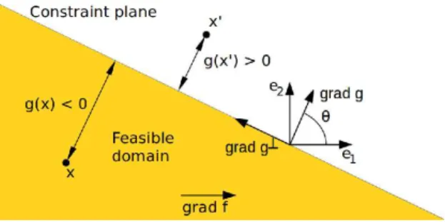
Take (ek)k∈[1..n] a orthonormal basis of Rn. We may assume ∇f to be

nor-malized as the behaviour of an ES is invariant to the composition of the objective function by a strictly increasing function (e.g. h : x 7→ x/k∇f k), and the same holds for ∇g since our constraint handling method depends only on the inequality g(x) ≤ 0 which is invariant to the composition of g by a homothetic transforma-tion. Hence w.l.o.g. we assume that ∇f = e1 and ∇g = cos θe1+ sin θe2 with

the set of feasible solutions Xfeasible:= {x ∈ Rn|g(x) ≤ 0}. We restrict our study

to θ ∈ (0, π/2). Overall the problem reads

maximize f (x) = [x]1 subject to

g(x) = [x]1cos θ + [x]2sin θ ≤ 0 .

(2) At iteration t ∈ N, from a so-called parent point Xt ∈ Xfeasible and with

step-size σt∈ R∗+ we sample new candidate solutions by adding to Xta random

vector σtMi,jt where M i,j

t is called a random step and (M i,j

t )i∈[1..λ],j∈N,t∈N is

a i.i.d. sequence of random vectors with distribution H. The i index stands for the λ new samples to be generated, and the j index stands for the unbounded number of samples used by the resampling. We denote Mit a feasible step, that

is the first element of (Mi,jt )j∈N such that Xt+ σtMit∈ Xfeasible(random steps

are sampled until a suitable candidate is found). The ith _{feasible solution Y}i tis

then

Yi_t:= Xt+ σtMit . (3)

Then we denote ⋆ := argmaxi∈[1..λ]f (Yit) the index of the feasible solution

maximizing the function f , and update the parent point

Fig. 1.Linear function with a linear constraint, in the plane spanned by ∇f and ∇g, with the angle from ∇f to ∇g equal to θ ∈ (0, π/2). The point x is at distance g(x) from the constraint hyperplan g(x) = 0.

where M⋆t is called the selected step. Then the step-size σt, the distribution of

the random steps H or other internal parameters may be adapted. Following [5, 6, 11, 8] we define δtas

δt:= −

g(Xt)

σt

. (5)

3

Distribution of the feasible and selected steps

In this section we link the distributions of the random vectors Mit and M⋆t to

the distribution of the random steps Mi,jt , and give another way to sample Mit

and M⋆t not requiring an unbounded number of samples.

Lemma 1. Let a (1, λ)-ES optimize the problem defined in (2) handling con-straint through resampling. Take H the distribution of the random step Mi,jt ,

and for δ ∈ R∗

+ denote Lδ := {x ∈ Rn|g(x) ≤ δ}. Providing that H is absolutely

continuous and that H(Lδ) > 0 for all δ ∈ R+, the distribution ˜Hδ of the

feasi-ble step and ˜H⋆

δ the distribution of the selected step when δt= δ are absolutely

continuous, and denoting h, ˜hδ and ˜h⋆δ the probability density functions of,

re-spectively, the random step, the feasible step Mit and the selected step M ⋆ t when δt= δ ˜ hδ(x) = h(x)1L δ(x) H(Lδ) , (6) and ˜ h⋆δ(x) = λ˜hδ(x) ˜Hδ((−∞, [x]1) × Rn−1)λ−1 = λh(x)1L δ(x)H((−∞, [x]1) × R n−1_{∩ L} δ)λ−1 H(Lδ)λ . (7)

The vectors (Mit)i∈[1..λ]and M⋆tare functions of the vectors (M i,j

t )i∈[1..λ],j∈N

is given which uses a finite number of samples. This method is useful if one wants to avoid dealing with the infinite dimension space implied by the sequence (Mi,jt )i∈[1..λ,j∈N.

Lemma 2. Let a (1, λ)-ES optimize problem (2), handling the constraint through resampling, and take δtas defined in (5). Let H denote the distribution of Mi,jt

that we assume absolutely continuous, ∇g⊥ _{:= − sin θe}

1+ cos θe2, Q the

ro-tation matrix of angle θ changing (e1, e2, . . . , en) into (∇g, ∇g⊥, . . . , en). Take

F1,δ(x) := Pr(Mit.∇g ≤ x|δt = δ), F2,δ(x) := Pr(Mit.∇g⊥ ≤ x|δt = δ) and

Fk,δ(x) := Pr([Mit]k≤ x|δt= δ) for k ∈ [3..n], the marginal cumulative

distribu-tion funcdistribu-tions when δt= δ, and Cδ the copula of (Mit.∇g, Mti.∇g⊥, . . . , Mit.en).

We define G : (δ, (ui)i∈[1..n]) ∈ R+× [0, 1]n7→ Q    F_1,δ−1(u1) .. . F_n,δ−1(un)    , (8) G⋆ : (δ, (vi)i∈[1..λ]) ∈ R+× [0, 1]nλ 7→ argmax G∈{G(δ,vi)|i∈[1..λ]} f (G) . (9) Then, if the copula Cδ is constant in regard to δ, for Wt= (Vi,t)i∈[1..λ] a i.i.d.

sequence with Vi,t ∼ Cδ

G(δt, Vi,t) (d) = Mit , (10) G⋆_(δ t, Wt) (d) = M⋆t . (11)

We may now use these results to show the divergence of the algorithm when the step-size is constant, using the theory of Markov chains [15].

4

Divergence of the (1, λ)-ES with constant step-size

Following the first part of [8], we restrict our attention to the constant step size in the remainder of the paper, that is for all t ∈ N we take σt= σ ∈ R∗+.

From Eq. (4), by recurrence and dividing by t, we see that [Xt− X0]1 t = σ t t−1 X i=0 M⋆_i . (12)

The latter term suggests the use of a Law of Large Numbers to show the con-vergence of the left hand side to a constant that we call the dicon-vergence rate. The random vectors (M⋆t)t∈Nare not i.i.d. so in order to apply a Law of Large

Num-bers on the right hand side of the previous equation we use Markov chain theory, more precisely the fact that (M⋆t)t∈Nis a function of a (δt, (Mi,jt )i∈[1..λ],j∈N)t∈N

which is a geometrically ergodic Markov chain. As (Mi,jt )i∈[1..λ],j∈N,t∈Nis a i.i.d.

sequence, it is a Markov chain, and the sequence (δt)t∈N is also a Markov chain

Proposition 1. Let a (1, λ)-ES with constant step-size optimize problem (2), handling the constraint through resampling, and take δtas defined in (5). Then

no matter what distribution the i.i.d. sequence (Mi,jt )i∈[1..λ],(j,t)∈N2have, (δ_t)_t∈N

is a homogeneous Markov chain and

δt+1= δt− g(M⋆t) = δt− cos θ[M⋆t]1− sin θ[M⋆t]2 . (13)

We now show ergodicity of the Markov chain (δt)t∈N, which implies that the

t-steps transition kernel (the function A 7→ Pr(δt ∈ A|δ0 = δ) for A ∈ B(R+))

converges towards a stationary measure π, generalizing Propositions 3 and 4 of [8].

Proposition 2. Let a (1, λ)-ES with constant step-size optimize problem (2), handling the constraint through resampling. We assume that the distribution of Mi,jt is absolutely continuous with probability density function h, and that h

is continuous and strictly positive on Rn_{. Denote µ}

+ the Lebesgue measure on

(R+, B(R+)), and for α > 0 take the functions V : δ 7→ δ, Vα: δ 7→ exp(αδ) and

r1: δ 7→ 1. Then (δt)t∈N is µ+-irreducible, aperiodic and compact sets are small

sets for the Markov chain.

If the following two additional conditions are fulfilled

E(|g(Mi,jt )| | δt= δ) < ∞ for all δ ∈ R+ , and (14)

lim

δ→+∞E(g(M ⋆

t)|δt= δ) ∈ R∗+ , (15)

then (δt)t∈Nis r1-ergodic and positive Harris recurrent with some invariant

mea-sure π.

Furthermore, if

E(exp(g(Mi,jt ))|δt= δ) < ∞ for all δ ∈ R+ , (16)

then for α > 0 small enough, (δt)t∈N is also Vα−geometrically ergodic.

We now use a law of large numbers ([15] Theorem 17.0.1) on the Markov chain (δt, (Mi,jt )i∈[1..λ],j∈N)t∈N to obtain an almost sure divergence of the algorithm.

Proposition 3. Let a (1, λ)-ES optimize problem (2), handling the constraint through resampling. Assume that the distribution H of the random step Mi,jt is

absolutely continuous with continuous and strictly positive density h, that condi-tions (16) and (15) of Proposition 2 hold, and denote π and µM the stationary

distribution of respectively (δt)t∈N and (Mi,jt )i∈[1..λ],(j,t)∈N2. Then

[Xt− X0]1 t a.s. −→ t→+∞σEπ×µM([M ⋆ t]1) . (17)

Furthermore if E([M⋆t]2) < 0, then the right hand side of Eq. (17) is strictly

5

Application to More Specific Distributions

Throughout this section we give cases where the assumptions on the distribution of the random steps H used in Proposition 2 or Proposition 3 are verified.

The following lemma shows an equivalence between a non-identity covariance matrix for H and a different norm and constraint angle θ.

Lemma 3. Let a (1, λ)-ES optimize problem (2), handling the constraint with resampling. Assume that the distribution H of the random step Mi,jt has

pos-itive definite covariance matrix C with eigenvalues (α2

i)i∈[1..n] and take B =

(bi,j)(i,j)∈[1..n]2 such that BCB−1 is diagonal. Denote A_H,g,X0 the sequence of

parent points (Xt)t∈N of the algorithm with distribution H for the random steps

Mi,j_t , constraint angle θ and initial parent X0. Then for all k ∈ [1..n]

βk[AH,θ,X0]_k (d) =hAC−1/2H,θ′,X′ 0 i k , (18) where βk = r Pn j=1 b2 j,i α2 i , θ ′ _{= arccos(}β1cosθ βg ) with βg = q β2 1cos2θ + β22sin2θ,

and [X′0]k= βk[X0]k for all k ∈ [1..n].

Although Eq. (17) shows divergence of the algorithm, it is important that it diverges in the right direction, i.e. that the right hand side of Eq. (17) has a positive sign. This is achieved when the distribution of the random steps is isotropic, as stated in the following proposition.

Proposition 4. Let a (1, λ)-ES optimize problem (2) with constant step-size, handling the constraint with resampling. Suppose that the Markov chain (δt)t∈N

is positive Harris, that the distribution H of the random step Mi,j_t is absolutely continuous with strictly positive density h, and take C its covariance matrix. If the distribution C−1/2_{H is isotropic then E}

π×µM([M

⋆ t]1) > 0.

Lemma 3 and Proposition 4 imply the following result to hold for multivariate normal distributions.

Proposition 5. Let a (1, λ)-ES optimize problem (2) with constant step-size, handling the constraint with resampling. If H is a multivariate normal distribu-tion with mean 0, then (δt)t∈N is a geometrically ergodic positive Harris Markov

chain, Eq. (17) holds and its right hand side is strictly positive.

To obtain sufficient conditions for the density of the random steps to be strictly positive, it is advantageous to decompose that distribution into its marginals and the copula combining them. We pay a particular attention to Archimedean copulas, i.e., copulas defined

(∀u ∈ [0, 1]n_{) C}

where ψ : [0, +∞] → [0, 1] is an Archimedean generator, i.e., ψ(0) = 1, ψ(+∞) = limt→+∞ψ(t) = 0, ψ is continuous and strictly decreasing on [0, inf{t : ψ(t) =

0}), and ψ−1 _{denotes the generalized inverse of ψ,}

(∀u ∈ [0, 1]) ψ−1_{(u) = inf{t ∈ [0, +∞] : ψ(t) = u}. (20)}

The reason for our interest is that Archimedean copulas are invariant with re-spect to permutations of variables, i.e.,

(∀u ∈ [0, 1]n) Cψ(Qu) = Cψ(u). (21)

holds for any permutation matrix Q ∈ Rn,n_{. This can be seen as a weak form of}

isotropy because in the case of isotropy, (19) holds for any rotation matrix, and a permutation matrix is a specific rotation matrix.

Proposition 6. Let H be the distribution of the two first dimensions of the random step Mi,jt , H1 and H2 be its marginals, and C be the copula relating H

to H1 and H2. Then the following holds:

1. Sufficient for H to have a continuous strictly positive density is the simul-taneous validity of the following two conditions.

(i) H1and H2have continuous strictly positive densities h1 and h2,

respec-tively.

(ii) C has a continuous strictly positive density c. Moreover, if (i) and (ii) are valid, then

(∀x ∈ R2) h(x) = c(H1([x]1), H2([x]2))h1([x]1)h2([x]2). (22)

2. If C is Archimedean with generator ψ, then it is sufficient to replace (ii) with (ii’) ψ is at least 4-monotone, i.e., ψ is continuous on [0, +∞], ψ′′_is

decreas-ing and convex on R+, and (∀t ∈ R+) (−1)kψ(k)(t) ≥ 0, k = 0, 1, 2.

In this case, if (i) and (ii’) are valid, then

(∀x ∈ R2) h(x) = ψ ′′_(ψ−1_(H 1([x]1)) + ψ−1(H2([x]2))) ψ′_(ψ−1_(H 1([x]1)) + ψ−1(H2([x]2)))h1([x]1)h2([x]2). (23)

6

Discussion

The paper presents a generalization of recent results of the first author [8] con-cerning linear optimization by a (1, λ)-ES in the constant step size case. The generalization consists in replacing the assumption of normality of random steps involved in the evolution strategy by substantially more general distributional assumptions. This generalization shows that isotropic distributions solve the linear problem. Also, although the conditions for the ergodicity of the studied Markov chain accept some heavy-tail distributions, an exponentially vanishing tail allow for geometric ergodicity, which imply a faster convergence to its sta-tionary distribution, and faster convergence of Monte Carlo simulations. In our

opinion, these conditions increase the insight into the role that different kinds of distributions play in evolutionary computation, and enlarges the spectrum of possibilities for designing evolutionary algorithms with solid theoretical funda-mentals. At the same time, applying the decomposition of a multidimensional distribution into its marginals and the copula combining them, the paper at-tempts to bring a small contribution to the research into applicability of copulas in evolutionary computation, complementing the more common application of copulas to the Estimation of Distribution Algorithms [12, 14, 13].

Needless to say, more realistic than the constant step size case, but also more difficult to investigate, is the varying step size case. The most important results in [8] actually concern that case. A generalization of those results for non-Gaussian distributions of random steps for cumulative step-size adaptation ([9]) is especially difficult as the evolution path is tailored for Gaussian steps, and some careful tweaking would have to be applied. The σ self-adaptation evolution strategy ([16]), studied in [6] for the same problem, appears easier, and would be our direction for future research.

Acknowledgment

The research reported in this paper has been supported by grant ANR-2010-COSI-002 (SIMINOLE) of the French National Research Agency, and Czech Science Foundation (GA ˇCR) grant 13-17187S.

References

1. X. Yao and Y. Liu, “Fast evolution strategies,” in Evolutionary Programming VI, pp. 149–161, Springer, 1997.

2. T. Schaul, “Benchmarking Separable Natural Evolution Strategies on the Noiseless and Noisy Black-box Optimization Testbeds,” in Black-box Optimization

Bench-marking Workshop, Genetic and Evolutionary Computation Conference,

(Philadel-phia, PA), 2012.

3. T. Schaul, T. Glasmachers, and J. Schmidhuber, “High dimensions and heavy tails for natural evolution strategies,” in Genetic and Evolutionary Computation

Conference (GECCO), 2011.

4. N. Hansen, F. Gemperle, A. Auger, and P. Koumoutsakos, “When do heavy-tail distributions help?,” in Parallel Problem Solving from Nature PPSN IX (T. P. Runarsson et al., eds.), vol. 4193 of Lecture Notes in Computer Science, pp. 62–71, Springer, 2006.

5. D. Arnold, “On the behaviour of the (1,λ)-ES for a simple constrained problem,” in Foundations of Genetic Algorithms - FOGA 11, pp. 15–24, ACM, 2011. 6. D. Arnold, “On the behaviour of the (1, λ)-σSA-ES for a constrained linear

prob-lem,” in Parallel Problem Solving from Nature - PPSN XII, pp. 82–91, Springer, 2012.

7. A. Chotard, A. Auger, and N. Hansen, “Cumulative step-size adaptation on lin-ear functions,” in Parallel Problem Solving from Nature - PPSN XII, pp. 72–81, Springer, september 2012.

8. A. Chotard, A. Auger, and N. Hansen, “Markov chain analysis of evolution strate-gies on a linear constraint optimization problem,” in 2014 IEEE Congress on

Evo-lutionary Computation (CEC).

9. N. Hansen and A. Ostermeier, “Completely derandomized self-adaptation in evo-lution strategies,” Evoevo-lutionary Computation, vol. 9, no. 2, pp. 159–195, 2001. 10. C. A. Coello Coello, “Constraint-handling techniques used with evolutionary

al-gorithms,” in Proceedings of the 2008 GECCO conference companion on Genetic

and evolutionary computation, GECCO ’08, (New York, NY, USA), pp. 2445–2466,

ACM, 2008.

11. D. Arnold and D. Brauer, “On the behaviour of the (1 + 1)-ES for a simple con-strained problem,” in Parallel Problem Solving from Nature - PPSN X (I. G. R. et al., ed.), pp. 1–10, Springer, 2008.

12. A. Cuesta-Infante, R. Santana, J. Hidalgo, C. Bielza, and P. Larra˜naga, “Bivariate empirical and n-variate archimedean copulas in estimation of distribution algo-rithms,” in IEEE Congress on Evolutionary Computation, pp. 1–8, 2010.

13. L. Wang, X. Guo, J. Zeng, and Y. Hong, “Copula estimation of distribution al-gorithms based on exchangeable archimedean copula,” International Journal of

Computer Applications in Technology, vol. 43, pp. 13–20, 2012.

14. R. Salinas-Gutierrez, A. Hern´andez Aguirre, and E. Villa Diharce, “Using copulas in estimation of distribution algorithms,” in MICAI 2009: Advances in Artificial

Intelligence, pp. 658–668, 2009.

15. S. P. Meyn and R. L. Tweedie, Markov chains and stochastic stability. Cambridge University Press, second ed., 1993.

16. H.-G. Beyer, “Toward a theory of evolution strategies: Self-adaptation,”