A central composite design to investigate antibody fragment production by Pichia pastoris

A Central Composite Design to Investigate Antibody

Fragment Production by Pichia pastoris

by

Joyce Chan

Submitted to the Biological Engineering Division

in partial fulfillment of the requirements for the degree of Master of Engineering in Biomedical Engineering

at the

MASSACHUSETTS INSTITUTE OF TECHNOLOGY

September 2005

© Massachusetts Institute of Technology 2005. All rights reserved.

Author

...

-

Biological Engineering Division

August 5, 2005

Certified

by...

_{... /..//...-//~.-. ...}

MASSACHUSE7TS INSl E

OFTECHNOLOGY

LBOCT 2AR 2005ES

LIBRARI ES i

A Central Composite Design to Investigate Antibody

Fragment Production by Pichia pastoris

by

Joyce Chan

Submitted to the Biological Engineering Division on August 5, 2005, in partial fulfillment of the

requirements for the degree of

Master of Engineering in Biomedical Engineering

Abstract

This study aims to investigate the relationships between growth parameters (agita-tion, glycerol concentra(agita-tion, salt concentration) and responses (biomass, growth rate, protein expression), by a 3-factor-3-level central composite factorial design. This ex-perimental design involved running shake flask culture at 15 different explerimental conditions with duplicates. Optical density (OD600), dry cell weight (DCXV), and BCA Protein Assays were done on each experiment. Mathematical models in terms of these parameters' effects and their interactions were proposed for each of the re-sponses. The significance of each effect and interaction, as well as the goodness-of-fit of mathematical models to data were examined by analysis of variance. It was found that biomass (with RAdj-0.951) is a strong function of glycerol concentration (higher glycerol concentration leads to higher biomass), but it varies much less with agitation, and it is completely independent of salt concentration. Growth rate (RAd=--0.901), however, varies strongly with agitation and salt concentration, but much more weakly with glycerol concentration. Protein production has a low RAdj value of ().746, imn-plying that higher-order terms, e.g. x2 and x2, should be tested for significance in the model. Collected data were fitted to the proposed models by response surface regression, after which surface and contour plots of responses were generated to iden-tify trends in them. High agitation (300 rpm in shaker) gave rise to both highest biomass and growth rate. In addition, biomass at high glycerol concentration (3% v/v) was almost twice as much as biomass at low glycerol concentration (1% v/v) at high agitation rate (19 g/L compared to 11 g/L). At the same agitation rate, growth rate shows the largest increase of 20.5% with increasing salt concentration from 0.7% to 2.1%. Protein production reached maximum of 7.3 mg/mL at medium agitation rate (250 rpm), high salt and glycerol concentrations.

Thesis Supervisor: Jean-Francois Hamel Title: Lecturer

Acknowledgments

I would like to thank the following people for making this research project possible: * Dr. Jean-Francois Hamel from MIT Chemical Engineering Department and Dr.

Erno Pungor from Berlex, for giving me the opportunity to work on this project, where I have learnt a lot about microbial culture, fermentation, bioreactors, and

many skills which I am sure will be useful in my future.

* My labmates Merce Dalmau, Laura Gonalez, and Judy Yeh, for their help throughout the period of this study. Without them, this project would have been much more difficult. I will always remember those nights in lab, babysitting the cells.

* Kathy Volante, from BD Biosciences for donation of yeast culture medium. * Dr. Nathan Tedford, a post-doc from the BPEC Laboratory, who generously

allowed me to use the microplate reader in BPEC, and patiently taught me how to use the machine and software.

* Last but not least, my parents William and Judy, JL, and my friends, who have

been giving me endless support, care, and love throughout my years in Boston. This chapter in my life would have been much less enjoyable without any of you.

Contents

1 Introduction

1.1 Antibody fragments .

1.2 Heterologous recombinant proteins ...

1.3 Pichia pastoris ...

2 Background

2.1 AP39 product formation. 2.2 Growth conditions.

2.2.1 Agitation.

2.2.2 Glycerol concentration.

2.2.3 Salt concentration . ...

2.3 Factorial study.

2.3.1 Central composite design (face-centered)

2.3.2 Response surface regression ... 2.4 Objectives ...

3 Experimental Procedure

3.2 Expansion of glycerol cell bank ...

3.3 Shake flask cultures: Central Composite Design

15 15 17 18 23 23 23 24 24 24 24 25 25 26 27 27 27 27 27 28 29

...

...

...

...

...

...

...

...

...

...

...

...

...

...

...

3.4 Biomass assays ...

3.4.1 Optical density at 600 nm ... 3.4.2 Dry cell weight ...

3.5 BCA Protein assay ...

4 Calculations 4.1 ANOVA. 4.1.1 Main effects. 4.1.2 Sum of squares ... 4.1.3 Hypothesis testing. 4.1.4 R2 Statistics ...

4.2 Response surface regression (RSREG) ...

5 Results

5.1 Correlation between OD60 0 and DCW ... 5.2 Shake flask cultures ...

5.3 Face-centered central composite design ... 5.4 Statistical Analysis: ANOVA ... 5.5 Mathematical modeling: RSREG.

5.5.1 Biomass. 5.5.2 Growth rate. 5.5.3 Protein production. 6 Discussion 6.1 OD60 0 vs. DCW ... 6.2 Cell growth. 6.3 Protein production. 7 Future Work 7.1 Fermentation. 7.2 Functionality of proteins ... 7.3 Culture conditions. 31 31 32 32 35 35 35 38 39 41 41 43 43 44 45 46 50 51 51 52 55 55 55 57 59 59 59 60

7.3.1 Carbon source ... 60 7.3.2 Temperature ... 60 7.4 Cellular-level strategies ... 61 7.4.1 Gene dosage ... 61 7.4.2 Protease-deficient strain ... .. 61 8 Conclusions 63 A Glossary 65 B Plots of OD60 0 and DCW 67

C BCATM Protein Assay 69

D Surface and Contour plots 73

List of Figures

1-1 Structure of an antibody. ...

1-2 Examples of Antibody fragments. Top: Fab and F,. Bottom: scFv and scAb ...

2-1 The 23 factorial design with fcCCD. ...

3-1 Baffled flask used for P. pastoris culture. Corning #4446-500 .... 3-2 The 23 factorial design with fcCCD (with labels) ...

4-1 Geometric representation of the 23 factorial design ...

4-2 Contrasts corresponding to main effects and interactions between factors. 5-1 Correlation between DCW (in g/L) and OD600 ...

5-2 Typical temporal profile of OD600 and DCW. ...

5-3 Surface (left column) and contour (right column) plots of biomass (g/L) at low, netural, and high levels of agitation (A). ...

5-4 Surface (left column) and contour (right column) plots of growth rate (hr- 1) at low, netural, and high levels of agitation (A) ...

5-5 Surface (left column) and contour (right column) plots of protein con-centration (mg/mL) at low, netural, and high levels of agitation (A). B-1 Plots of OD600 and DCW at 200 rpm. ... B-2 Plots of OD60 0 and DCW at 250 rpm. ... B-3 Plots of OD600 and DCW at 300 rpm. ... 15 16 26 28 30 36 38 44 44 52 53 54 67 68 68

D-1 Surface (left column) and contour (right column) plots of biomass (g/L)

at low, netural, and high levels of glycerol (G). ... 73

D-2 Surface (left column) and contour (right column) plots of growth rate

(g/L-hr) at low, netural, and high levels of glycerol (G) ... 74

D-3 Surface (left column) and contour (right column) plots of growth rate

(g/L-hr) at low, netural, and high levels of glycerol (G)... 74

D-4 Surface (left column) and contour (right column) plots of protein

con-centration (mg/mL) at low, netural, and high levels of glycerol (G). 75

D-5 Surface (left column) and contour (right column) plots of protein con-centration (mg/mL) at low, netural, and high levels of salt (S). .... 75

List of Tables

3.1 Factors studied and their ranges under investigation. ... 29

3.2 Design matrix of 3-Factor-3-level fcCCD ... 31

4.1 Notations for total observations in 23 factorial design ... 36

4.2 The Analysis of Variance table for 3-factor fixed effects model. (Note: a, b, and c are the number of levels in factors A, G, and S, respectively; n is the number of replicates run for each experimental condition. In

this case, a = b = c = n = 2.) ..

...

...

40

5.1 Results from 3-Factor-3-level fcCCD response surface analysis. (Biomass is given in g/L; Growth rate in hr-l; and BCA Protein concentration in mg/mL.) ... 45

5.2 Effect estimate summary. ... 46

5.3 ANOVA for preliminary mathematical models ... 47

5.4 Results from ANOVA. ... 48

5.5 Model Analysis of variance: Comparison between full and reduced models ... 50

5.6 Coefficients for fitted models by RSREG ... 51

C.1 BSA standards (g/mL) for BCA assay. The standard curve obtained from calibration was y = 0.081x + 0.001, where y = Concentration, and x = MeanValue. ... 69

C.2 Data from BCA protein assay ... 70

Chapter 1

Introduction

1.1 Antibody fragments

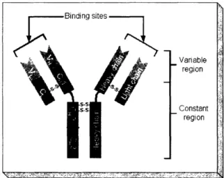
Antibodies belong to a class of proteins called immunoglobulins. They bind to anti-gens or other foreign substance in the body with high specificity, and are naturally produced by the body's immune system. Figure 1-1 shows the symbolic strcture of an

antibody. It is made up of two heavy and two light chains, which are linked together by disulfide bonds. The variable region indicated on Figure 1-1 is where the antibody interacts with its target antigen. The constant region, although has no affinity for antigens, is the part of antibody that interact with cells [22].

Figure 1-1: Structure of an antibody. Variable region

Constant region

:r-i.W : *.N. ,' . 5 p -S- ' '' ) ARI ge f-;- ,C-- '.I A' *--T--1:~~ - ' 9 'il=- ':-r : t

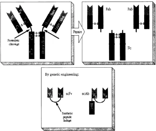
Different types of antibody fragments can be derived from full-length antibod-ies or produced by genetically modified cells. The nomenclature of antibody fragments is based on the part or parts of antibody that is included in the fragments. Examples of antibody fragments are shown in Figure 1-2.

Figure 1-2: Examples of Antibody fragments. Top: Fab and F. Bottom: scFv and

scAb.

Since antibodies are proteins themselves, they undergo proteolysis just like other proteins when the appropriate enzymes are present. For example, papain is an enzyme that is found to cleave antibodies at the hinge region, between CH1 and CH2 as shown in the top part of Figure 1-2, resulting in the separation of Fab (Fragment antigen binding) fragments from the F, (Fragment crystallizable) fragment.

Recent advances in genetic engineering has allowed the production of certain antibody fragments by genetically modified cells, such as bacteria, yeasts, hybridoma cells, insect cells, etc [15]. The DNA sequence for the specific antibody fragments can be inserted into the host cells by standard molecular biology techniques.

By genetic engineering: scFv scAb I Synthetic peptide 1ilr~ ,f,,f2- ' ; , S S 2

The use of antibody fragments have gained importance in the medical field recently, because of their wide potential as tumor targeting agents in areas such as radioimmunodetection and site-specific protein delivery. [13] This potential is mainly attributed to the reduced molecular weight (about 30 kDa) and size of antibody fragments.

Due to these properties, antibody fragments clear more rapidly from blood than whole antibodies. For the same reason, they are considered to have better tumor-penetrating properties. According to Damasceno et al., antibody fragments should also cause less or no immune response because of their shorter lifetime in the circulatory system. [10]

1.2 Heterologous recombinant proteins

Recombinant proteins are considered as "heterologous" if they are expressed in cells which they are not native to. For example, an enzyme found only in the mouse is

considered heterologous when it is produced in a bacterium.

Recombinant proteins have been widely studied, in both academic and com-mercial fields, because it has shown potential as a novel and versatile technique to produce proteins for medical purposes. Many research groups are studying production of recombinant proteins in various host systems, in order to develop cost-effective ways to produce any desired protein in large quantities, i.e. sufficient to obtain reasonable yield for characterization studies or clinical uses after downstream purification.

Current biotechnology allows genetic modifications to be made on organisms to express any protein as long as the protein is not cytotoxic. The DNA sequence of the desired protein can be inserted under a promoter or marker sequence. And in many cases, more than one copy of the foreign gene can be inserted into the organism's genome for higher productivity.

Bacteria have been widely used for expressing numerous heterologous proteins. However, being prokaryotes, they lack cellular functions that are only present in eukaryotes, e.g. secretion of proteins. As such, yeasts, being the simplest eukaryote,

has emerged as an alternative host for expression of eukaryotic proteins.

1.3 Pichia pastoris

This study focuses on the expression of an heterologous scAb (named AP39) by a yeast, Pichia pastoris. The Philips Petroleum Company was a pioneer in developing culturing protocols for P. pastoris, in 1970s. Studies to use P. pastoris as a host system for heterologous protein started only about a decade later. [4] Since then,

P. pastoris has become a successful host system for many different proteins over the

past two decades.

Cereghino et al. [15] published a list of heterologous proteins that have been expressed in P. pastoris. The list, which contains more than 200 proteins, includes proteins from bacteria, fungi, protists, plants, invertebrates, vertebrates (human and non-human), and virus.

Many other host systems have been employed to express antibody fragments. However, these host systems such as E. coli, Saccharomyces cerevisiae, etc. are be-coming less preferable for this application, compared to P. pastoris, due to a few advantages of P. pastoris over the aforementioned host systems. Some of the advan-tages will be discussed in the upcoming subsections.

For production of pharmaceutical molecules, it is ideal for the host system to be able to produce authentic or, at least, functional proteins, and with reasonably high productivity. With this consideration in mind, P. pastoris offers the fundamental safety prerequisite that it does not harbor undesirable substances such as pathogens or viral inclusions. [23]

Genetic manipulation

Genes in P. pastoris can be easily manipulated to include genes for heterologous proteins. Simple methods such as electroporation works well for this microorganism. Introduction of foreign genes into P. pastoris consists of three basic steps [15]: 1. Insertion of gene for target protein into vector; 2. Introduction of vector into host cells;

3. Examination and screening for transformed cells. Once the properly transformed cells have been correctly identified, they can be cultured in shake flask to maintain a stock of the host strain.

Genetic stability of P. pastoris has also made it a desirable host system for heterologous protein; loss of yield in P. pastoris was not significant even after several generations [23]. This is a crucial property for any host for recombinant protein. If the genome of a host system is unstable, then the yield of target protein will decrease with the number of times the cells have multiplied, or causes protein impurities to be produced, causing downstream purification process to be more difficult.

Nowadays, the P. pastoris expression system can be purchased as a commer-cially available kit. The host strain used for experiments in this thesis is obtained from Invitrogen Corporation (CA). Genes for heterologous proteins can be cloned into the genome of P. pastoris, under the inducible AOX1 promoter or the constitutive

GAP promoter.

Culture condition

P. pastoris is known to grow very well in inexpensive, defined medium. Culture

medium containing merely basal salts and carbon source within the pH range of 3-7

[3, 10] will keep P. pastoris viable.

P. pastoris is also known to grow well on different carbon sources, including

methanol, glycerol, glucose, sorbitol, etc. [9] This allows flexibility in medium opti-mization, since expression of different recombinant proteins may differ dramatically on different carbon sources.

High cell density

P. pastoris can grow up to much higher cell densities in both shake flasks and

biore-actors than its bacterial counterparts [1, 2, 3, 10, 17]. This is definitely a desirable feature, since higher cell densities in most cases imply higher recombinant protein

Post-translational modification

Unlike bacterial expression systems, P. pastoris is able to perform post-translational modifications that are often performed in higher eukaryotes, including glycosylation, folding, processing of signal sequences, and disulfide bond formation.

Such abilities allow recombinant proteins produced by P. pastoris to be se-creted directly into the supernatant, which is relatively protein-free in the first place. Since the recombinant protein is going to be the main protein present in the super-natant, the downstream purification process is greatly simplified. The target protein can be purified or concentrated easily by ultrafiltration.

Choice of promoters

When P. pastoris was first explored as a host for recombinant proteins, the foreign genes were usually inserted under the AOX1 promoter, which is a promoter that is tightly regulated by methanol [15]. The AOXI pathway is completely shut down when there is no methanol present in culture medium.

The main advantage of this promoter is that one can starve the yeasts of methanol in the first stage of fermentation to focus on building up cell density first. Once the cell density has reached the optimal level, methanol can be added to induce protein production. Another advantage of the inducible AOX1 promoter is its use for target proteins are harmful to the cells. Since the protein produced will depend on the level of methanol in culture medium, its production can be carefully manipulated so that it is kept below the toxic level. With these special properties, AOX1 became a popular promoter used for heterologous protein expression. [10]

Although the ability of P. pastoris to utilize methanol as its sole carbon source has rendered it useful for recombinant protein expression, excess methanol in culture medium can be toxic to the cells, so the concentration of methanol in culture has to be monitored closely in order to keep the viability of culture up [4]. This can be a difficult task, especially in shake flasks, where only offline monitoring is possible.

pro-moter. This is a constitutive promoter, and does not rely on the addition of methanol in culture medium to induce protein production. Many researchers have performed studies to compare it to the long-known AOX1 promoter. [20, 11]

The main advantage of this constitutive promoter is of course the elimination of the induction phase in fermentation and the starvation phase immediately before induction [4]. It also means that the lag phase that normally follows methanol in-duction would be eliminated, so the culture time required is now shorter. In other words, the use of a constitutive promoter leads to simultaneous biomass generation and protein production [12], which would make the process of protein expression more

efficient.

Furthermore, methanol is no longer required to be present in culture medium for recombinant protein expression, so the cells will no longer have the risk of undergo-ing methanol poisonundergo-ing. With these features, GAP is continually gainundergo-ing importance in recombinant protein production [27].

Chapter 2

Background

2.1 AP39 product formation

AP39 is a single-chain antibody fragments (scAb) produced by the P. pastoris in

subject. A scAb is a scFv with a human -light chain constant (HuC,) domain

attached to the C terminal. In the current study, the gene for AP39 is inserted into the P. pastoris genome under the constitutive GAP promoter.

AP39 molecules are secreted into the supernatant in two major forms: monomer (m 25 kDa) and dimer ( 50 kDa), with associative dimer being the desired product.

2.2 Growth conditions

Expression of recombinant proteins by P. pastoris depends on more than just a few factors, in both cultivation and cellular levels [21, 7]. However, only a few carefully chosen factors will be focused on in this study: agitation (oxygen level), initial glycerol concentration, salt concentration (osmotic stress). The chosen parameters are not the only factors on cell growth and recombinant protein production. Other factors that have been studied are, for example, cultivation temperature [18, 19] and carbon source

2.2.1 Agitation

The level of dissolved oxygen in culture depends highly on agitation, especially in shake flask cultures, where agitation is the only parameter that is closely related to dO2. Lee et al.found that, increasing DO from 10-30% to 30-50% increases final biomass by about 10%, and heterologous protein production by about three-fold [17]. Although this might not apply to all recombinant proteins, since each protein has its own characteristic behavior, dO2 does affect the redox potential in medium directly, which can in turn affecting protein production by P. pastoris.

2.2.2

Glycerol concentration

Glycerol is the sole carbon source for P. pastoris in SMMY medium, and is a limiting factor for biomass. It might also affect growth rate. Although there is little evidence that glycerol concentration plays a significant role in heterologous protein expression, its effect(s) on cell growth alone is significant and should be studied.

2.2.3

Salt concentration

This factor is also sometimes known as osmotic stress. In this study, the term salt concentration is specifically referred to as the total concentration of potassium phos-phate monobasic (KH2PO4) and potassium phosphate dibasic (K2HPO4). It is known to enhance protein production without compromising cell growth rate or biomass ac-cumulation in a few published studies [18, 10]. Shi et al.discovered that hypertonic media containing 0.35M of salt led to increase in scFv production by several-fold [7].

2.3 Factorial study

The concept of factorial experimental design has been gaining importance in many scientific fields recently, due to its ability to study trends for multiple factors and their combined effects in significantly fewer number of experiments than traditional methods. This has also simplified studies where first-order analysis is insufficient.

2.3.1 Central composite design (face-centered)

Central composite design, an extension of factorial study, was employed in a few published studies to investigate, for example, recombinant protein expression [24] and protein stability [25]. The difference between CCD and ordinary 23 factorial study is that CCD includes a number of axial and center runs in addition to the factorial runs. A few types of CCD are commonly used, such as spherical, Box-Behnken, and face-centered [26]. Face-centered (fc) CCD is the type of CCD carried out in this study.

By including axial and center runs in the CCD, quadratic terms can now be incoporated in the model. [26] The parameters that need to be specified concerning the CCD are:

1. a, the distance of axial runs from design center.

2. nc, the number of center points.

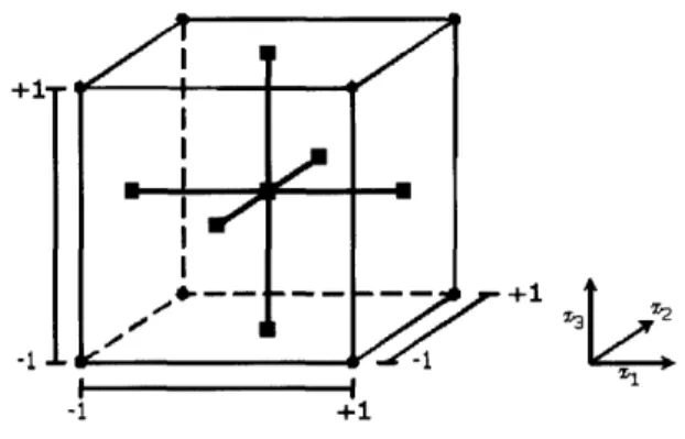
The parameter a is dictated solely by the area of interest. For example, in this study where fcCCD is used, oa = 1, and in a spherical CCD, a = vA, where k is the number of factors studied. Center runs are included in CCD to provide variance for prediction. In general, the recommended nc is smaller for fcCCD than in spherical CCD. In this study, no - 1. Figure 2-1 below gives an overview of the experimental design that will be the object of discussion for the rest of the paper.

2.3.2 Response surface regression

Response surface regression is very often combined with CCD experiments, and when-ever there is a response, or observed result, that depends on k independent variables (e.g. agitation, glycerol concentration, and salt concentration in this case).

The relationship between the response and the independent variables is char-acterized by a regression model. Linear models are the most commonly used model for regression. The regression model can be fitted to a set of observed responses,

_e i +1--1. --m 13+1 -i I I -1 +1

Figure 2-1: The 23 factorial design with fcCCD.

and can then be used to predict responses for any given conditions within the region studied.

2.4 Objectives

In the present study, three responses: the growth of P. pastoris (biomass and growth rate) and production of AP39 by the yeast (protein concentration by BCA assay) were to be investigated in a CCD factorial study. The three factors chosen to be investigated were: agitation, initial glycerol concentration, and initial salt concentra-tion.

The purpose of this study is to elucidate the dependence on the selected re-sponses on the three growth parameters listed above and their interactions. So that, as a result, Production of heterologous scAB, AP39, can be optimized on the culture level based on the improved understanding of the behavior of P. pastoris culture.

I | W 'I I I I W-000, / 4 I o ,P 0 m I _.,., l - -: ';2 I.4- j ~~~crC~~~~~~

IC ,~~~~~~1

Chapter 3

Experimental Procedure

3.1 Materials

3.1.1

Organisms

The P. pastoris host strain X33 was received from Berlex Laboratories, Inc. (Rich-mond, CA). The cryogenic vials containing the cells were stored at -80°C immediately upon arrival. This host strain of P. pastoris was genetically modified to contain a single copy of AP39 gene under the constitutive GAP promoter.

3.1.2 Chemicals

The chemicals used in all the experiments performed are purchased from Sigma-Aldrich, Mallinckrodt Baker, and BD Biosciences. All chemicals used were of reagent grade unless otherwise stated.

3.1.3 Culture medium

This section outlines the composition of solutions used in shake flask cultures. The biotin stock solution was made in bulk ahead of time, and can be kept at specified conditions for extended period of time.

0.2% w/v Biotin stock solution contains 0.2% biotin dissolved in 0.1N

NaOH solution. It is filter sterilized through 0.22 ,um filter, and stored in 0.5 mL aliquots at -20°C.

SMMY culture medium contains 2% w/v Soytone, 1% w/v Yeast Extract,

1.36% w/v Yeast Nitrogen Base without Amino Acids, 1.4% w/v potassium phos-phates (KPO4), and 2% v/v glycerol dissolved in DI water. The pH was adjusted to pH 5.5 using 80% phosphoric acid prior to filter sterilization through 0.22 Atm filter. After filtration, 0.2% biotin stock solution was added to SMMY medium sterilely to reach a final concentration of 0.005% v/v.

3.2 Expansion of glycerol cell bank

A glycerol cell bank was expanded from the frozen cryogenic vials of P. pastoris (at -80°C) received from Berlex. The cell bank was expanded using 500 mL baffled flasks as shown in Figure 3-1 . The same kind of shake flasks were used in all other experiments that are described in later sections.

Figure 3-1: Baffled flask used for P. pastoris culture. Corning #4446-500.

SMMY culture medium was prepared according to instructions described above shortly before inoculation of shake flasks. Prior to inoculation, the shake flasks were covered with filter paper and aluminum foil, and autoclaved at 121°C for 45 minutes.

1

http://catalog2.corning.com/Lifesciences/productdetails.aspx?p=Containers401 15&id=4446

100 mL of SMMY culture medium was first sterilely transferred to each baffled flask. Then, 100 ttL of thawed cells from the cryogenic vials was added into each of the flasks with a 200 ,iL pipettor, using sterile technique. The shake flasks were incubated in a shaker for 96 hours (4 days) at 30°C and 125 rpm.

At the end of the 4-day period, a sample of about 1 mL was taken from each shake flask to ensure that the cell density reached the desired level by measuring its OD₆₀₀. Then, 22.2 mL of 50% v/v glycerol solution in DI water (filter sterilized) was added to each shake flask. The flasks were swirled to mix the contents. The cells are then transfered to cryogenic vials in 1 mL aliquots, and stored at -800C for use in later experiments.

3.3

Shake flask cultures: Central Composite

De-sign

A 3-factor (k=3), 3-level face-centered central composite design (fcCCD) was em-ployed in this study, involving 15 experiments in a full factorial design. The study was made up of eight (8 = 2k=3) factorial points, six axial points (na=2 points on the

axis per factor at a distance of (a = 1), and one (n,=l1) center point. The experimental design can be visualized geometrically as in Figure 2-1.

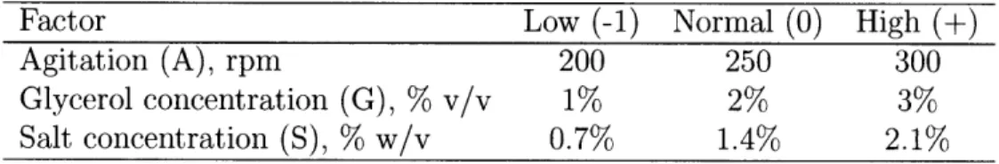
As mentioned in Section 2.4, the independent factors studied were agitation, glycerol concentration in SMMY culture medium, and salt concentration in SMMY2_. The range in which they are studied were shown in Table 3.1.

Table 3.1: Factors studied and their ranges under investigation.

Factor Low (-1) Normal (0) High (+)

Agitation (A), rpm 200 250 300

Glycerol concentration (G), % v/v 1% 2% 3% Salt concentration (S), % w/v 0.7% 1.4% 2.1%

The conditions for low and high glycerol and/or salt concentration(s) were

2_{Total concentration of KPO}

experimented by making SMMY medium according to the protocol, but adjusting the amount of glycerol and/or KPO4 to achieve the desired concentrations. For potassium phosphates, the ratio of monobasic to dibasic salts was kept constant while adjusting the salt concentration, only the total amount of salt added was adjusted.

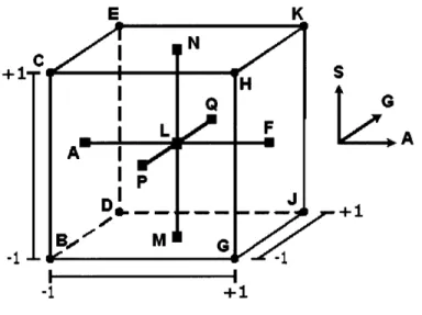
Figure 3-2 is modified from Figure 2-1, to illustrate the geometric layout of experimental conditions listed in Table 3.2. The round black dots at the vertices of the cube in Figure 2-1 represent factorial experimental conditions, and the small black squares represent the axial and center points.

Each of these conditions was run in duplicates to reduce experimental and random errors, and to improve precision of data. Table 3.2 shows the independent factors (xi), in their coded and uncoded forms, in an experimental design matrix.

+1 -1 -C S

L

G

t

A

,,+I

Figure 3-2: The 23 _{factorial design with fcCCD (with labels).}

The shake flask cultures were run in three batches. Those runs with the same agitation rate were incubated at the same time. The first batch includes setups A,

B, C, D, E; second batch F, G, H, J, K; and third batch L, M, N, P, Q.

Each shake flask culture contained 100 mL of SMMY culture medium, and was inoculated with 100 /iL of thawed cells from the glycerol cell bank. Starting from the moment the shake flask was inoculated, 2-3 mL of sample was collected

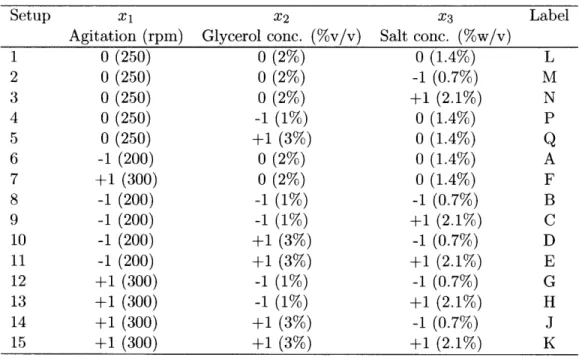
Table 3.2: Design matrix of 3-Factor-3-level fcCCD

Setup X1 X2 X3 Label

Agitation (rpm) Glycerol conc. (%v/v) Salt conc. (%w/v)

1 0 (250) 0 (2%) 0 (1.4%) L 2 0 (250) 0 (2%) -1 (0.7%) M 3 0 (250) 0 (2%) +1 (2.1%) N 4 0 (250) -1 (1%) 0 (1.4%) P 5 0 (250) +1 (3%) 0 (1.4%) Q 6 -1 (200) 0 (2%) 0 (1.4%) A 7 +1 (300) 0 (2%) 0 (1.4%) F 8 -1 (200) -1 (1%) -1 (0.7%) B 9 -1 (200) -1 (1%) +1 (2.1%) C 10 -1 (200) +1 (3%) -1 (0.7%) D 11 -1 (200) +1 (3%) +1 (2.1%) E 12 +1 (300) -1 (1%) -1 (0.7%) G 13 +1 (300) -1 (1%) +1 (2.1%) H 14 +1 (300) +1 (3%) -1 (0.7%) J 15 +1 (300) +1 (3%) +1 (2.1%) K

approximately every 12 hours (up to 96 hours), for OD600 and DCW measurements.

At the end of the 96-hour incubation period, in addition to the sample taken for OD60 0 and DCW assays, the content of each shake flask was transfered to 50 mL centrifuge tubes, where it was centrifuged at 3000 rpm for 15 minutes. After that, the supernatant was kept at 4C in a refrigerator until protein assays were performed, and the cell pellet was discarded.

3.4

Biomass assays

3.4.1 Optical density at 600 nm

Optical density is one of the methods to measure cell concentration in culture. Ab-sorbance of the cell culture is measured using an UV/Visible spectrophotometer, at A = 600 nrn (OD₆₀₀). Cells in suspension absorbs light at 600 nm, and the OD600 reading is directly proportional to the cell density in culture.

Most UV/Visible spectrophotometers have a narrow range of reading (typically 0.1-1.0) beyond which readings are curvilinear. Therefore, when the OD600 readings

of culture is larger than 1, 1:10 dilution will have to be made using deionized water (DI water). Multiple 1:10 dilutions are sometimes required for very high cell density, in order to obtain an OD6 00 reading within range.

3.4.2

Dry cell weight

Dry cell weight (DCW) is an universal measure for cell density in culture, because it does not rely on readings provided by specific equipment, and can be done on all types of cultures. A culture sample is transfered to a preweighed 1.5 mL EppendorfrM tube, in which it will be centrifuged to remove the supernatant, and then washed twice to remove soluble components, such as salts and culture medium components. Cells can be washed by resuspending the cell pellet in DI water and then centrifuging again.

The washed cell pellet is then dried in an oven set to 60-70°C until the cells are completely dry, which is indicated by constant mass. The DCW can be calculated by

DCW = (Mass of eppendorf tube + dried cells) - (Mass of empty tube) (3.1)

3.5 BCA Protein assay

Bicinchoninic acid (BCATM) Protein Assay kit from Pierce was used to quantify total protein concentration in supernatant from each experiment at the end of the 96-hour incubation. As mentioned in Section 1.3, P. pastoris does not secrete protein into supernatant under normal conditions, nor is cell lysis required to retrieve target pro-tein. Thus, the proteins present in supernatant can almost be completely attributed to AP39, which is the protein designated to be secreted.

In this study, the 96-well microplate procedure was used to quantify proteins in supernatant collected from each shake flask, after 96 hours of incubation. Work-ing reagent (WR) is prepared by mixWork-ing the preformulated Reagents A (contains sodium carbonate, sodium bicarbonate, BCA detection reagent, sodium tartrate in 0.1N sodium hydroxide) and B (contains 4% copper (II) sulfate) in the ratio of 50:1.

Protein standards used for standard curve calibration was BSA3 standards that was provided in the BCA assay kit. BSA was used to calibrate the assay. Due to limita-tion of the microplate reader, the range of BSA concentralimita-tion used for calibralimita-tion was narrowed down to 125-1000 jtg/mL. Triplicates of each standard were measured, but only duplicates were measured for each sample, due to the large number of samples. For both BSA standard and sample measurements, 25 1uL of standard, sample, or blank replicate was pipetted into a microplate well. Supernatant samples were diluted 10 times with DI water to ensure that protein concentration lies within the working range. Since DI waterwas the solvent used to dilute samples, it was also used as blank in colorimetry measurement. Then 200 L of WR was pipetted into each well containing a blank, standard or sample replicate. The contents in each well was slightly mixed horizontally by gentle sideways motion. Then, the microplate was covered and incubated at 37°C for 30 minutes.

After incubation, the microplate was removed from the incubator, and left to cool to room temperature, to quench the BCA reaction. Absorbance was measured at 562 nm on a plate reader after cooling.

3

Chapter 4

Calculations

4.1

ANOVA

The method of ANOVA (Analysis Of Variance) was employed to preliminarily deter-mine whether the model proposed for each of the responses (biomass, growth rate, and BCA protein concentration) is appropriate. For this part of analysis, only the data obtained from the eight factorial points, which are represented by the vertices of the cube in Figure 2-1, were considered. The axial and center points will be included later in response surface regression.

In the analysis to follow, including those in later sections, 'A' stands for agita-tion (in rpm of shaker), 'G' stands for initial glycerol concentraagita-tion of SMMY medium (in % v/v), and 'S' stands for initial salt (KPO₄) concentration of SMMY medium (in % w/v). These are the factors under investigation in this study. Any combination of the above symbols represents the interaction between those factors.

4.1.1

Main effects

The formula for main effect of A can be derived by first considering the difference between the average of the four experimental conditions where A is at high level (i.e.

YA-), and four experimental conditions where A is at low level (i.e. A-).

the notations in Table 4.1, the four conditions where A is at high level are a, ag, as, and ags. Similarly, the four conditions where A is at low level are (1), g, s, and gs. These symbols represent the total of all n observations at that particular experimental condition, and n = 2 in this study.

17.Q !-,a + -.;. --, S I (1) I

as

a

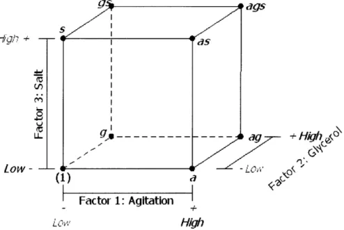
Figure 4-1: Geometric representation of the 23 factorial design.

Table 4.1: Notations for total observations in 23factorial design.

Labels Agitation (A) Glycerol (G) Salt (S)

(1) - - -s - - + g - + -gs - + + a + - -as + - + ag + + -ags + + +

Therefore, the effect of A can be written as follows:

[a + ag + as + ags - (1) - g - s - gs]

4n (4.1)

The quantity in square brackets in the above equation is known as the contrast of A.

Is I . l I

0

"I

IZ

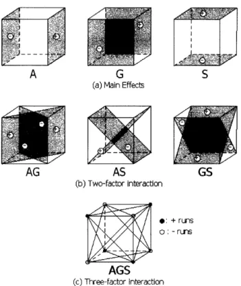
Figure 4-2(a) illustrates the main effect in a 23 _{factorial design.}

The main effects of G and S are derived using similar methods.

G [g + ag + gs + ags - (1) - a -s - as] (4.2)

4n

[s + as + gs + ags - (1) - a - g- ag]

4n

The two-factor intereaction effects (e.g. AG) can be computed in a similar way, by first considering the difference between the average A effects at high and low levels of G. When G is high, the average A effect is [(ags - gs) + (ag - g)]/2n; when G is low, the average A effect is [(as - s) + (a - (1))]/2n. The difference between these two average A effects is [ags - gs + ag - g - as + s - a + (1)]/2n. Since the AG interaction is half of this difference,

AG = [ags + ag + s + (1) - gs - g - as - a]

(4.4)

4n Following similar logic, and from Figure 4-2(b)

AS = [ags + as + g + (1) - gs - s - ag - a]

(4.5)

4n

GS = [ags + gs + a + (1) - as - s - ag -g]

(4.6)

The three-factor interaction (AGS interaction) is defined as the average differ-ence between the AG interaction at high and low levels of S. At high level of S, the AG interaction is [(ags - gs) - (as - s)]/4n; at low level of S, the AG interaction is

[(ag - g) - (a - (1))]/4n. Therefore,

AGS = [ags + s + g + a - ag - as - gs - (1)]

(47)

4n

Equations 4.1 to 4.7 summarizes the main effect and interactions between the three factors.

A G S

(a) Main Effects

AG AS (b) Two-factor interaction GS *: + runs : -rus AGS (c) Three-factor interaction

Figure 4-2: Contrasts corresponding to main effects and interactions between factors.

4.1.2

Sum of squares

In Equations 4.1 to 4.7, the quantities in square brackets are called contrasts. These contrasts will be used to calculate sum of squares (SS) for each of these effects. In this 23 design with n 2 replicates, the sum of square of any effect is

(Contrasti)2

8n (4.8)

where i = A, G, S, AG, AS, GS, AGS.

The total sum of squares (SST) is the sum of the squared differences between each observation or response (Y) and the overall average:

(4.9)

SST -=

(Y - overall)2

all

effects from SST:

SSE

= SST - (SSA + SSG + SSs + SSAG + SSGS + SSGS + SSAGS)

(4.10)

The error sum of squares is composed of the pure error arising from the replication of the factorial points.

Once all the sum of squares are calculated, ANOVA can be performed on the observed data for each response, as shown in Table 4.2. Mean squares of all the effects and error are calculated by dividing the sum of square with the corresponding degree of freedom (df).

If the following assumptions are made: (1) the model is adequate, and (2) the errors are normally and independently distributed with constant variance, then the F0 statistic for each effect, which is defined as F = MSeffect/MSE, are distributed as F, with the critical region at the upper tail of the distribution, i.e. higher values of F0 statistics implies high probability of that effect being significant in the model.

4.1.3 Hypothesis testing

The model sum of squares can be calculated by summing the SS of all effects (see

Table 4.2:

SSode = SSA + SSG + SSS + SSAG + SSGS + SSGS + SSAGS

(4.11)

The degree of freedom of SSModel is 7, since there are seven main effects and interac-tions altogether. Therefore, MSMoI,dl SSAIO,de/7, and thus the statistic

MSModel

F

is

(4.12)

MSE

will be testing the hypotheses

Ho :3A = aG = s = -AG = AS = OGS -= AGS = 0

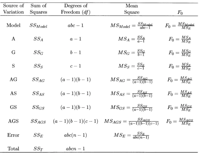
Table 4.2: The Analysis of Variance table for 3-factor fixed effects model. (Note: a,

b, and c are the number of levels in factors A, G, and S, respectively; n is the number

of replicates run for each experimental condition. In this case, a = b = c = n = 2.)

Source of Sum of Degrees of Mean

Variation Squares Freedom (df) Square F0

Model SSModel abc - 1 MSModel SSMdel _abc- Fg = MSMdel_MSE

A SSA a-i MSA = SSa _a-1 Fo = MSA_MSE

G SSG b-1 MSG = SS _{SGb- 1} F = MSG_MSE

S SSs c-i MSs

=S-

AG _AS SSAG _{SSAG (a- 1)(b- 1)} (a-l)(b-) MSSSAG _MSAG MSAG

= (a-1)(b-1) Fo = MSE

AS

-~1)(b

- 1)

GS SSGS (a- )(b- 1) MSGS (a- _(a-1)(b-1) SS F = ₀ MSGS

- MSE

SSE

Error SSE abc(n- 1) MSE = ab(n-1)

Total SST abcn - 1

For a test at 95%, if Fo > F0.05,,, 2 (where l =- dfModel = 7 and v2 = dfE = 8),

then it is reasonable to conclude that at least one variable has nonzero effect. Next, each of the individual effect and interaction will be tested in the same way for its significance in the model using the individual Fo statistic from ANOVA as listed in Table 4.2. Note that for a stricter test, e.g. at 99%, Fcrit will be larger. In other words, it is harder for the Ho hypothesis to be rejected. This is attributed to the fact

that Type I error 1 is less likely to occur in a 99% test (e.g.) than 95%.

1_{Type I error is the error when the null hypthesis, Ho}

0, is rejected, but in reality it is actually

4.1.4 R

_Statistics

An R2 statistic can be evaluated as follows SSModel

R2 SSModel (4.13)

SST

This statistic measures the proportion of total variability accounted for by the model. From its formula, it can be seen that the closer this R2 _{is to unity, the 'better' the}

model fit the data.

However, the value of R2 always increases whenever additional factors are added to the model, even if those additional terms are non-significant. Therefore, the adjusted R2, which is defined as

SSE/dfE

R d- 1- SS /dfT' (4.14)

sometimes serves as a better measure for accuracy of model, since it takes into account the " 'size"' of the model. The value of RAdj statistic will actually decrease if non-significant terms are added to the model. Similarly, it can be inferred that, the value of adjusted R2 will increase if non-significant terms are eliminated from or significant terms are added to the model.

With this property, R2Adj can be a helpful indicator when attempting to refine the proposed models. Also, when R2 _{and Rdj differ dramatically, it is an indication}

that non-significant terms are present in the model.

4.2 Response surface regression (RSREG)

The regression model for predicting all the responses (biomass, growth rate, and BCA protein concentration) is

Y

-=

3o

+ AA + GG + SS + 3AGAG

+ PASAS

+ /GsGS +

AAGSAGS4.15)

where in Equation 4.16, the model is being expressed in terms of coded variables:

-

2

(Xma - Xmin)

(4.17)

and x1 2 = XlX2, x13= x1X3, etc.

To fit the proposed model to experimental data, the parameters in the model (the d's) have to first be estimated. They can be estimated by

-=

= E allY

The estimated d are used as initial guesses for model fitting. The term residue is defined as the vertical distance between the observed and predicted Y values:

Residue = Yobs - z

where Y is the predicted value of Y at the same condition as Yobs; and Y = 0o+i i3x. Regression of mathematical models is achieved by minimizing the sum of squared residues.

Sum of squared residues:

all conditions

all conditions

Surface and contour plots of the predicted responses can be generated after the models have been fitted to the data.

- 2

i

Chapter 5

Results

5.1 Correlation between OD

600

and DCW

Optical density at 600 nm (OD600) and dry cell weight (DCW) are both measures of biomass, and they should be linearly correlated, because both these quantities are directly proportional to cell density in culture. During all shake flask experiments, culture samples from each shake flasks were taken approximately every 12 hours, and

both OD60 0 and DCW were measured. This was done to ensure data from both low

and high cell densities were covered when determining the correlation.

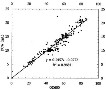
Linear regression was performed by Microsoft Excel on all the OD600 and DCW

data collected as shown in Figure 5-1, and the correlation is given by

DCW (g/L) = 0.2457 x OD60 0 - 0.0272 (5.1)

with a correlation coefficient, R2 = 0.9664.

Since OD600 measurements can be very different depending on the equipment used, DCW is a preferable measure of biomass compared to OD₆₀₀. Therefore, in all the analyses to follow, the biomass data were DCW in g/L converted from OD600.

0 20 40 60 80 100 7c o 20 o 15 U 10 5 0 20 15 10 No 0 20 40 60 80 100 OD600

Figure 5-1: Correlation between DCW (in g/L) and OD600

5.2

Shake flask cultures

80 70 60 'D 40

a

Figure 5-2: Typical temporal profile of OD600 and DCW.

Figure 5-2 shows a typical profile of optical density and dry cell weight over time during the duration when the shake flask was incubated. This specific plot shows a lag phase of about 8 hours at the beginning of incubation (labeled 1 in the profile), followed by an exponential growth phase from 8-48 hours (labeled 2). The biomass stopped increasing after 48 hours, and the same cell density was maintained until the

end of incubation (labeled 3). Such profiles for OD600 and DCW for all experiments are shown in Appendix B

It is important to note that the exact durations for lag phase and exponential growth phase were not the same in all experiments, since it depends largely on the experimental condition.

5.3 Face-centered central composite design

Table 5.1 summarizes the data obtained from fcCCD. Since each experimental con-dition was duplicated (with the exception of setup #2, because one of the flasks was broken halfway through the experiment), the mean and standard deviation were calculated for each of the conditions.

Table 5.1: Results from 3-Factor-3-level fcCCD response surface analysis. (Biomass is given in g/L; Growth rate in hr-1; and BCA Protein concentration in mg/mL.)

Setup (A, G, S) (Y1) Biomass Std Dev (Y2) Rate Std Dev (Y3) BCA+Std Dev

1 (0,0,0) 15.85 i 0.59 0.4329 i 0.0265 7.909 i 0.068 2 (0,0,-i) 13.77 i 0.66 0.3419 i 0.0449 7.743 i 0.000 3 (0,0,+1) 14.58 ± 0.18 0.3929 ± 0.0081 7.278 ± 0.133 4 (0,-1,0) 10.41 i 0.28 0.3946 i 0.0029 6.676 i 0.133 5 (0,+1,0) 17.28 ± 0.01 0.2858 ± 0.0030 7.643 ± 0.043 6 (-1,0,0) 14.85 i 0.29 0.2313 ± 0.0148 6.953 ± 0.019 7 (+1,0,0) 15.87 i 0.08 0.3721 i 0.0570 6.359 0.043 8 (-1,-1,-1) 13.33 i 0.55 0.2816 ± 0.0227 7.346 ± 0.117 9 (-1,-1,+1) 12.71 ± 0.19 0.2357 ± 0.0550 6.660 ± 0.093 10 (-1,+1,-1) 18.64 i 0.37 0.2885 ± 0.0152 6.767 ± 0.127 11 (-1,+1,+1) 18.48 2.62 0.2294 i 0.0122 7.200 i 0.182 12 (+1,-1,-1) 11.18 ± 0.32 0.3985 ± 0.0160 6.628 ± 0.040 13 (+1,-1,+1) 10.96 ± 0.12 0.4064 ± 0.0034 6.499 ± 0.173 14(-+1,+1,-1) 19.28 ± 0.11 0.4245 ± 0.0416 6.800 0.142 15 (+1,+,1+1) 19.97 0.20 0.4850 0.0160 6.844 0.074

5.4

Statistical Analysis: ANOVA

ANOVA (analysis of variance) was employed to study the accuracy of the proposed model, as outlined in Section 4.1. First of all, all effect estimates and sum of squares for each response (Yi) were calculated. The calculations are summarized in Table 5.2.

Table 5.2: Effect estimate summary. Y1 = Biomass

Factor Effect Estimate

A -0.4392 G 7.0493 S -0.0782 AG 1.5100 AS 0.3165 GS 0.3403 AGS 0.1093 Pure Error Total Y2 = Growth Rate

Factor Effect Estimate

A 0.1698 G 0.0263 S -0.0092 AG 0.0260 AS 0.0433 GS 0.0099 AGS 0.0164 Pure Error Total

Y3 = BCA Protein Conce

Factor Effect Estimate

A -0.3007 G 0.1195 S -0.0846 AG 0.1392 AS 0.0420 GS 0.3226 AGS -0.2363 Pure Error Total

Sum of Squares % Contribution

0.7715 0.36% 198.7727 91.55% 0.0245 0.01% 9.1208 4.20% 0.4008 0.18% 0.4632 0.21% 0.0478 0.02% 7.5117 3.46% 217.1130 100%

Sum of Squares % Contribution

1.15x10- ' 2.77x 10-3 3.35 x 10-4 2.71x10- 3 7.51 x 10-3 3.90 x 10-4 1.08x 10- 3 6.18 x10- 3 0.1363 .ntration Sum of Squares 0.3618 0.0572 0.0286 0.0775 0.0071 0.4162 0.2234 0.1287 1.3005 84.61% 2.03% 0.25% 1.99% 5.51% 0.29% 0.79% 4.54% 100% % Contribution 27.82% 4.39% 2.20% 5.96% 0.54% 32.00% 17.18% 9.90% 100%

-With the individual sum of squares calculated, ANOVA can be performed on the overall model for all the responses, testing the hypotheses stated on P.39.

Ho A = /3G = 3S = ACG -3AS -= /GS = AGS = 0 (5.2)

H1 : at least one /3# 0 (5.3)

The critical region for this test of hypothesis at 95% is Fo > F.05,7,8 = 3.50, i.e.

Ho would be rejected (i.e. at least one Q 5 0) if the Fo calculated is greater than

3.50 (degrees of freedom of each model and the corresponding error are 7 and 8, respectively). Table 5.3 shows that Ho for all three responses were rejected, indicating that at least one variable has a nonzero effect on the responses.

Table 5.3: ANOVA for preliminary mathematical models.

Response SSModel MSModel F0 Reject Ho? R2 RAd

Biomass 209.6013 29.9430 31.8893 Yes 0.965 0.935 Growth rate 0.1301 0.0186 24.0522 Yes 0.955 0.915 BCA Protein Conc. 1.1718 0.1674 10.4031 Yes 0.901 0.814

Although the presence of nonzero effects has been established by ANOVA, it is shown in Table 5.3 that R2dj < R2 in all models. This is an indication that insignificant terms are present in all the models. Therefore, hypothesis testing for individual effects were to be carried out in order to exclude non-significant terms in the models. F₀ statistics were calculated as described in Table 4.2. The critical region for individual effects' hypothesis testing at 95% is F0 > F0.0 5,1,8= 5.32 (degree

of freedom for each effect is 1).

Table 5.4 summarizes the results from ANOVA for all the individual effects and interactions for all responses. A few factors had Fo that were smaller than F0.0 5,1,8, but

were still in the same order of magnitude. These effects are indicated by a question mark under the "Reject Ho?" column. They are also included in the model to be fitted, since these factors might reject Ho in a test less strict, and they might have some effect on the responses.

Table 5.4: Results from ANOVA.

(1) Biomass

Sum of Degree of Mean

Factor Squares Freedom Square F0 Reject Ho?

A 0.7715 1 0.7715 0.8217 No G 198.7727 1 198.7727 211.6927 Yes S 0.0245 1 0.0245 0.0261 No AG 9.1208 1 9.1208 9.7136 Yes AS 0.4008 1 0.4008 0.4269 No GS 0.4632 1 0.4632 0.4933 No AGS 0.0478 1 0.0478 0.0509 No Pure Error 7.5117 8 0.9390 Total 217.1130 15 (2) Growth Rate

Sum of Degree of Mean

Factor Squares Freedom Square F0 Reject Ho?

A 1.15x10 -1 1 1.15x10-1 149.2219 Yes G 2.77x10- 3 _{1 2.77x 10}-3 _{3.5790 Yes?} S 3.35 x 10-4 1 3.35 x 10- 4 0.4334 No AG 2.71x 10- 3 1 2.71x10- 3 3.5066 Yes? AS 7.51x 10- 3 1 7.51x10- 3 9.7202 Yes GS 3.90x 10- 4 1 3.90x 10- 4 0.5042 No AGS 1.08 x 10- 3 1 1.08 x 10- 3 1.4000 No Pure Error 6.18x 10- 3 8 7.73x 10- 4 Total 0.1363 15

(3) BCA Protein Concentration

Sum of Degree of Mean

Factor Squares Freedom Square F0 Reject Ho?

A 0.3618 1 0.3618 22.4839 Yes G 0.0572 1 0.0572 3.5519 Yes? S 0.0286 1 0.0286 1.7792 No AG 0.0775 1 0.0775 4.8156 Yes? AS 0.0071 1 0.0071 0.4391 No GS 0.4162 1 0.4162 25.8669 Yes AGS 0.2234 1 0.2234 13.8849 Yes Pure Error 0.1287 8 0.0161 Total 1.3005 15

Once the significant factors for each response were selected, another round of ANOVA was run on the now reduced models, to see if the models would now fit the data better. This can be done by comparing the values of Rdj for the full and reduced models. As discussed in Section 4.1.4, the value of R2dj would increase if non-significant terms were removed from the model, even though the ordinary R2 would always decrease when any effects are removed.

For the second round of model ANOVA, a few changes were added to the calculations. The error term now includes the effects that were screened out of the model, i.e. those effects that were found insignificant in Table 5.4. Therefore, the error sum of squares (SSE) and its degree of freedom now equal

SSE (new) = SSE (old) + E SS (non-significant) (5.4)

dfE (new) = dfE (old) + E dfi (non-significant) (5.5)

In the reduced models, the term SSE is made up of two parts. The first part being the pure error arising from the replications of each experiment, and the second part being the lack of fit component, consisting the sums of squares for the effect or interactions that were dropped from the original models.

So the revised MSE will now equal to new SSE divided by its new degree of freedom. The new values of SSModdl and SSE will be used to calculate the two R2 statistics from the same formulae in Section 4.1.4.

The results from ANOVA for the reduced models are summarized in Table 5.5. It shows that the reduced models of biomass and growth rate has almost the same

RAdj values as their respective full models, with the difference being only 1-2%. On

the other hand, the reduced model of protein concentration had a R2dj that is 8% lower than that of the full model: 0.746 compared to 0.814.

Table 5.5: Model Analysis of variance: Comparison between full and reduced models.

Response Model Type SSAodel MSModel FO Reject Ho? R2 Rd

Biomass Full 209.601 29.943 31.89 Yes 0.965 0.935

Reduced 207.893 103.947 146.57 Yes 0.958 0.951

Growth rate Full 0.130 0.019 24.05 Yes 0.955 0.915

Reduced 0.126 0.042 46.69 Yes 0.921 0.901

Protein Conc. Full 1.172 0.167 10.40 Yes 0.901 0.814

Reduced 1.059 0.265 12.03 Yes 0.814 0.746

5.5 Mathematical modeling: RSREG

The reduced model for each response was fitted to the observed data by minimizing the sum of squared residue from observed points to fitted points (Equation 4.20)

The models resulting from regression are: Biomass (g/L):

Y = 15.144 + 3.506x2 + 0.755x1x2 (5.6)

Growth rate (hr-1):

Y2 = 0.347 + 0.082x1 - 0.000358x2+ 0.013x1x2 + 0.022x1x3 (5.7)

BCA Protein concentration (mg/mL):

Y3 = 7.020 - 0.180x1 + 0.145x2 + 0.070xx 2 + 0.161x2x3- 0.118xlx2x3 (5.8)

where x1, x2, and X3 are the coded variables representing agitation, glycerol

concen-tration, and salt concentration respectively. The coefficients are summarized in Table 5.6 for easier comparison.

Selected surface and contour plots with interesting properties are displayed in this section. Appendix D contains more surface and contour plots from the fitted models with different parameters fixed.

Table 5.6: Coefficients for fitted models by RSREG.

Coefficient Y1 (Biomass) Y2 (Growth rate) Y3 (Protein conc.)

/30 15.144 0.347 7.020 131 0 0.082 -0.180 /32 3.506 -0.000358 0.145 /33 0 0 0 /12 0.755 0.013 0.070 P13 0 0.022 0 /323 0 0 0.161 /123 0 0 -0.118

5.5.1

Biomass

According to Figure 5-3 biomass is a linear function when agitation is fixed, with biomass increasing with glycerol concentration. This can be deduced from the fitted model for biomass (Y1) that when agitation (xi) is fixed, the model is reduced to a linear function:

Y1 = 15.144 + (3.506 + 0.755x1)x2

Figure 5-3 also shows that the slope of increasing biomass with glycerol con-centration was the steepest when agitation was highest at 300 rpm, where biomass increased from t 1 g/L to more than 19 g/L, which is almost a two-fold increase. On the other hand, the slope was the least steep when agitation was lowest at 200 rpm, where increase of biomass was from 12.5 g/L to about 18 g/L, which was a 44% increase.

5.5.2 Growth rate

The patterns of growth rate at different levels of agitation, unlike biomass, are differ-ent at all three levels shown, as illustrated in Figure 5-4, that the contour lines are in different directions for all three levels of agitation. At 300 rpm (high agitation), growth rate was the highest at high salt and glycerol concentrations (0.47 hr-1). However, the pattern was reversed at 200 rpm (low agitation), where growth rate was the highest at low salt and glycerol concentrations (0.445 hr-1).

ITS~ ,,,.,, m s if ... ... :''. 1 ''''''''': ... ': ' .. 17 0 _{--- ! -... ...} 15 . 1 ... ... 14 -. 5 .-- '... - - -1 -13 O _ , -1 -1 c -) -1 -0.5 0 0.5 1

aE,,,,,...-n18

.

.

li

0.5

_'~

-1..

Concentration Concentration Glycerol Concentration (coded)

(coded) (coded)

Figure 5-3: Surface (left column) and contour (right column) plots of biomass (g/L) at low, netural, and high levels of agitation (A).

At agitation of 250 rpm, the predicted range of growth rate was 0.335 to 0.36 hr- 1, which was significantly lower than the range predicted for both high and low agitation rates: 0.41-0.45 hr-1 at 200 rpm and 0.39-0.47 hr- 1 at 300 rpm.

5.5.3 Protein production

The model for protein concentration is the only model in this study that has a third order term Xlx2x3. It is also the only model that has a stationary point in the region of study. Figure 5-5 shows that protein concentration has a saddle point at both 200 and 250 rpm.

At A = 200 rpm, protein concentration was predicted to increase at both higher and lower glycerol and salt concentrations, as shown in the first contour plot in Figure 5-5, that predicted protein concentration was 7.2 mg/mL at high glycerol

L- 20 to 0 15 1 10 o Lu tn 11 15 1o I Lu 15 1