HAL Id: hal-00298107
https://hal.archives-ouvertes.fr/hal-00298107
Submitted on 23 May 2008
HAL is a multi-disciplinary open access
archive for the deposit and dissemination of
sci-entific research documents, whether they are
pub-lished or not. The documents may come from
teaching and research institutions in France or
abroad, or from public or private research centers.
L’archive ouverte pluridisciplinaire HAL, est
destinée au dépôt et à la diffusion de documents
scientifiques de niveau recherche, publiés ou non,
émanant des établissements d’enseignement et de
recherche français ou étrangers, des laboratoires
publics ou privés.
monsoon during the interglacial 500 000 years ago
Qiuzhen Yin, A. Berger, E. Driesschaert, H. Goosse, M. F. Loutre, M. Crucifix
To cite this version:
Qiuzhen Yin, A. Berger, E. Driesschaert, H. Goosse, M. F. Loutre, et al.. The Eurasian ice sheet
reinforces the East Asian summer monsoon during the interglacial 500 000 years ago. Climate of the
Past, European Geosciences Union (EGU), 2008, 4 (2), pp.79-90. �hal-00298107�
© Author(s) 2008. This work is distributed under the Creative Commons Attribution 3.0 License.
of the Past
The Eurasian ice sheet reinforces the East Asian summer monsoon
during the interglacial 500 000 years ago
Qiuzhen Yin, A. Berger, E. Driesschaert, H. Goosse, M. F. Loutre, and M. Crucifix
Catholic University of Louvain, Institute of Astronomy and Geophysics G., Lemaˆıtre, Chemin du Cyclotron 2, 1348 Louvain-la-Neuve, Belgium
Received: 5 November 2007 – Published in Clim. Past Discuss.: 26 November 2007 Revised: 25 April 2008 – Accepted: 25 April 2008 – Published: 23 May 2008
Abstract. Deep-sea and ice-core records show that in-terglacial periods were overall less “warm” before about 420 000 years ago than after, with relatively higher ice vol-ume and lower greenhouse gases concentration. This is par-ticularly the case for the interglacial Marine Isotope Stage 13 which occurred about 500 000 years ago. However, by con-trast, the loess and other proxy records from China suggest an exceptionally active East Asian summer monsoon during this interglacial. A three-dimension Earth system Model of Intermediate complexity was used to understand this seem-ing paradox. The astronomical forcseem-ing and the remnant ice sheets present in Eurasia and North America were taken into account in a series of sensitivity experiments. Expectedly, the seasonal contrast is larger and the East Asian summer monsoon is reinforced compared to Pre-Industrial time when Northern Hemisphere summer is at perihelion. Surprisingly, the presence of the Eurasian ice sheet was found to reinforce monsoon, too, through a south-eastwards perturbation plan-etary wave. The trajectory of this wave is influenced by the Tibetan plateau.
1 Introduction
Most of the δ18O records in deep-sea sediments show a sig-nificantly reduced amplitude of the ice volume variations before Marine Isotope Stage (MIS) 11, about 400 ka ago, with less warm (cooler) interglacials and generally less cold glacials (Imbrie et al., 1984; Bassinot et al., 1994; Tiede-mann et al., 1994; Shackleton, 2000; Lisiecki and Raymo, 2005). The deuterium temperature record in the Antarctic ice cores shows the same features (EPICA, 2004; Jouzel et al., 2007). The amplitude of the variations of the greenhouse
Correspondence to: Qiuzhen Yin (yin@astr.ucl.ac.be)
gases (GHG) concentration is also reduced before MIS-11 (Siegenthaler et al., 2005; Spahni et al., 2005). Explain-ing such a reduction in the amplitude of climate and GHG concentration variations before 420 ka BP is certainly one of the exciting challenges for the palaeoclimate community over the next years. As this phenomenon is present in both deep-sea and ice cores, it is tempting to conclude that before 420 ka BP climate was overall less varying between glacial and interglacial periods and the interglacials were cooler. In this context, traces of exceptionally strong monsoon activ-ity in East Asia at MIS-13 come as a surprise. This indica-tions come from the loess in northern China (e.g. Kukla et al., 1990; Guo et al., 1998), the sedimentary core in the east-ern Tibetan Plateau (Chen et al., 1999) and the palaeosols in southern China (Yin and Guo, 2006). All record an un-usually warm and wet climate during MIS-13, indicating an extremely strong East Asian Summer Monsoon (EASM), ac-tually the strongest ever recorded over the whole Quaternary. During the same interglacial, unusually strong African and Indian monsoons are recorded in the sediments of the equato-rial Indian Ocean (Bassinot et al., 1994) and of the Mediter-ranean Sea (Rossignol-Strick et al., 1998). Other tempera-ture and precipitation extremes are also recorded in sediment cores of the equatorial Atlantic, the Pacific, the subtropical South Atlantic Ocean (e.g. Harris and Mix, 1999; Schmieder et al., 2000; Gingele and Schmieder, 2001; Wang et al., 2004) and in the Lake Baikal of Siberia (Prokopenko et al., 2002) (see also the review by Yin and Guo, 2008).
It is known from climate model simulations and proxy data that monsoon activity is influenced by climate preces-sion: precipitation is generally increased when summer oc-curs at perihelion, which causes higher daily insolation (e.g. Kutzbach and Guetter, 1984; Prell and Kutzbach, 1987; Jous-saume, 1999; Braconnot, 2007). On the other hand, other simulations (e.g. Yanase and Abe-Ouchi, 2007) show re-duced EASM at the Last Glacial Maximum (LGM), which suggest that EASM is weak when the Northern Hemisphere
(NH) is cold overall. From the latter, one could expect a moderate monsoon at MIS-13 because this interglacial was not as warm and deglaciated as the more recent interglacials, although Masson et al. (2000) suggested that glacial condi-tions at MIS-6.5 do not prevent high insolation to produce a strong monsoon.
This seeming paradox of a strong EASM occurring dur-ing the relatively “cool” MIS-13 is addressed here by means of simulations with the climate model of intermediate com-plexity LOVECLIM (described in Sect. 2). Sensitivity ex-periments were designed to study the model response to the astronomical and ice sheets forcings representative of 495, 506 and 529 ka BP (described in Sect. 3). Section 4 focuses more on the results for 495 and 506 ka BP (MIS-13.1), with an emphasis on the role of the Eurasian ice sheet, and Sect. 5 discusses the results for 529 ka BP (MIS-13.3) before draw-ing conclusions.
Note that the Wang et al. (2003) definition of the East Asia subtropical monsoon area is adopted throughout this article (105–140◦E, 22.5–45◦N).
2 The model
The model used is the three-dimension Earth system Model of Intermediate Complexity LOVECLIM1.1 (Driesschaert et al., 2007). LOVECLIM consists of five components repre-senting the atmosphere (ECBilt), the ocean-sea ice (CLIO), the terrestrial biosphere (VECODE), the oceanic carbon cy-cle (LOCH) and the Greenland and Antarctic ice sheets (AGISM). The version used here takes into account the in-teractions between the atmosphere (ECBilt), the ocean-sea ice (CLIO) and the terrestrial biosphere (VECODE). Ice sheets are prescribed, and their impact on the atmosphere is taken into account through albedo and topography. EC-Bilt is a quasi-geostrophic atmospheric model with 3 lev-els and a T21 horizontal resolution (Opsteegh et al., 1998). The influence of topography on atmospheric dynamics is in-cluded through the boundary condition on the vertical ve-locity (see Eq. 5 of Opsteegh et al., 1998). Timmerman (2004) showed that the sensitivity of ECBILT to small to-pographic changes is overall realistic. CLIO is a primitive-equation, free-surface ocean general circulation model cou-pled to a thermodynamic-dynamic sea ice model (Goosse and Fichefet, 1999). Its horizontal resolution is 3◦
×3◦,
and there are 20 levels on the vertical in the ocean. VE-CODE is a reduced-form model of vegetation dynamics and of the terrestrial carbon cycle (Brovkin et al., 2002). It simulates the dynamics of two plant functional types (trees and grassland) at the same resolution as that of ECBilt. Previous ECBilt-CLIO-VECODE model versions have been used in a large number of climate studies (http://www.knmi. nl/onderzk/CKO/ecbilt-papers.html), including the last in-terglacial (Duplessy et al., 2007) and Last Glacial Max-imum (LGM) climate (Timmermann et al., 2004; Roche
et al., 2007). The model has also taken part in several model intercomparison projects for the simulation of past cli-mate (e.g. Braconnot et al., 2007). More information about the LOVECLIM model itself and a complete list of ref-erences is available at http://www.astr.ucl.ac.be/index.php? page=LOVECLIM40Description. LOVECLIM had already been used in many sensitivity experiments and the con-trol climate has been shown and discussed in, for example, Renssen et al. (2002).
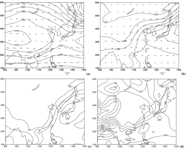
LOVECLIM admittedly exhibits serious weaknesses in its simulation of Asian precipitation. In particular, the sum-mer precipitation is clearly underestimated and the low-level geopotential ridge over the North Pacific is shifted northward 10 degrees in latitude compared to observations (Fig. 1). These weaknesses are most likely caused by insufficient spa-tial resolution and simplified convective physics. As a conse-quence, quantitative estimates of the effects of astronomical parameters and ice sheets on East Asian precipitation should not be interpreted too rigidly. Yet, we believe that LOVE-CLIM has proved to be a reasonably appropriate tool to iden-tify teleconnections. Along with its computing efficiency, this justifies using this model for a first qualitative assess-ment of the connections between ice sheets and sub-tropical dynamics by means of a series of sensitivity experiments.
3 Climate forcings and experiment design
According to the deep-sea δ18O records, MIS-13 is char-acterized by 3 peaks: 13.11, 13.13 and 13.3 (Imbrie et al., 1984; Bassinot et al., 1994; Tiedemann et al., 1994; Shack-leton, 2000; Lisiecki and Raymo, 2005). They occur respec-tively at about 482, 501 and 524 ka BP with dating uncer-tainty of the order of a few thousands of years. For example, MIS13.3 was assumed to peak at 524 ka BP as a compromise between the records of Lisiecki and Raymo (2005), Tiede-mann et al. (1994), Bassinot et al. (1994), Shackleton (2000) and SPECMAP (Imbrie et al., 1984, provided their label 14.0 is changed into 13.3).
In our experiments, the model is forced by (i) the latitu-dinal and seasonal distributions of the energy received from the Sun and computed from the appropriate astronomical el-ements (Berger, 1978), (ii) the GHG concentration retrieved from the Dome C ice core in Antarctica and (iii) the ice sheets assumed to exist during this interglacial. All the climatic fea-tures of the MIS-13 simulations will be compared to the sim-ulated Pre-Industrial (PrI) climate.
3.1 Astronomical and GHG forcings
MIS-13.1 spans a full precession cycle: perihelion oc-curred in NH summer at 485 ka BP (̟ =268.25◦, e=0.03857,
ε=23.212◦), then in winter at 495 ka BP (̟ =97.82◦) and
in summer again at 506 ka BP (̟ =274.05◦). The model
(a) (b)
(c) (d)
Fig. 1. Present-day climate simulated by LOVECLIM. (a) January 850 hPa geopotential height (m) and wind (m/s), (b) July 850 hPa
geopotential height (m) and wind (m/s), (c) January precipitation (cm/year) and (d) July precipitation (cm/year).
506 ka BP, but not for 485 ka BP given that it is very similar to 506 ka BP. Note that the isotopic signals of MIS-13.11 and MIS-13.13 peaked a few thousand years later than 485 ka BP and 506 ka BP, respectively, which is not surprising given the response time of ice sheets. However, we used the extremes of the precession cycle because we are interested in monsoon and the latter is expected to be primarily controlled by pre-cession.
As the strong EASM extends over MIS-13.3 also, it was decided to include this other peak of interglacial MIS-13 in our simulations. Although the ice volume minimum is in fact situated around 524 ka BP, we have adopted the conservative strategy of coupling the minimum ice volume with maxi-mum summer insolation and therefore have chosen a date of 529 ka BP for the MIS-13.3 experiment as it corresponds
to the summer solstice at perihelion (Exp. 8 and Exp. 9 in Table 1).
Being given the revised time scale of EPICA in Jouzel et al. (2007) and the CO2, CH4and N2O concentration given in
Siegenthal et et al. (2005) and Spahni et al. (2005), it was de-cided to use the same GHG concentration both for 506 and 495 ka BP MIS-13.1 experiments (Exp. 2 to Exp. 7 in Ta-ble 1). This hypothesis seems acceptaTa-ble because the GHG values for these two dates are not much different, and aver-ages over that period were used. Taking the same values for the whole MIS-13.1 makes it easier also to test the sensitiv-ity of the climate model to the astronomical forcing alone, in particular to precession.
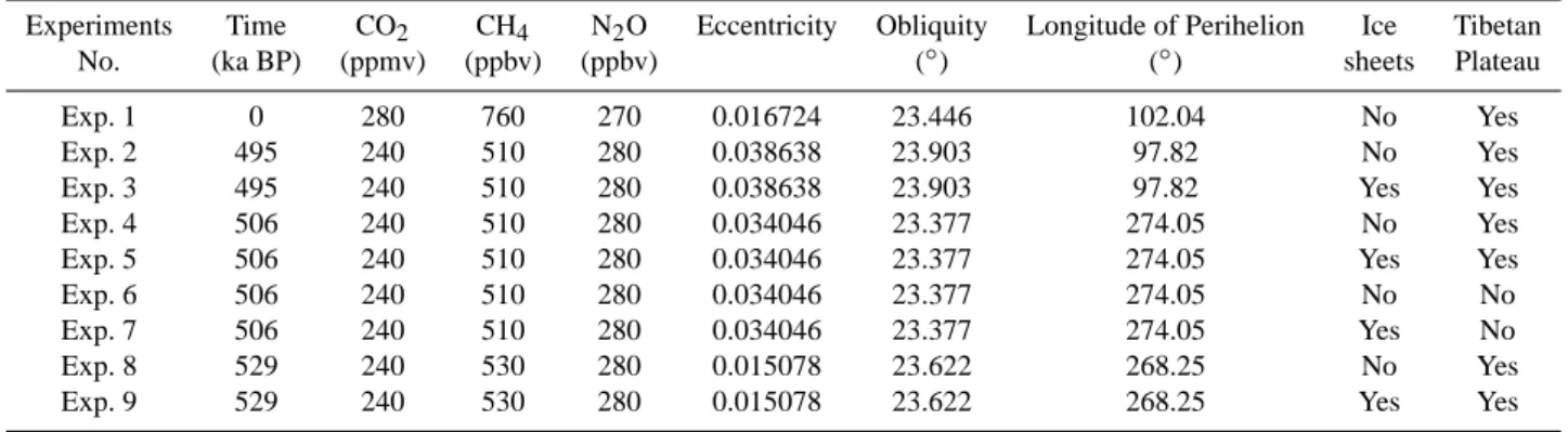
Table 1. The forcings for the different simulations. In this table, 0 ka BP is for Pre-Industrial time, and its greenhouse gases concentration
values are used in the Paleoclimate Modeling Intercomparison Project (Braconnot et al., 2007). Ice sheets means North American and Eurasian ice sheets.
Experiments Time CO2 CH4 N2O Eccentricity Obliquity Longitude of Perihelion Ice Tibetan
No. (ka BP) (ppmv) (ppbv) (ppbv) (◦) (◦) sheets Plateau
Exp. 1 0 280 760 270 0.016724 23.446 102.04 No Yes
Exp. 2 495 240 510 280 0.038638 23.903 97.82 No Yes
Exp. 3 495 240 510 280 0.038638 23.903 97.82 Yes Yes Exp. 4 506 240 510 280 0.034046 23.377 274.05 No Yes Exp. 5 506 240 510 280 0.034046 23.377 274.05 Yes Yes
Exp. 6 506 240 510 280 0.034046 23.377 274.05 No No
Exp. 7 506 240 510 280 0.034046 23.377 274.05 Yes No Exp. 8 529 240 530 280 0.015078 23.622 268.25 No Yes Exp. 9 529 240 530 280 0.015078 23.622 268.25 Yes Yes
3.2 North American (NA) and Eurasian (EA) ice sheets The Greenland and Antarctica ice sheets were kept the same as for the present-day in all the simulations (the present-day ice volume is about 2.9×10⁶km3 for Greenland ice sheet and 24.7×10⁶km3 for Antarctica ice sheet (IPCC, 2007)).
δ18O of deep-sea cores clearly suggest the existence of other ice sheets in the Northern Hemisphere during MIS-13, but it is unfortunately difficult to assess their exact area and vol-umes. The latter were therefore estimated by extrapolat-ing the information available from their LGM reconstruc-tion using δ18O – ice volume – sea level generic relation-ships. We hypothesize that the LGM total ice volume for both NA and EA was 39×106km3, a mid-range value esti-mated from Hughes et al. (1981), Peltier (1994, 1998, 2004), Clark and Mix (2002), Lambeck et al. (2002), and Bintanja et al. (2005). This value is actually pretty close to the ICE-4G (Peltier, 1994) LGM reconstruction (36.1×10⁶km3). The
ra-tio between the excess of ice at the LGM compared to today and that at MIS-13.1 is estimated from the δ18O taken from Imbrie et al. (1984). This leads an ice volume of 11×106km3 of ice at MIS-13.1 and 16.6×10⁶km3of ice at MIS-13.3 to be distributed between NA and EA. We can either assume the ratio between NA and EA was the same as at the LGM (NA is about twice EA in the LGM scenario) or follow Bintanja et al.’s (2005) reconstruction (EA is about twice NA in the Bintanja scenario).
For MIS 13.1, this strategy leads to an ice volume of 7.3 and 3.7×10⁶km3 for respectively NA and EA in the LGM scenario or to 3.7 and 7.3×10⁶km3 in the Bintanja sce-nario. Other reconstructions were calculated based on the
δ18O values of Bassinot et al. (1994), Lisiecki and Raymo (2005), Shackleton (2000) and Tiedemann et al. (1994). Us-ing the LGM reconstruction of the NA and EA ice sheet vol-umes from Peltier (1994) as a reference for the proportion-ality rule leads to MIS-13.1 ice volumes ranging from 1.06 to 4.14×10⁶km3 for EA and from 2.15 to 8.42×10⁶km3
for NA. Corresponding sensitivity studies will be published elsewhere but we anticipate in saying that the conclusions reached in the present paper are qualitatively insensitive to the details of the adopted reconstruction.
Ice sheets are assumed to be axi-symmetric. For a given maximum thickness, h, and a diameter of the circular basis at the ground, l, the volume of such ice sheet is
V = 2πhl2/15 (1)
The thickness of the ice sheet at each grid point can be calculated assuming that we know the relationship between
h and l and the location of the ice sheet centre.
As a first approximation, the relationship between h and l can be estimated from the shape and size of the ice sheets at the LGM. At MIS-13.1, the diameter of NA is about 2600 km and the altitude of its crest above the ground about 1700 m. For EA, these values are roughly 2000 km and 1480 m. At MIS-13.3, these are for NA, 2980 km and 1985 m respec-tively and for EA 2280 km and 1690 m. These values were used in the present paper but we note that according to a theoretical model by Paterson (1994) l is proportional to h2, which leads to slightly different ice sheets properties. Again, these details do not qualitatively affect our conclusions.
Finally, the locations of NA and EA were based on what we know from the initiation of the ice sheets at the last glacial inception (Clark et al., 1993; Bintanja et al., 2002; Peltier, 2004). For NA, we assumed that its center was at (90◦W,
69◦N) and for EA, (50◦E, 63◦N). Simulations were also
made assuming EA is located over Scandinavia (centered at 28◦E, 63◦N). Although these are interesting features to
be discussed in relationship with this change in location, the main conclusions remain again unchanged.
In summary, we will discuss eight experiments (Table 1). Three of them (Exp. 2, 4 and 8) allow to isolate the ef-fect of changing only the astronomical parameters: they are made respectively for 495, 506 and 529 ka BP. Three others (Exp. 3, 5 and 9) test the effect of the ice sheets themselves.
Table 2. Globally averaged surface temperature and precipitation over East China for the 495, 506 and 529 ka BP experiments. All the values
are relative to the simulated Pre-Industrial ones.
Experiments Global Surface temperature (◦C) Precipitation over East China (%)
January July Annual January July Annual
Exp. 2 −0.08 −0.99 −0.41 0 −16 −5
Exp. 4 −1.07 0.84 −0.18 −5 32 7
Exp. 5 −1.7 0.58 −0.64 −15 37 2
Exp. 8 −0.75 0.46 −0.18 −5 18 4
Exp. 9 −1.47 0.04 −0.75 −10 21 −4
They are made for the the same time slices which will there-fore allow them to be compared with Exp. 2, 4 and 8. The last two experiments (Exp. 6 and 7) concern the sensitivity to the Tibetan Plateau at 506 ka BP. Comparing experiments 7 (with ice sheets) and 6 (without ice sheets) shows the im-pact of the ice sheets in absence of the Tibetan Plateau. This will in turn be compared to the difference between experi-ments 5 and 4, a difference which shows the effect of the ice sheets in presence of the Tibetan Plateau. All the experiments are 2000-year long simulations and the climate averages are computed over the last 100 years.
4 Climate response at 495 and 506 ka BP (MIS-13.1)
Table 2 summarizes the global surface temperature and July precipitation over East China simulated for MIS-13.1 and 13.3 (East China is defined as a region from 100 to 120◦E
and 20 to 40◦N, including 25 grids points of LOVECLIM
with an area of 4.3×10⁶km2). 506 ka BP (Northern
Hemi-sphere summer at perihelion, Exp. 4) is globally warmer than 495 (Southern Hemisphere summer at perihelion, Exp. 2), both in July and in annual mean. This result is consis-tent with other experiments we have made (not shown here) where we tested the effect of changing the precession phase by 180◦. It underlines the importance of the Northern
Hemi-sphere response and associated feedbacks at the global scale. Besides this increase in temperature, astronomical situations with summer at perihelion are also associated with a stronger EASM. In July, the precipitation over East China increases by 32% at 506 ka BP (Exp. 4, Table 2) as compared to Pre-Industrial one, but it decreases by 16% at 495 ka BP (Exp. 2). This means that there is far more precipitation in July over East China at 506 ka BP than at 495 ka BP owing to the en-hanced seasonal contrast (Table 2). Actually, this is also true for the regions affected by the African and the In-dian monsoon. For example, precipitation increases by 60% at 506 ka BP as compared to Pre-Industrial one over North Africa (0–30◦N, 20◦W–60◦E), whereas it decreases by 20%
at 495 kyr BP. Over India (10–27◦N, 70–90◦E), these
num-bers are respectively +29% and −10%. So far these results essentially provide a further confirmation of the common
un-derstanding of the effect of precession on temperature and monsoon precipitation.
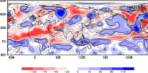
By contrast, the further reinforcement of EASM precipita-tion in response to the introducprecipita-tion of ice sheets (Exp. 5) is surprising because one could think that the continental cool-ing associated with the ice sheets is unfavorable to monsoon dynamics. The July precipitation anomaly resulting from the introduction of ice sheets at 506 ka BP is shown on Figs. 2 (global) and 3a (East Asia). These are differences between Exp. 5 (with ice sheets) and Exp. 4 (without ice sheets). Also shown is the statistical significance (at both the 95% and 99.9% confidence levels) of the anomalies using a Stu-dent t-test. The introduction of ice sheets causes a decrease in precipitation over a band extending from North Africa to Saudi Arabia continuing to the Western Siberian Lowlands, and also over northeastern China and most of Japan (Fig. 2). By contrast, precipitation increases over most of the western part of the Indian subcontinent and over the east of the Ara-bian Sea. More important for our purpose, two main bands with increased rainfall are clearly seen over East Asia. One is south of 35◦N, extending from the eastern margin of the
Ti-betan Plateau through South China and South Japan and dis-appearing over the Pacific Ocean. In this belt, precipitation increases from a few percent to 30% (in qualitative agree-ment with proxy data, e.g. Guo et al., 1998; Yin and Guo, 2006, 2008). This region extends over about 1200 km in lati-tude and 4200 km in longilati-tude and it includes 24 grid points in LOVECLIM (the resolution of which is about 5.6◦
×5.6◦).
The other band extends from the northern margin of the Ti-betan Plateau, through the northwest of China and Mongo-lia, and finally to the north of Lake Baikal. This effect of the ice sheets on the East Asian precipitation is much larger than the interdecadal variability. All precipitation changes greater than roughly 10 cm/year are significant at the 95% confidence level at least. In particular, the center part of the anomalies associated with the wave train discussed here be-low is significant at 99% confidence level. Similar confi-dence levels are reached in all other experiments, like those where the size of the ice sheets is reduced or increased by a factor of two, and those where the center of the Eurasian ice sheet is moved westward 1000 km to be placed finally over
Fig. 2. July precipitation difference between Exp. 5 (with ice sheets) and Exp. 4 (without ice sheets). The color shading indicates precipitation
anomaly in cm/year and the contour lines limit the regions where the anomalies are significant at the 95% and 99.9% confidence levels.
(a) (b)
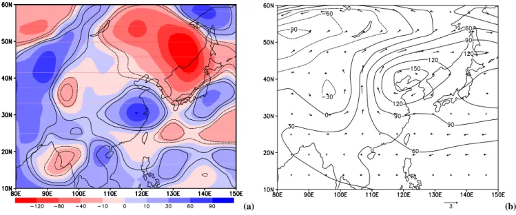
Fig. 3. Exp. 5 minus Exp. 4 for (a) July precipitation (cm/year) and (b) July geopotential (m2s−2) and wind (m/s) at 800 hPa level. In (a)
color shading and contour lines of confidence levels are like in Fig. 2.
Scandinavia (see here below remarks about the impact of the size and geographical location of the Eurasian ice sheet). This precipitation anomaly pattern is also robust on using an-other 100-yr time sampling of the model output time series.
It is also significant that the pressure gradient between the ocean and the continent gets larger when the ice sheets are introduced (Fig. 3b). High geopotential over the ocean be-comes larger and low geopotential deepens over land. The gradient between the ocean and the continent increases by 10–15% from the “no ice sheet” (Exp. 4) to the “with ice sheets” (Exp. 5) experiment. Consistently, we observe a reinforcement of the easterlies blowing from the ocean to the continent, an enhanced convergence and more convec-tive precipitation over East China. Along the coast of
South-East China, the wind velocity increases by 10 to 20% and becomes definitely more easterly. At the same time, the west-erly component of the wind over the continent (blowing to-wards the ocean) intensifies, and convergence over central China increases, which is normally expected to favor precip-itation. In particular, the water vapor flux from the ocean to the continent is seen to increase (by 26% at 124◦E–30◦N for
example) mainly in response to the increase in the easterly wind (from 1.6 to 2.1 ms−1). An analysis of the water budget
in the main center of precipitation increase (∼118◦E–30◦N)
further reveals that the precipitation change is due for 58% to the evaporation change and 42% to change in the divergence of the water vapor flux.
Fig. 4. (a) Upper, difference for July 650-hPa-level omega field (in 0.001 Pa/s) between Exp. 5 (with ice sheets) and Exp. 4 (without ice
sheets); (b) Middle, same as (a) but for January; (c) Lower, difference for July 650-hPa-level omega field (Pa/1000s) between Exp. 7 (with ice sheets) and Exp. 6 (without ice sheets) in the absence of Tibetan Plateau.
While a reinforcement of the summer monsoon with the Northern Hemisphere summer occurring at perihelion was expected, the reinforcement caused by the ice sheets is harder to figure out. The difference in July precipitation between the experiment with ice sheets (Exp. 5) and the one without ice sheet (Exp. 4) (Fig. 2) shows that zone of dry anomaly develops to the West of the Eurasian ice sheet. It results from anticyclonic vorticity forced over the upslope region. Conversely, a wet anomaly develops to the East, due to cy-clonic vorticity forced over the downslope region. Both are expected consequences of the principle of conservation of potential vorticity (see, e.g. Holton 1979:87–91). Even more significant is the appearance of a wave train structure
prop-agating south-eastwards starting from the EA ice sheet and ending up over East China with a reinforcement of precipita-tion. This wave train exactly corresponds to the barotropic model results of Grose and Hoskins (1979) where such a wave train is topographically induced. This wave feature is also seen in LOVECLIM in the 650-hPa-level omega field (Fig. 4a), with alternating large scale ascent and subsidence ending up with a reinforcement of the ascent over China.
This wave train is actually a robust feature of LOVECLIM. It appears also with more or less the same intensity, the same direction and the same wavelength in the following experi-ments:
Fig. 5. July precipitation difference between with and without ice sheets experiments where the 506 ka BP ice sheets volumes are assumed
to be the same as they were at the Last Glacial Maximum and the centre of the NA ice sheet is moved one grid point to the south of its LGM position. Color shading and contour lines of confidence levels are like in Fig. 2.
1. other 100-yr long experiments with the same forcing and boundary conditions as used here.
2. an experiment where the size of the EA ice sheet is doubled according to the reconstruction by Bintanja et al. (2005).
3. an experiment using a shape according to the Paterson’s model assuming a perfectly plastic ice.
4. an experiment where the EA ice sheet has been moved westward 1000 km to finally be placed over Scandi-navia. In this case the direction of the wave train changes only very slightly. The wave train continues to end up over East China with more precipitation which therefore does not change our conclusion.
5. an experiment with the same GHG concentration and ice sheets, but with NH winter at perihelion.
As far as the ice sheet size is concerned, sensitivity ex-periments (not illustrated here) show that there is a thresh-old value beyond which the EASM weakens, but only if the center of the NA ice sheet is moved south of its LGM posi-tion. When the sizes of the 506 ka BP ice sheets are over that threshold, the wave-length of the wave train is such that it does not phase lock any more with the EASM. The center of maximum precipitation increase (as compared to the no ice sheets experiment) falls in the Pacific Ocean (Fig. 5). In all cases before reaching this threshold, the results remain more or less the same as discussed here for Fig. 2.
We have so far no clear explanation on why the wave train adjusts such as to reinforce the EASM, in other words, what is the phase-locking mechanism. It may be related to the Pacific Ocean, the Tibetan Plateau and/or the thermal low over East Asia. In favor of the last possibility though, we
find that in January (Fig. 4b), there is a wave train in the omega field like in July, but it is ending this time with a large scale subsidence which reinforces the winter thermal High over China. We also performed experiments where Tibetan Plateau was removed. Comparing again the experiments with (Exp. 7) and without (Exp. 6) ice sheets in the absence of the Tibetan Plateau, the wave train is still very much present, especially in the omega field at 650 hPa level (Fig. 4c), but with a different wave-length. The ascent previously centered over East China (Fig. 4a) is now over the west Pacific and is replaced by a subsidence (Fig. 4c). This leads to July pre-cipitation over East China being 7% less in Exp. 7 than in Exp. 6. In this case, we would tentatively conclude that the EA ice sheet reinforces the summer precipitation over East China only through the influence of the Tibetan Plateau, the latter being instrumental in shaping the configuration of the wave train.
The existence of the wave train is justified by the barotropic and baroclinic theories summarized by Grose and Hoskins (1979) and Hoskins and Karoly (1981). However, we appreciate that the particular configuration that it adopts in the LOVECLIM model could be model dependent. This will be tested by further investigating with other climate models the mechanisms by which this wave is generated and phase-locked.
Numerical experiments made for MIS-13.1 show therefore that the precipitation over China associated to the EASM is much stronger when Northern Hemisphere summer is at per-ihelion rather than when Southern Hemisphere summer is at perihelion, and that it gets reinforced again after the ice sheets are introduced. These two reinforcements lead actu-ally to create a monsoon which is stronger at 506 ka BP than at the Pre-Industrial. July precipitation over East China in the experiment 506 ka BP with ice sheets (Exp. 5) increases
(a) (b)
Fig. 6. Exp. 5 (506 ka BP with ice sheets) minus Exp. 1 (Pre-Industrial) for (a) July precipitation (cm/year) and (b) July geopotential (m2s−2)
and wind (m/s) at 800 hPa level. In (a) color shading and contour lines of confidence levels are like in Fig. 2.
by about 37% when compared to the Pre-Industrial one (Ta-ble 2, Fig. 6a). This increase of precipitation over East China is in qualitative agreement with the reconstruction made from the proxy records in China. At the same time, July geopoten-tial increases over the ocean and decreases over the conti-nent (Fig. 6b). This means that the pressure gradient be-tween the ocean and the continent increases, leading to a 20 to 80% increase in the southwesterly and southeasterly wind velocity at the 800 hPa level over China. This leads to an increase of the water vapor flux from the ocean to the conti-nent and to a general strengthening of the East Asian summer monsoon. Besides the evaporation process, the overall influ-ence of the ocean would deserve to be discussed (Ohgaito and Abe-Ouchi, 2007). It would be worth testing the relative contribution of the atmospheric convergence and of the sea surface temperature to the increase of water vapor flux.
5 Climate response at 529 ka BP (MIS-13.3)
We decided to analyze the climate during MIS-13.3 because the proxy records from China show that the strong EASM occurred during the period from about 530 to 480 ka BP (e.g. Kukla et al., 1990; Guo et al., 1998), and also because the extreme monsoon over South Asia and Africa occurred near 525–530 ka BP, which is closer to MIS-13.3 than to MIS-13.1 (Bassinot et al., 1994; Rossignol-Strick et al., 1998).
As discussed earlier in Sect. 3, the peak of MIS-13.3 dates 524 ka BP and the selected astronomical forcing for it is at 529 ka BP. The astronomical situations at 529 and 506 ka BP differ essentially through eccentricity which is much smaller at 529 ka BP (0.015 against 0.034 at 506 ka BP). This means
that at 529 ka BP, the distance of the Earth to the Sun at per-ihelion is larger leading to less energy available in North-ern Hemisphere summer (“cooler” summer), but also to less energy globally averaged over the Earth and the year, W , be-cause W =S0/(1−e2)1/2implies that W is smaller for smaller values of e. This “cooler” Northern Hemisphere summer at 529 ka BP is companied by the Eurasian continent being cooler by 1 to 3◦C relative to 506 ka BP (not shown here), and
by a slightly cooler (0.3◦C) over northern Pacific and slightly
warmer (0.6◦C) over Okhotsk and Bering seas. This reduces
the thermal gradient between the land and the adjacent ocean leading to a weaker summer monsoon at 529 ka BP than at 506 ka BP. Consequently, July precipitation over East China is 11% less at 529 ka BP than at 506 ka BP. There is also less July precipitation over North Africa and India.
At 529 ka BP, when the ice sheets are introduced, the same wave train as at 506 ka BP is observed in the precipitation and omega fields. Actually, all the 529 ka BP regional features are about the same as at 506 ka BP. Although weaker than at 506 ka BP, July precipitation over East China at MIS-13.3 is still 21% more abundant than the Pre-Industrial one (Fig. 7a) and the wind velocity is 10 to 40% larger (Fig. 7b). It is therefore not surprising that the proxy data record a strong EASM during the whole MIS-13. The environment has in-deed been affected already strongly by the early monsoon during MIS-13.3. This first impact has been definitely im-printed in the proxy records and reinforced later during MIS-13.13 and MIS-13.11.
(a) (b)
Fig. 7. Exp. 9 (529 ka BP with ice sheets) minus Exp. 1 (Pre-Industrial) for (a) July precipitation (cm/year) and (b) July geopotential (m2s−2)
and wind (m/s) at 800 hPa level. In (a) color shading and contour lines of confidence levels are like in Fig. 2.
6 Conclusions
For the first time, a series of modelling experiments have been made to understand the palaeo-environmental data showing an exceptionally strong East Asian summer mon-soon occurring during the cool MIS-13 interglacial. The main conclusions, using the LOVECLIM model, underline the major role played by both the astronomical and ice sheet forcings, the last mainly through teleconnection:
1. When the Northern Hemisphere summer occurs at peri-helion, like at both 529 and 506 ka BP, the large seasonal contrast leading to the East Asian summer monsoon is more intense than when Southern Hemisphere summer occurs at perihelion, like at 495 ka BP and Pre-Industrial time.
2. The Eurasian ice sheet (its albedo and topography which was deduced from the δ18O record) further enhances the summer precipitation over East China through a wave train propagating south-eastwards from the Eurasian ice sheet. This wave train ending with a large scale ascent over East China is influenced by the Tibetan Plateau and probably phase locked by the East Asian summer low. A consistent pattern of responses is then observed, made of an increase of the air pressure gradient between the Pacific Ocean and the East Asian continent, an intensifi-cation of the low-level south-easterlies blowing from the ocean and an enhanced precipitation over East China. These preliminary results make sense because they are overall consistent with beta-plane atmosphere dynam-ics theory. However, they still need to be substantiated by other more sophisticated climate models, by further
sensitivity analyses to the volume and location of the ice sheets and to the size of the Tibetan Plateau and by investigation of the wave phase-lock process.
3. The regional features at 529 ka BP are very similar to those at 506 ka BP. It is not surprising that the proxy data record a strong EASM during the whole MIS-13. In summary, although the model simulates a situation at 506 and 529 ka BP which is globally cooler than at Pre-Industrial time due to the ice sheets and a lower greenhouse gases concentration, both the Northern Hemisphere summer at perihelion and the atmospheric wave induced by the Eura-sia ice sheet lead to a stronger monsoon than at Pre-Industrial time. This strong monsoon finally contributes to increase the tree fraction over most of China (not shown here), which within the resolution of the model fits well the paleo-record.
Acknowledgements. Qiuzhen Yin has benefited from a grant of
the Belgium FNRS (Fonds de la Recherche Scientifique) and is now postdoctoral fellow at Universit´e catholique de Louvain in Louvain-la-Neuve. M. Crucifix and H. Goosse are research associates with the FNRS.
References
Bassinot, F. C., Labeyrie, L. D., Vincent, E., Quidelleur, X., Shack-leton, N. J., and Lancelot, Y.: The astronomical theory of climate and the age of the Brunhes-Matuyama magnetic reversal, Earth Planet. Sci. Lett., 126, 91–108, 1994.
Berger, A.: Long-term variations of daily insolation and Quaternary Climatic Changes, J. Atmos. Sci., 35(12), 2362–2367, 1978. Bintanja, R., van de Wal, R. S. W., and Oerlemans, J.: Modelled
at-mospheric temperatures and global sea level over the past million years, Nature, 437, 125–128, 2005.
Bintanja, R., van de Wal, R. S. W., and Oerlemans, J.: Global ice volume variations through the last glacial cycle simulated by a 3-D ice-dynamical model, Quatern. Int., 95–96, 11–23, 2002. Braconnot, P., Otto-Bliesner, B., Harrison, S., Joussaume, S.,
Pe-terschmitt, J.-Y., Abe-Ouchi, A., Crucifix, M., Driesschaert, E., Fichefet, T., Hewitt, C. D., Kageyama, M., Kitoh, A., Laˆın´e, A., Loutre, M.-F., Marti, O., Merkel, U., Ramstein, G., Valdes, P., Weber, S. L., Yu, Y., and Zhao, Y.: Results of PMIP2 coupled simulations of the Mid-Holocene and Last Glacial Maximum – Part 1: experiments and large-scale features, Clim. Past, 3, 261– 277, 2007,
http://www.clim-past.net/3/261/2007/.
Brovkin, V., Ganapolski, A., and Svirezhev, Y.: A continuous climate-vegetation classification for use in climate-biosphere studies, Ecol. Modell., 101, 251–261, 1997.
Chen, F. H., Bloemendal, J., Zhang, P. Z., and Liu, G. X.: An 800 ky proxy record of climate from lake sediments of the Zoige Basin, eastern Tibetan Plateau, Palaeogeogr. Palaeocl., 151, 307–320, 1999.
Clark, P. U. and Mix, A. C. (Eds.): Ice sheets and sea level of the last glacial maximum, Quaternary Sci. Rev., 21(1–3), 1–454, 2002. Clark, P. U., Clague, J. J., Curry, B. B., Dreimanis, A., Hicock, S.
R., Miller, G. H., Berger, G. W., Eyles, N., Lamothe, M., Miller, B. B., Mott, R. J., Oldale, R. N., Stea, R. R., Szabo, J. P., Thor-leifson, L. H., and Vincent, J.-S.: Initiation andd evelopment of the Laurentide and Cordilleran ice sheets following the last inter-glaciation, Quaternary Sci. Rev., 12, 79–114, 1993.
Driesschaert, E., Fichefet, T., Goosse, H., Huybrechts, P., Janssens, I., Mouchet, A., Munhoven, G., Brovkin, V., and Weber, S. L.: Modeling the influence of Greenland ice sheet melt-ing on the Atlantic meridional overturnmelt-ing circulation dur-ing the next millennia, Geophys. Res. Lett., 34, L10707, doi:10.1029/2007GL029516, 2007.
Duplessy, J. C., Roche, D. M., and Kageyama, M.: The Deep Ocean During the Last Interglacial Period, Science, 316, 89–91, 2007. EPICA community members: Eight glacial cycles from an
Antarc-tic ice core, Nature, 429, 623–628, 2004.
Gingele, F. X. and Schmieder, F.: Anomalous South Atlantic lithologies confirm global scale of unusual mid-Pleistocene cli-mate excursion, Earth Planet. Sci. Lett., 186, 93–101, 2001. Goosse, H. and Fichefet, T.: Importance of ice-ocean interactions
for the global ocean circulation: a model study, J. Geophys. Res., 104(C10), 23 337–23 355, 1999.
Grose, W. L. and Hoskins, B. J.: On the Influence of Orography on Large-Scale Atmospheric Flow, J. Atmos. Sci., 36, 223–234, 1979.
Guo, Z. T., Liu, T. S., Fedoroff, N., Wei, L. Y., Ding, Z. L., Wu, N. Q., L¨u, H. Y., Jiang, W. Y., and An, Z. S.: Climate extremes in Loess of China coupled with the strength of Deep-Water
Forma-tion in the North Atlantic, Global Planet. Change, 18, 113–128, 1998.
Harris, S. E. and Mix, A. C.: Pleistocene precipitation Balance in the Amazon Basin recorded in deep sea sediments, Quaternary Res., 51, 14–26, 1999.
Holton, J. R.: An introduction to dynamic meteorology, Academic Press, New York, 391 pp., 1979.
Hoskins, B. J. and Karoly, D. J.: The steady linear response of a spherical atmosphere to thermal and orographic forcing, J. At-mos. Sci., 38, 1179–1196, 1981.
Hughes, T. J., Denton, G. H., Andersen, B. G., Schilling, D. H., Fastook, J. L., and Lingle, C. S.: The last great ice sheets: A global view, in: The last great ice sheets, edited by: Denton, G. H. and Hughes, T. J., J. Wiley & Sons, New York, 263–317, 1981.
Imbrie, J., Hays, J. D., Martinson, D. G., McIntyre, A., Mix, A. C., Morley, J. J., Pisias, N. G., Prell, W. L., and Shackleton, N. J.: The orbital theory of Pleistocene climate: support from a revised chronology of the marine δ18O record, in: Milankovitch and Cli-mate, Part 1, edited by: Berger, A. L., Imbrie, J., Hays, J., et al., D. Reidel Pub. Co., 269–305, 1984.
IPCC-Group I: Climate Change 2007: the Physical Science Basis, Summary for Policymakers. Contribution of Working Group I to the Fourth Assessment Report of IPCC, IPCC secretariat, C/O WMO, Geneva, February, 2007.
Joussaume, S., Taylor, K. E., Braconnot, P., Mitchell, J. F. B., Kutzbach, J. E., Harrison, S. P., Prentice, I. C., Broccoli, A. J., Abe-Ouchi, A., Bartlein, P. J., Bonfils, C., Dong, B., Guiot, J., Herterich, K., Hewitt, C. D., Jolly, D., Kim, J. W., Kislov, A., Ki-toh, A., Loutre, M. F., Masson, V., McAvaney, B., McFarlane, N., de Noblet, N., Peltier, W. R., Peterschmitt, J. Y., Pollard, D., Rind, D., Royer, J. F., Schlesinger, M. E., Syktus, J., Thomp-son, S., Valdes, P., Vettorett, G., Webb, R. S., and Wyputta, U.: Monsoon changes for 6000 years ago: Results of 18 simula-tions from the Paleoclimate Modeling Intercomparison Project (PMIP), Geophys. Res. Lett., 26, 859–862, 1999.
Jouzel, J., Masson-Delmotte, V., Cattani, O., Dreyfus, G., Falourd, S., Hoffmann, G., Minster, B., Nouet, J., Barnola, J. M., Chap-pellaz, J., Fischer, H., Gallet, J. C., Johnsen, S., Leuenberger, M., Loulergue, L., Luethi, D., Oerter, H., Parrenin, F., Raisbeck, G., Raynaud, D., Schilt, A., Schwander, J., Selmo, E., Souchez, R., Spahni, R., Stauffer, B., Steffensen, J. P., Stenni, B., Stocker, T. F., Tison, J. L., Werner, M., and Wolff, E. W.: Orbital and Mil-lennial Antarctic Climate Variability over the Past 800,000 Years, Science, 317, 793–796, 2007.
Kukla, G., An Z. S., Melice, J. L., Gavin, J., and Xiao, J. L.: Mag-netic susceptibility record of Chinese Loess, Trans. R. Soc. Ed-inb. Earth Sci., 81, 263–288, 1990.
Kutzbach, E. J. and Guetter, P. J.: The sensitivity of monsoon climates to orbital parameter changes for 9 000 years BP: ex-periments with the NCAR general circulation model, in: Mi-lankovitch and Climate, Part 2, edited by: Berger, A. L., Imbrie, J., Hays, J., et al., D. Reidel Pub. Co., 801–820, 1984.
Lambeck, K., Esat, T. M., and Potter, E. K.: Links between climate and sea levels for the past three million years, Nature, 419, 199– 206, 2002.
Lisiecki, L. E. and Raymo, M. E.: A Pliocene-Pleistocene stack of 57 globally distributed benthic delta δ18O records, Paleoceanog-raphy, 20(1), PA1003; doi:10.1029/2004PA001071, 2005.
Masson, V., Braconnot, P., Jouzel, J., de Noblet, N., Cheddadi, R., and Marchal, O.: Simulation of intense monsoons under glacial conditions, Geophys. Res. Lett., 27, 1747–1750, 2000.
Ohgaito, R. and Abe-Ouchi, A.: The role of ocean thermodynam-ics and dynamthermodynam-ics in Asian summer monsoon changes during the mid-Holocene, Clim. Dynam., 29, 39–50, 2007.
Opsteegh, J. D., Haarsma, R. J., Selten, F. M., and Kattenberg, A.: ECBILT: A dynamic alternative to mixed boundary conditions in ocean models, Tellus, 50A, 348–367, 1998.
Paterson, W. S. B.: The Physics of Glaciers, Pergamon, Tarrytown, N.Y., 1984.
Peltier, W. R.: “Implicit ice” in the global theory of glacial isostatic adjustment, Geophys. Res. Lett., 25(21), 3955–3958, 1998. Peltier, W. R.: Ice age paleotopography, Science, 265, 195–201,
1994.
Peltier, W. R.: Global glacial isostasy and the surface of the ice-age Earth: the ICE-5G (VM2) model and GRACE, Ann. Rev. Earth Planet Sci., 32, 111–149, 2004.
Prell, W. L. and Kutzbach, J. E.: Monsoon variability over the past 150,000 years, J. Geophys. Res., 92, 8411–8425, 1987. Prokopenko, A. A., Williams, D. F., Kuzmin, M. L., Karabanov, E.
B., Khursevich, G., and Peck, J. A.: Muted climate variations in continental Siberia during the mid-Pleistocene epoch, Nature, 418, 65–68, 2002.
Renssen, H., Goosse, H., and Fichefet, T.: Modeling the effect of freshwater pulses on the early Holocene climate : The influence of high-frequency climate variability, Paleoceanography, 17(2), 1020, doi:10.1029/2001PA000649, 2002.
Roche, D. M., Dokken, T. M., Goosse, H., Renssen, H., and We-ber, S. L.: Climate of the last glacial maximum: sensitivity stud-ies and model-data comparison with the LOVECLIM coupled model, Clim. Past, 3, 205–224, 2007,
http://www.clim-past.net/3/205/2007/.
Rossignol-Strick, M., Paterne, M., Bassinot, F. C., Emeis, K.-C., and De Lange, G. J.: An unusual mid-Pleistocene monsoon pe-riod over Africa and Asia, Nature, 392, 269–272, 1998. Shackleton, N. J.: The 100,000-year Ice-Age Cycle identified and
found to lag temperature, carbon dioxide and orbital eccentricity, Science, 289, 1897–1902, 2000.
Siegenthaler, U., Stocker, T. F., Monnin, E., L¨uthi, D., Schwander, J., Stauffer, B., Raynaud, D., Barnola, J.-M., Ficher, H., Masson-Delmott, V. and Jouzel, J.: Stable carbon cycle-climate relation-ship during the late Pleistocene, Science, 310, 1313–1317, 2005. Schmieder, F., Dobeneck, T., and Bleil, U.: The Mid-Pleistocene climate transition as documented in the deep South Atlantic Ocean: initiation, interim state and terminal event, Earth Planet. Sci. Lett., 179, 539–549, 2000.
Spahni, R., Chappellaz, J., Stocker, T. F., Loulergue, L., Hausam-mann, G., Kawamura, K., Fluckiger, J., Schwander, J., Raynaud, D., Masson-Delmotte, V., and Jouzel, J.: Atmospheric Methane and Nitrous Oxide of the Late Pleistocene from Antarctic Ice Cores, Science, 310, 1317–1321, 2005.
Tiedemann, R., Sarntheim, M., and Shackleton, N. J.: Astronomic timescale for the Pliocene Atlantic δ18O and dust flux records of Ocean Drilling Program site 659, Paleoceanography, 9, 619–638, 1994.
Timmermann A., Justino Barbosa, F., Jin, F. F., and Goosse, H.: Surface temperature control in the North Pacific during the last glacial maximum, Clim. Dynam., 23, 353–370, 2004.
Wang, B., Clemens, S. C., and Liu, P.: Contrasting the Indian and East Asian monsoons: implications on geologic timescales, Mar. Geol., 201, 5–21, 2003.
Wang, P., Tian, J., Cheng, X., Liu, C., and Xu, J.: Major Pleistocene stages in a carbon perspective: The South China Sea record and its global comparison, Paleoceanography, 19, PA4005, doi:10.1029/2003PA000991, 2004.
Yanase, W. and Abe-Ouchi, A.: The LGM surface climate and at-mospheric circulation over East Asia and the North Pacific in the PMIP2 coupled model simulations, Clim. Past, 3, 439–451, 2007,
http://www.clim-past.net/3/439/2007/.
Yin, Q. Z. and Guo, Z. T.: Mid-Pleistocene vermiculated red soils in southern China as an indication of unusually strengthened East Asian monsoon, Chinese Sci. Bull., 51(2), 213–220, 2006. Yin, Q. Z. and Guo, Z. T.: Strong summer monsoon during the cool
MIS-13, Clim. Past, 4, 29–34, 2008, http://www.clim-past.net/4/29/2008/.


![[PDF] Cours C++ Saisie de nombres et de caractères au clavier | Cours informatique](data:image/gif;base64,R0lGODlhAQABAIAAAP///wAAACH5BAEAAAAALAAAAAABAAEAAAICRAEAOw==)