HAL Id: hal-00296039
https://hal.archives-ouvertes.fr/hal-00296039
Submitted on 28 Sep 2006
HAL is a multi-disciplinary open access
archive for the deposit and dissemination of
sci-entific research documents, whether they are
pub-lished or not. The documents may come from
teaching and research institutions in France or
abroad, or from public or private research centers.
L’archive ouverte pluridisciplinaire HAL, est
destinée au dépôt et à la diffusion de documents
scientifiques de niveau recherche, publiés ou non,
émanant des établissements d’enseignement et de
recherche français ou étrangers, des laboratoires
publics ou privés.
Some aspects of the energy balance closure problem
T. Foken, F. Wimmer, M. Mauder, C. Thomas, C. Liebethal
To cite this version:
T. Foken, F. Wimmer, M. Mauder, C. Thomas, C. Liebethal. Some aspects of the energy balance
closure problem. Atmospheric Chemistry and Physics, European Geosciences Union, 2006, 6 (12),
pp.4395-4402. �hal-00296039�
www.atmos-chem-phys.net/6/4395/2006/ © Author(s) 2006. This work is licensed under a Creative Commons License.
Chemistry
and Physics
Some aspects of the energy balance closure problem
T. Foken, F. Wimmer, M. Mauder, C. Thomas, and C. Liebethal
Department of Micrometeorology, University of Bayreuth, 95440 Bayreuth, Germany Received: 23 November 2005 – Published in Atmos. Chem. Phys. Discuss.: 27 April 2006 Revised: 20 July 2006 – Accepted: 21 September 2006 – Published: 28 September 2006
Abstract. After briefly discussing several reasons for the
energy balance closure problem in the surface layer, the pa-per focuses on the influence of the low frequency part of the turbulence spectrum on the residual. Changes in the tur-bulent fluxes in this part of the turbulence spectrum were found to have a significant influence on the changes of the
residual. Using the ogive method, it was found that the
eddy-covariance method underestimates turbulent fluxes in the case of ogives converging for measuring times longer than the typical averaging interval of 30 min. Additionally, the eddy-covariance method underestimates turbulent fluxes for maximal ogive functions within the averaging interval, both mainly due to advection and non-steady state condi-tions. This has a considerable influence on the use of the eddy-covariance method.
1 Introduction
During the late 1980s it became obvious that the energy bal-ance at the earth’s surface could not be closed with exper-imental data. The available energy, i.e. the sum of the net radiation and the ground heat flux, was found in most cases to be larger than the sum of the turbulent fluxes of sensible and latent heat. This was a main topic of a workshop held in 1994 in Grenoble (Foken and Oncley, 1995). In most of the land surface experiments (Bolle et al., 1993; Kanemasu et al., 1992; Tsvang et al., 1991), and also in the carbon diox-ide flux networks (Aubinet et al., 2000; Wilson et al., 2002), a closure of the energy balance of approximately 80% was found. The residual is
Res = Rn−H − λE − G (1)
with Rn: net radiation, H : sensible heat flux, λE: latent heat flux, and G: soil heat flux. The problem cannot be described
Correspondence to: T. Foken
(thomas.foken@uni-bayreuth.de)
only as an effect of statistically distributed measuring errors because of the clear underestimation of turbulent fluxes or overestimation of the available energy. In the literature, sev-eral reasons for this incongruity have been discussed, most recently in an overview paper by Culf et al. (2004):
i) The most common point of discussion were measure-ment errors, especially those of the eddy-covariance technique, which cause a systematic underestimation of the turbulent fluxes. Improvements in the sensors, in the correction methods and the application of a more stringent determination of the data quality (Foken et al., 2004) have made this method much more reliable in the past ten years (Moncrieff, 2004).
ii) Because of different balance layers and scales of diverse measuring methods (net radiation – surface, turbulent fluxes – approx. 5 m above the surface, and soil heat flux – approx. 10 cm below the surface), the energy storage in the canopy and the soil was often discussed as a rea-son for the unclosed energy balance. Foken et al. (2001) reported for the total solar eclipse over Europe in 1999 that there is a time shift between the irradiation and the turbulent fluxes of up to 30 min, which has an influence on the energy balance closure. Kukharets et al. (2000) also found that the soil heat flux and the energy balance closure are closely related due to the energy storage in the upper soil layer. For an exact determination of the soil heat flux, including storage effects, the energy bal-ance was shown to be closed at night for non-turbulent conditions (Mauder et al., 2006). The storage in the canopy is often negligible.
iii) The unclosure of the energy balance was also connected with the heterogeneity of the land surface (Panin et al., 1998). The authors assumed that the heterogeneities generate eddies at larger time scales than eddies mea-sured with the eddy-covariance method. This problem
4396 T. Foken et al.: The energy balance closure problem is also closely connected with advection and fluxes due
to longer wavelengths (Finnigan et al., 2003; Sakai et al., 2001) or organized turbulence structures (Inagaki et al., 2006; Kanda et al., 2004).
This study is based on a selected data set of the LITFASS-2003 experiment (Mengelkamp et al., 2006) and focuses on the last question (iii) of the closure problem. It is assumed that the problems related to questions (i) and (ii) were ver-ified and corrected according to our present knowledge for the data set used by Mauder et al. (2006). The present study investigates single time series for a selected data set instead of the presentation of daily cycles and sums of the residual of the energy balance closure as done by Mauder et al. (2006) for the LITFASS-2003 experiment.
2 Selected data set of the LITFASS-2003 experiment
The aim of the LITFASS-2003 experiment in May and June of 2003 was to investigate turbulent fluxes in an heteroge-neous landscape sized as a typical numerical weather and
climate model of 20×20 km2(Beyrich et al., 2002a) in the
region of the Meteorological Observatory Lindenberg of the German Meteorological Service southeast of Berlin, Ger-many. The experimental design was similar to the earlier experiment LITFASS-98 (Beyrich et al., 2002b) with an up-dated und enlarged measuring concept and closer relations to the modelling concept. For this study, only the data set of the University of Bayreuth over a maize field (Z´ea m´ays L.) was selected. It was located near the Boundary-Layer Field
Site of the German Meteorological Service (52◦1000100N,
14◦0702700E, 73 m a.s.l.) at Falkenberg. The field can be
characterized as nearly bare soil at the beginning of the ex-periment and by a canopy height of about 45–55 cm on the selected days of this study with a very low leaf-area index.
For this investigation, a data set of only three days (07– 09/06/2003) was selected, which was characterised by an increasing wind velocity from 07 to 09/06/2003 and nearly ideal and identical daily cycles of irradiation with only some scatter due to clouds on 09/06/2003. The conditions dis-cussed later are not restricted to this period; the selected days are “Golden Days” to explain these results of this study. The results are also compared with the data set of the whole ex-periment from 22/05/2003 to 17/06/2003.
Furthermore, the site was intentionally selected to make use of high quality sensors and the opportunity to study the dynamics of the heat storages in the soil. The turbulence complex (2.69 m above ground) was equipped with a sonic anemometer (CSAT3, Campbell Inc., USA) and a LICOR 7500 gas analyzer (LICOR, USA). The data correction and calculation procedure is described by Mauder and Foken (2004), including a complete quality control and footprint analysis (Foken et al., 2004). Additionally, the radiation sen-sors (albedometer: CM24, Kipp & Zonen, Netherlands; dou-ble dome pyrgeometer: PIR, Eppley, USA) were compared
before the experiment. The soil was equipped with five heat flux plates, a temperature profile with nine levels, and a soil moisture profile with three levels. The soil heat flux at the surface was calculated from a combination of the gradient approach (applied at 20 cm depth) and calorimetry (change in soil heat storage with time, applied between 0 and 20 cm depth), which was found by a sensitivity analysis as an opti-mal approach (Liebethal et al., 2005).
During the measurement period from 19/05/2003 to
17/06/2003, temperature maxima were above 25◦C every
day. Absolute humidity ranged between 5 and 15 g m−3.
Typical maxima of both sensible and latent heat flux ranged
between 150 Wm−2and 200 Wm−2. The average wind
ve-locity was approx. 3 m s−1and 30 min maxima and at 10 m
height were 11 m s−1. The atmospheric stratification
ex-pressed by the dimensionless parameter z/L, where z is the measurement height of 2.69 m and L is the Obukhov length, varied between 0.5 during nighttime and −0.5 during day-time.
3 Investigation of the residual of the energy balance clo-sure
As mentioned in the brief introduction, the reason for the residual of the energy balance closure is probably less con-nected with the high frequency part of the turbulence spectra (i and ii) but with the low frequency part (iii). Therefore in this section, based on the usual averaging interval for turbu-lent fluxes of 30 min, the high and low frequency parts were separately investigated and finally, the low frequency part of the spectra was analysed up to 240 min. This paper only cov-ers the problem of fluxes within a not very large extension of the averaging interval. Longer extensions of the averaging interval, as well as results regarding to the problems I and ii, are discussed in an overview paper about the energy balance closure during LITFASS-2003 (Foken et al., 2006).
3.1 The low and high frequency part of the turbulence
spec-tra
For this investigation, the turbulent time series were split into parts of frequencies lower and higher than 0.1 Hz us-ing a wavelet filter (Thomas and Foken, 2005). Low and high-frequency fluxes were determined by means of eddy-covariance using the filtered data. The method is energy con-sistent, because the sum of both fluxes is equal to the flux determined for the 30 min interval with the eddy-covariance method.
Because a direct comparison of both parts of the turbulent flux with the residual did not show a significant correlation, the temporal dynamics of the fluxes and the residual was in-vestigated. For this purpose both parts of the sensible and latent heat flux and the residual were determined at a tempo-ral resolution of five minutes based on overlapping 30-min
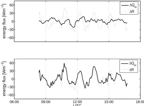
−60 −30 0 30 60 energy flux [Wm −2 ] 06:00 09:00 12:00 15:00 18:00 −60 −30 0 30 60 UTC energy flux [Wm −2 ] ΔQ lo ΔR ΔQ hi ΔR
Fig. 1. Comparison of the change of the turbulent fluxes of sensible and latent heat in the high frequency range (1Qhi)and the low frequency
range (1Qlo)and the change of the residual of the energy balance closure (1R) for 30 min averages determined for time steps of 5 min. A
moving average (daily cycle) was subtracted (08/06/2003).
intervals. The change of each parameter between two adja-cent time stamps was used as a measure of its temporal dy-namics. Subsequently, the correlation between the temporal dynamics and the different flux contributions and the tempo-ral dynamics of the residual was analyzed. In order to reduce the number of parameters to be analysed, the high-frequency part of both sensible and latent heat flux were summed up to
build the high-frequency turbulent heat flux Qhi. The
turbu-lent flux in the low-frequency range Qlo was defined
anal-ogously. Building such composite fluxes is reasonable be-cause the correlation between the dynamics of the two low-frequency parts and accordingly the two high-low-frequency parts
is obvious (R2>0.5), whereas the dynamics of the two parts
of the sensible as well as of the latent heat flux are not corre-lated significantly (R2<0.1).
No correlations were found between the changes of the
tur-bulent fluxes in the high frequency range Qhiand the changes
of the residual. On the contrary, the changes of the
turbu-lent fluxes in the low frequency range Qloand the change of
the residual are closely connected (Fig. 1) and were
signif-icantly correlated on 07/06/2003 (R2=0.85) and 08/06/2003
(R2=0.71). On 09/06/2003 (with changing cumulus
cloudi-ness) no significant correlation was found. A lesser degree of correlation was always associated with steep jumps of the net radiation due to changing cloudiness, because the inertial re-action of the turbulent fluxes leads to a highly variable resid-ual in such situations. Excluding all data with a change in net radiation greater than 2.5 times its standard deviation for
all three days, significant correlations (R2=0.85; 0.89; 0.87)
were found for the low-frequency range, but still not for the high-frequency range.
From these findings it follows that the residual of the en-ergy balance closure is more connected with the low fre-quency part of the turbulent flux than with the high frefre-quency part. In the following section this low frequency part will be investigated with the suitable ogive test.
3.2 The ogive test
Desjardins at al. (1989) and Oncley et al. (1990) introduced the ogive function into the investigation of turbulent fluxes. This function was proposed as a test to check if all low fre-quency parts are included in the turbulent flux measured with the eddy-covariance method (Foken et al., 1995; Foken et al., 2004). The ogive is the cumulative integral of the co-spectrum starting with the highest frequencies
ogw,x(f0) = f0
Z
∞
Cow,x(f ) df (2)
with Cow,x: co-spectrum of a turbulent flux, w: vertical wind
component, x: horizontal wind component or scalar, f : fre-quency. In this study, co-spectra for all interesting combina-tions of time series were calculated up to four hours. Though
only frequency values higher than approx. 1.39 10−4Hz that
correspond to periods of two hours and shorter were used for the test, an underlying interval of four hours improves the statistical significance. Longer periods were not investi-gated due to the daily cycle of the fluxes and high non-steady
4398 T. Foken et al.: The energy balance closure problem
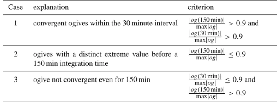
Table 1. Definition of three different cases for the behaviour of ogive functions.
Case explanation criterion
1 convergent ogives within the 30 minute interval |og(150 min)|max|og| >0.9 and
|og(30 min)|
max|og| >0.9
2 ogives with a distinct extreme value before a 150 min integration time
|og(150 min)|
max|og| ≤0.9
3 ogive not convergent even for 150 min |og(30 min)|max|og| ≤0.9 and
|og(150 min)|
max|og| >0.9
state conditions. Because the ogive test must be done with the original not gap-filled time series special tests must be done: The ogive test fails if missing values are in the time series. It was found that even for 288 000 data points (4 h) only intervals without any missing values can be accepted in order to avoid that any ogives based on defective co-spectra are marked as reliable by an automated selection scheme. However, a number of ogives that look quite realistic are dis-carded due to this rigorous criterion. Furthermore, the time shift of the vertical wind and the horizontal wind or scalar in the original data must be below 0.5 s and has to be corrected. The number of acceptable data sets was different for the mo-mentum, sensible and latent heat flux. To compare the data, only data sets acceptable for all three fluxes were analyzed. Therefore the number was reduced to 17 for the Golden Days and 121 for the whole experiment. The convergence of the ogive was analysed as follows:
In the ideal convergent case, the ogive function increases during the integration from high frequencies to low frequen-cies until a certain value is reached and remains on a more or less constant plateau before a 30 min integration time. If this condition is fulfilled, the 30 min covariance is a reliable esti-mate for the turbulent flux, because we can assume that the whole turbulent spectrum is covered within that interval and that there are only negligible flux contributions from longer wavelengths (Case 1). Because of the variability of spec-tra we tolerate deviations of 10% for the plateau value when defining Case 1 (Table 1). Figure 2a can serve as an exam-ple for this case. But it can also occur that the ogive func-tion shows an extreme value and decreases again afterwards (Case 2, Fig. 2b) or that the ogive function doesn’t show a plateau but increases throughout (Case 3, Fig. 2c). Ogive functions corresponding to Case 2 or 3 indicate that a 30 min flux estimate is possibly inadequate.
An overview of the number of measuring series compliant with these cases is given in Table 2 for all three days and the whole experiment. Note that adjacent four hour time series upon which the ogives are based overlap for two hours in order to attain higher temporal resolution. On 09/06/2003,
all acceptable ogives are convergent (Case 1) and most of the time a convergent ogive function was already reached after five minutes for all fluxes. On 07 and 08/06/2003, the ogives for the latent heat flux are more often convergent than the ogives of the sensible heat flux. There is a trend that ogives with a maximum for shorter integration intervals (Case 2) occur on 07/06/2003. Typical differences in the frequency of the cases in the morning and afternoon hours could not be found within the small data set used.
From these findings, it follows that the eddy-covariance method does not measure the total flux within the 30 min in-terval in all cases. The 30 min flux may be reduced because the total flux was already reached in a shorter time period (Case 2) and an integration of up to 30 min reduces the fluxes due to non-steady state conditions or longwave trends, or be-cause significant flux contribution can be found for integra-tion periods larger than 30 min (Case 3).
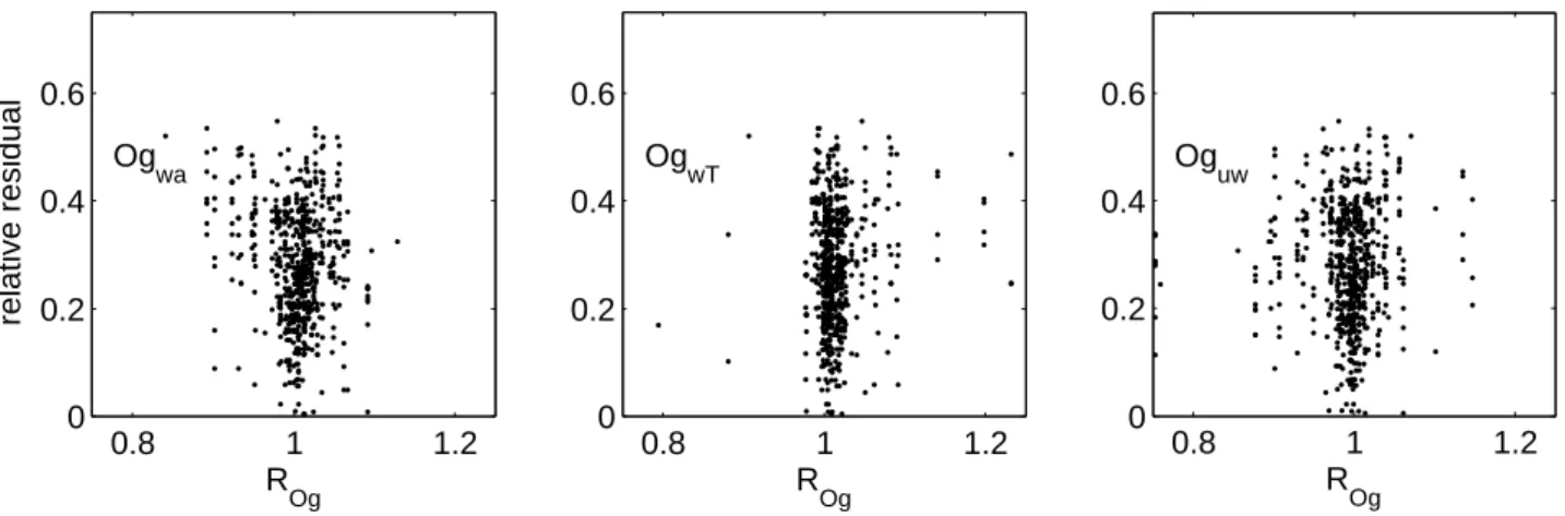
To underline this finding, the relative residual (residual normalised by the available energy)
Res Rn−G
(3) was compared with value of the ogive at 120 min integration time divided by the ogive value with an integration time of 30 min:
Rog =
og120 min
og30 min (4)
This is illustrated in Fig. 3. For Rog∼1, the ogives
con-verge within the 30 min time interval (Case 1). In the case
of a good convergence of the ogives (Rog=1), all values of
the relative residual are possible, including the case that the relative residual less than 0.1 (the energy balance equation is fully closed). For Rog>1 the ogives converge for longer time
intervals than 30 minutes (Case 3) and for Rog<1 they have
a maximum (Case 2), in most cases for time intervals lower than 30 min. In Fig. 3, for high relative residuals the scatter
of Rog is quite high, while low relative residuals correspond
with Rog≈1. A triangle-like structure with the top pointing
downwards can be seen in every subplot. The bottom border
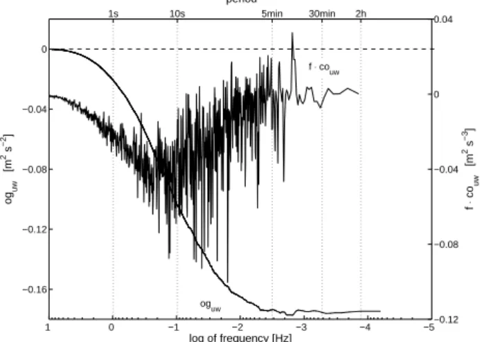
−5 −4 −3 −2 −1 0 1 −0.12 −0.08 −0.04 0 0.04 f ⋅ co uw [m 2 s −3 ] log of frequency [Hz] 2h 30min 5min 10s 1s −0.16 −0.12 −0.08 −0.04 0 og uw [m 2 s −2 ] period f ⋅ couw oguw
Fig. 2a. Ogiven (og) convergent within 30 minutes (Case 1) and
co-spectrum (co), momentum flux on 09/06/2003 (12:30–16:30 UTC).
−5 −4 −3 −2 −1 0 1 −0.05 −0.04 −0.03 −0.02 −0.01 0 0.01 0.02 0.03 f ⋅ co uw [m 2 s −3 ] log of frequency [Hz] 2h 30min 5min 10s 1s −0.035 −0.03 −0.025 −0.02 −0.015 −0.01 −0.005 0 0.005 og uw [m 2 s −2 ] period f ⋅ couw oguw
Fig. 2b. Ogive (og) with a distinct maximal value (extreme) and
a decline for longer integration periods (Case 2) and co-spectrum (co), momentum flux on 07/06/2003 (10:30–14:30 UTC).
of the triangle could be taken as a possible minimum value
of the relative residual at a certain value of Rog. Obviously,
Rog≈1 is a constraint for a possible minimum value of the
relative residual.
It must be assumed that a reduction of the turbulent fluxes also occurs if the ogive function has an extreme value for time periods lower than 30 min and decreases for longer inte-gration times (Case 2). This case occurs only in the transition time with non steady state conditions or in periods with low fluxes. This can be seen from the comparison of the values of the ogive function in Figs. 2a and b. Therefore, this case is not very easy to investigate, because of its infrequent oc-currence. It seems, especially for the sensible heat flux, that different eddy sizes have different signs of the flux as well.
Furthermore, the flux is underestimated in the 30 min inte-gration time if energy is also transported with low frequency eddies (Case 3). Reasons for that are non-steady state
con-−5 −4 −3 −2 −1 0 1 −12 −8 −4 0 4 f ⋅ co uw [m 2 s −3 ] x 10 −3 log of frequency [Hz] 2h 30min 5min 10s 1s −8 −6 −4 −2 0 og uw [m 2 s −2 ] x 10 −3 period f ⋅ couw oguw
Fig. 2c. Ogive (og) not convergent within 30 minutes (Case 3) and co-spectrum (co), momentum flux on 08/06/2003 (02:30– 06:30 UTC).
Table 2. Number of convergent ogives (Case 1), ogives with an
ex-treme value (Case 2), non-convergent ogives (Case 3) for the three investigated days of the ogives of fluxes of momentum (oguw),
sen-sible heat (ogwT), latent heat (ogwa). The data were selected
ac-cording to the data quality given in the text. The numbers in brack-ets are for the whole period from 22/05/2003 to 17/06/2003 with the percentages of the data set of 121 series.
Case 1 Case 2 Case 3
oguw 14 (103, 85%) 2 (13, 11%) 1 (5, 4%)
ogwT 14 (100, 83%) 2 (14, 12%) 1 (7, 6%)
ogwa 16 (100, 83%) 1 (17, 14%) 0 (4, 3%)
ditions and trends, which either cannot entirely or at least not sufficiently be found with the relevant tests (Foken and Wichura, 1996; Vickers and Mahrt, 1997), or advective con-ditions. These findings explain the fact that turbulent fluxes are always underestimated. A simplified correction of the turbulent fluxes by the ratio of the ogive function for 30 min and the maximum ogive function (extreme or convergence) shows a reduced residual (Fig. 4). Because the change of the flux is not very large and relevant only for approx. 80–85% of the data both parts of Fig. 4 (uncorrected and corrected) are not very different. More interesting is the visible result, that the correction has a different influence at different days, mainly for 07/06/2003 and nearly not at all for 09/06/2003. Therefore, the hypothesis given above about the forcing of the fluxes should be a subject of further investigations.
4 Conclusions
From the findings of this study and from many papers it can be assumed that turbulent fluxes in the high frequency
4400 T. Foken et al.: The energy balance closure problem 0.8 1 1.2 0 0.2 0.4 0.6 relative residual R Og 0.8 1 1.2 0 0.2 0.4 0.6 R Og 0.8 1 1.2 0 0.2 0.4 0.6 R Og Og wa OgwT Oguw
Fig. 3. Relative residual (residual normalised with the available energy) dependent on the ratio Rog=og(120 min)/og(30 min) for the sensible
and latent heat flux, and the momentum flux.
00:00 06:00 12:00 18:00 00:00 −200 −100 0 100 residual (original) [Wm −2 ] UTC 00:00 06:00 12:00 18:00 00:00 −200 −100 0 100 residual (corrected) [Wm −2 ] UTC 07/06/2003 08/06/2003 09/06/2003 07/06/2003 08/06/2003 09/06/2003
Fig. 4. Residual of the energy balance closure for 30 min averages: on the left side are the calculations with high quality radiation and flux
data, and on the right side these calculations are corrected for turbulent fluxes by the ratio max |og|/og (30 min).
range of the turbulent spectra can be measured exactly with the eddy-covariance method. All necessary corrections of the high frequency part of the spectra are, according to our present knowledge, well done and cannot explain the resid-ual of the energy balance closure (i). In addition, time shifts between different fluxes due to storage influences cannot ex-plain the residual for 30 min means (ii).
Therefore, the main reasons for the unclosed energy bal-ance are influences on the low frequency part of the turbu-lence spectra (iii) caused by the landscape of the area where the flux measuring site is situated, as already assumed by Finnigan et al. (2003). A possible explanation can be orga-nized turbulent structures (Kanda et al., 2004) or secondary circulations (Inagaki et al., 2006). The turbulent fluxes in the low frequency part of the spectra can influence the flux in two ways and can partly explain the residual of the energy balance closure. One reason, already discussed by Finnigan et al. (2003), are fluxes missing because of a convergence of the ogive function for integration times larger than 30 min
(Case 3). The reduction of the turbulent fluxes in situations when the ogive function has an extreme value for time pe-riods lower than 30 min may also be caused by fluxes in the low frequency part with the opposite sign (Case 2). The ogive function can be helpful to investigate such situations and also to partly correct the energy loss. But the effect of a correc-tion of the fluxes using an ogive funccorrec-tion can only explain the energy balance problem by 5–10% (Foken et al., 2006), which can be seen from Fig. 4.
It is also interesting that on 09/06/2003 the residual of the energy balance closure has its lowest values and the ogive function is often convergent after only five minutes (Fig. 4). The day is characterised by the highest wind velocities of
up to 7 m s−1and a quickly changing irradiation due to
cu-mulus clouds. This may indicate a forcing of the turbulent exchange in time periods of about five minutes. On the other hand, the day with the lowest wind velocities (07/06/2003) also has a reduced residual. This agrees with findings by Jegede et al. (2004) describing an experiment in the tropics
with a strong radiation forcing, where the energy balance was closed in most of the cases. For this experiment, the same data calculation software was used as for LITFASS-2003. Obviously under cases with a strong radiation forcing or with a highly variable radiation and velocity forcing with time pe-riods shorter than 30 min the influence of the landscape and larger turbulent structures discussed above is reduced.
All turbulent fluxes do not have for all conditions a similar convergence of the ogives (Table 2). While a similarity of scalars was found for the high frequency spectra (Pearson Jr. et al., 1998), typical differences were found in the low fre-quency part (Ruppert et al., 2006), probably connected with the sink/source functions of the scalars, which can be dif-ferent during the daily cycle. Therefore, the residual of the energy balance cannot be used for the correction of other tur-bulent fluxes like the carbon dioxide flux and other trace gas fluxes. Each flux must be analysed separately.
Summarising these results, the eddy-covariance method should be used in some cases with a variable integration period, where the length of this period can be determined by the maximum of the ogive function. This implies that the influence of the advection and low frequency turbulence structures can be partially estimated. This paper can only be a first initiative to investigate more carefully the low frequency part of the turbulent fluxes in relation to the energy balance closure problem. Much more data sets under different conditions must be analysed in a similar way to investigate this hypothesis and to create new findings for
the use of the eddy-covariance method. It must also be
mentioned that many correction methods for the eddy-covariance method are based on the high frequency part of the turbulence spectra and cannot simply be transferred for longer integration intervals.
Edited by: A. B. Guenther
References
Aubinet, M., Grelle, A., Ibrom, A., Rannik, ¨U., Moncrieff, J., Fo-ken, T., Kowalski, A. S., Martin, P. H., Berbigier, P., Bernhofer, C., Clement, R., Elbers, J., Granier, A., Gr¨unwald, T., Morgen-stern, K., Pilegaard, K., Rebmann, C., Snijders, W., Valentini, R., and Vesala, T.: Estimates of the annual net carbon and water exchange of forests: The EUROFLUX methodology, Adv. Ecol. Res., 30, 113–175, 2000.
Beyrich, F., Herzog, H.-J., and Neisser, J.: The LITFASS project of DWD and the LITFASS-98 Experiment: The project strategy and the experimental setup, Theor. Appl. Climat., 73, 3–18, 2002a. Beyrich, F., Richter, S. H., Weisensee, U., Kohsiek, W., Lohse, H.,
DeBruin, H. A. R., Foken, T., G¨ockede, M., Berger, F. H., Vogt, R., and Batchvarova, E.: Experimental determination of turbu-lent fluxes over the heterogeneous LITFASS area: Selected re-sults from the LITFASS-98 experiment, Theor. Appl. Climat., 73, 19–34, 2002b.
Bolle, H.-J., Andr´e, J.-C., Arrie, J. L., Barth, H. K., Bessemoulin, P., A., B., DeBruin, H. A. R., Cruces, J., Dugdale, G., Engman, E. T., Evans, D. L., Fantechi, R., Fiedler, F., Van de Griend, A.,
Imeson, A. C., Jochum, A., Kabat, P., Kratsch, P., Lagouarde, J.-P., Langer, I., Llamas, R., Lopes-Baeza, E., Melia Muralles, J., Muniosguren, L. S., Nerry, F., Noilhan, J., Oliver, H. R., Roth, R., Saatchi, S. S., Sanchez Diaz, J., De Santa Olalla, M., Shut-leworth, W. J., Sogaard, H., Stricker, H., Thornes, J., Vauclin, M., and Wickland, D.: EFEDA: European field experiment in a desertification-threatened area, Ann. Geophys., 11, 173–189, 1993,
http://www.ann-geophys.net/11/173/1993/.
Culf, A. D., Foken, T., and Gash, J. H. C.: The energy balance clo-sure problem, in: Vegetation, water, humans and the climate. A new perspective on an interactive system, edited by: Kabat, P., Claussen, M., Dirmeyer, P. A., et al., Springer, Berlin, Heidel-berg, 159–166, 2004.
Desjardins, R. L., MacPherson, J. I., Schuepp, P. H., and Karanja, F.: An evaluation of aircraft flux measurements of CO2, water
vapor and sensible heat., Boundary-Layer Meteorol., 47, 55–69, 1989.
Finnigan, J. J., Clement, R., Malhi, Y., Leuning, R., and Cleugh, H. A.: A re-evaluation of long-term flux measurement techniques, Part I: Averaging and coordinate rotation, Boundary-Layer Me-teorol., 107, 1–48, 2003.
Foken, T., Dlugi, R., and Kramm, G.: On the determination of dry deposition and emission of gaseous compounds at the biosphere-atmosphere interface, Meteorol. Z., 4, 91–118, 1995.
Foken, T., G¨ockede, M., Mauder, M., Mahrt, L., Amiro, B. D., and Munger, J. W.: Post-field data quality control, in: Handbook of Micrometeorology: A Guide for Surface Flux Measurement and Analysis, edited by: Lee, X., Massman, W. J., and Law, B., Kluwer, Dordrecht, 181–208, 2004.
Foken, T., Mauder, M., Liebethal, C., Wimmer, F., Beyrich, F., Raasch, S., DeBruin, H. A. R., Meijninger, W. M. L., and Bange, J.: Attempt to close the energy balance for the LITFASS-2003 experiment, 27th Conference on Agricultural and Forest Me-teorology, American Meteorological Society, San Diego, pa-per 1.11, 2006.
Foken, T. and Oncley, S. P.: Results of the workshop “Instrumental and methodical problems of land surface flux measurements”, Bull. Am. Meteorol. Soc., 76, 1191–1193, 1995.
Foken, T. and Wichura, B.: Tools for quality assessment of surface-based flux measurements, Agric. Forest. Meteorol., 78, 83–105, 1996.
Foken, T., Wichura, B., Klemm, O., Gerchau, J., Winterhalter, M., and Weidinger, T.: Micrometeorological conditions during the total solar eclipse of August 11, 1999, Meteorol. Z., 10, 171– 178, 2001.
Inagaki, A., Letzel, M. O., Raasch, S., and Kanda, M.: Impact of surface heterogeneity on energy imbalance: A study using LES, J. Meteorol. Soc. Japan, 84, 187–198, 2006.
Jegede, O. O., Mauder, M., Okogbue, E. C., Foken, T., Balogun, E. E., Adedokun, J. A., Oladiran, E. O., Omotosho, J. A., Ba-logun, A. A., Oladosu, O. R., Sunmonu, L. A., Ayoola, M. A., Agregbesola, T. O., Ogolo, E. O., Nymphas, E. F., Adeniyi, M. O., Olatona, G. I., Ladipo, K. O., Ohamobi, S. I., Gbobaniyi, E. O., and Akinlade, G. O.: The Nigerian micrometeorological experiment (NIMEX-1): An overview, IFE J. Sci., 6, 191–202, 2004.
Kanda, M., Inagaki, A., Letzel, M. O., Raasch, S., and Watanabe, T.: LES study of the energy imbalance problem with eddy
covari-4402 T. Foken et al.: The energy balance closure problem
ance fluxes, Boundary-Layer Meteorol., 110, 381–404, 2004. Kanemasu, E. T., Verma, S. B., Smith, E. A., Fritschen, L. Y.,
We-sely, M., Fild, R. T., Kustas, W. P., Weaver, H., Steawart, Y. B., Geney, R., Panin, G. N., and Moncrieff, J. B.: Surface flux mea-surements in FIFE: An overview, J. Geophys. Res., 97, 18 547– 18 555, 1992.
Kukharets, V. P., Nalbandyan, H. G., and Foken, T.: Thermal Inter-actions between the underlying surface and a nonstationary radi-ation flux, Izv., Atmos. & Ocenanic Phys., 36, 318–325, 2000. Liebethal, C., Huwe, B., and Foken, T.: Sensitivity analysis for two
ground heat flux calculation approaches, Agric. Forest. Meteo-rol., 132, 253–262, 2005.
Mauder, M. and Foken, T.: Documentation and instruction manual of the eddy covariance software package TK2, Abt. Mikromete-orologie, Arbeitsergebnisse, 26, Print: ISSN 1614-8916, 42 pp, 2004.
Mauder, M., Liebethal, C., G¨ockede, M., Leps, J.-P., Beyrich, F., and Foken, T.: Processing and quality control of eddy covariance data during LITFASS-2003, Boundary-Layer Meteorol., online, doi:10.1007/s10546-006-9094-0, 2006.
Mengelkamp, H.-T., Beyrich, F., Heinemann, G., Ament, F., Bange, J., Berger, F.H., B¨osenberg, J., Foken, T., Hennemuth, B., Heret, C., Huneke, S., Johnsen, K.-P., Kerschgens, M., Kohsiek, W., Leps, J.-P., Liebethal, C., Lohse, H., Mauder, M., Meijninger, W. M. L., Raasch, S., Simmer, C., Spieß, T., Tittebrand, A., Uhlen-brook, S., and Zittel, P.: Evaporation over a heterogeneous land surface: The EVA GRIPS project, Bull. Am. Meteorol. Soc., 87, 775–786, 2006.
Moncrieff, J.: Surface turbulent fluxes, in: Vegetation, water, hu-mans and the climate. A new perspective on an interactive sys-tem, edited by: Kabat, P., Claussen, M., Dirmeyer, P. A., et al., Springer, Berlin, Heidelberg, 173–182, 2004.
Oncley, S. P., Businger, J. A., Itsweire, E. C., Friehe, C. A., LaRue, J. C., and Chang, S. S.: Surface layer profiles and turbulence measurements over uniform land under near-neutral conditions, 9th Symp. on Boundary Layer and Turbulence, Am. Meteorol. Soc., Roskilde, Denmark, 237–240, 1990.
Panin, G. N., Tetzlaff, G., and Raabe, A.: Inhomogeneity of the land surface and problems in the parameterization of surface fluxes in natural conditions, Theor. Appl. Climat., 60, 163–178, 1998. Pearson Jr., R. J., Oncley, S. P., and Delany, A. C.: A scalar
similar-ity study based on surface layer ozone measurements over cotton during the California Ozone Deposition Experiment, J. Geophys. Res., 103(D15), 18 919–18 926, 1998.
Ruppert, J., Thomas, C., and Foken, T.: Scalar similarity for re-laxed eddy accumulation methods, Boundary-Layer Meteorol., 120, 39–63, 2006.
Sakai, R. K., Fitzjarrald, D. R., and Moore, K. E.: Importance of low-frequency contributions to eddy fluxes observed over rough surfaces, J. Appl. Meteorol. 40, 2178–2192, 2001.
Thomas, C. and Foken, T.: Detection of long-term coherent ex-change over spruce forest, Theor. Appl. Climatol., 80, 91–104, 2005.
Tsvang, L. R., Fedorov, M. M., Kader, B. A., Zubkovskii, S. L., Foken, T., Richter, S. H., and Zelen´y, J.: Turbulent exchange over a surface with chessboard-type inhomogeneities, Boundary-Layer Meteorol., 55, 141–160, 1991.
Vickers, D. and Mahrt, L.: Quality control and flux sampling prob-lems for tower and aircraft data, J. Atm. Oceanic Techn., 14, 512–526, 1997.
Wilson, K. B., Goldstein, A. H., Falge, E., Aubinet, M., Baldoc-chi, D., Berbigier, P., Bernhofer, C., Ceulemans, R., Dolman, H., Field, C., Grelle, A., Law, B., Meyers, T., Moncrieff, J., Mon-son, R., Oechel, W., Tenhunen, J., Valentini, R., and Verma, S.: Energy balance closure at FLUXNET sites, Agric. Forest. Mete-orol., 113, 22300234, 2002.