HAL Id: inserm-00847619
https://www.hal.inserm.fr/inserm-00847619
Submitted on 24 Jul 2013
HAL is a multi-disciplinary open access
archive for the deposit and dissemination of
sci-entific research documents, whether they are
pub-lished or not. The documents may come from
teaching and research institutions in France or
abroad, or from public or private research centers.
L’archive ouverte pluridisciplinaire HAL, est
destinée au dépôt et à la diffusion de documents
scientifiques de niveau recherche, publiés ou non,
émanant des établissements d’enseignement et de
recherche français ou étrangers, des laboratoires
publics ou privés.
Reference-based source separation method for
identification of brain regions involved in a reference
state from intracerebral EEG
Samareh Samadi, Ladan Amini, Delphine Cosandier-Rimélé, Hamid
Soltanian-Zadeh, Christian Jutten
To cite this version:
Samareh Samadi, Ladan Amini, Delphine Cosandier-Rimélé, Hamid Soltanian-Zadeh, Christian
Jut-ten. Reference-based source separation method for identification of brain regions involved in a
refer-ence state from intracerebral EEG. IEEE Transactions on Biomedical Engineering, Institute of
Elec-trical and Electronics Engineers, 2013, 60 (7), pp.1983-92. �10.1109/TBME.2013.2247401�.
�inserm-00847619�
Reference-based source separation method for identification of brain
regions involved in a reference state from intracerebral EEG
Samareh Samadi 2 1 * , Ladan Amini 2 , Delphine Cosandier-Rim l é é3 , Hamid Soltanian-Zadeh 1 4 5 , Christian Jutten 2 * CIPCE, Control and Intelligent Processing Center of Excellence - University of Tehran
1 University of Tehran , University of Tehran School
of Electrical and Computer Engineering Tehran 14395-515, IR GIPSA-lab, Grenoble Images Parole Signal Automatique
2 CNRS : UMR5216 , Universit Joseph Fourier - Grenoble I é , Université
Pierre-Mend s-France - Grenoble II è , Universit Stendhal - Grenoble III é , Institut Polytechnique de Grenoble - Grenoble Institute of
Technology , Gipsa-lab - 961 Rue de la Houille Blanche - BP 46 - 38402 Grenoble cedex, FR LTSI, Laboratoire Traitement du Signal et de l Image
3 ' INSERM : U1099 , Universit de Rennes 1 é , Campus Universitaire de Beaulieu - B tâ
22 - 35042 Rennes, FR
Radiology Image Analysis Laboratory
4 Henry Ford Health System , Detroit, MI 48202, US
School of Cognitive Sciences
5 Institute for Research in Fundamental Sciences (IPM) , Niavaran Building, Bahonar Sq., Tehran, IR
* Correspondence should be addressed to: Samareh Samadi <[email protected] >
* Correspondence should be addressed to: Christian Jutten <[email protected] >
Abstract
In this paper, we present a fast method to extract the sources related to interictal epileptiform state. The method is based on general eigenvalue decomposition using two correlation matrices during: 1) periods including interictal epileptiform discharges (IED) as a reference activation model and 2) periods excluding IEDs or abnormal physiological signals as background activity. After extracting the most similar sources to the reference or IED state, IED regions are estimated by using multiobjective optimization. The method is evaluated using both realistic simulated data and actual intracerebral electroencephalography recordings of patients suffering from focal epilepsy. These patients are seizure-free after the resective surgery. Quantitative comparisons of the proposed IED regions with the visually inspected ictal onset zones by the epileptologist and another method of identification of IED regions reveal good performance.
Introduction
The drug-resistant focal epileptic patients are recommended for resective surgery. The goal of this surgery is to remove the brain regions responsible for the epileptic seizures 1 . The classic method used by the epileptologists for the presurgery evaluations is studying[ ]
seizure onset zones (SOZs), i.e., the regions where the first electrophysiological changes are detected at ictal onset. However, if the seizures do not occur, or occur rarely, the presurgical evaluation cannot be performed or is prolonged. Moreover, seizures are rare events and may not lead to statistically robust results 2 . For these reasons, studying the interictal epileptiform discharges (IED) is very valuable[ ]
as IEDs are frequent events during electroencephalography (EEG) recordings. The relationship between SOZs and IED regions is an open question and there are several studies wondering whether identification of IED regions can be used to guide the resection surgical decision
3 6 .
[ – ]
The complexity of IED identification lies within reducing the effect of background activity using a robust method. Toward solving this problem, a method based on functional connectivity was proposed in 7 . Contrary to previous methods, both IED and non-IED time[ ]
intervals were used in 7 to develop a differential connectivity graph (DCG). To extract the statistically robust connections, DCG uses a[ ]
permutation method applied on a large number of IED and non-IED time intervals which is computationally heavy. In this paper, to reduce the computational load, we propose a reference-based source separation (R-SS) method using general eigenvalue decomposition (GEVD). The solution computed by GEVD is fast since it admits an exact analytic solution. A similar idea has already been applied for extracting fetal ECG from maternal ECG 8,9 .[ ]
Spatial filters are used for enhancing spatial resolution of recordings, here of intracerebral EEG (iEEG). In this paper, spatial filters are estimated by maximizing the power of the temporal sources during the reference state (IED brain state) using GEVD. As a result, GEVD provides temporal sources sorted according to their decreasing similarity with reference time intervals. A second processing step, based on Bayes rule, is then applied for selecting the number of sources similar enough to the reference. Finally, for estimating the IED regions that’
are not necessarily unique, we applied a multiobjective optimization algorithm. Evaluation of our method is based on both realistic simulated data 10 and actual data. For actual data, the IED regions estimated based on our method are compared with visually inspected[ ]
SOZ and leading IED regions estimated by DCG-based method introduced in 7 , using the same iEEG recordings.[ ]
The rest of this paper is organized as follows. The proposed method is explained in Section II. The data protocol and the results are presented in Section III. Discussion and concluding remarks are brought in Sections IV and V, respectively.
Method
The steps of the method are as follows: 1) Preprocessing: manual labeling, and bandpass filtering; 2) Main process: source separation, source classification, and optimization. In the following, each step of the method is explained in detail.
Preprocessing
In the following, we explain the preprocessing steps. More details about these steps can be found in 7 .[ ]
Manual Labeling
The IED and non-IED time intervals are manually identified by the epileptologist for each patient considering all the iEEG channels. An IED period is a time interval including a single IED or burst of IEDs. A non-IED period is a time interval without any IED or abnormal events. IED periods studied for each patient are homogeneous in terms of their characteristics. However, the IED periods may include single IED or burst of IEDs.
Bandpass Filtering
The estimated power spectrum density of IED intervals is large in the frequency range of 4 64 Hz. Therefore, a bandpass filter with a–
passband from 4 to 64 Hz is applied on the temporal signals. According to the manual labeling of previous step, the filtered signal is segmented into IED and non-IED segments.L1 L2
Main Process
Source Separation
In this step, we use a reference model of activation, and by maximizing its relative power ratio, we extract the most similar sources to the reference model using GEVD.
GEVD principles
GEVD of one pair of symmetric and positive definite matrices (R 1 ,R 2 ) can be stated as follows:
(1)
where is the diagonal matrix of generalized eigenvalues. The generalized eigenvectors build the columns Λ w of matrix W . The ratio
(2)
where ( ) denotes transpose, is known as the Rayleigh quotient, and its maximization is usually performed by GEVD. In fact, the first· ′
derivative of whose roots are the extremum points of writesλ λ
(3)
Equation (3) shows that the greatest eigenvalue in (1) will be the maximum value of the Rayleigh quotient 11 .[ ]
Defining various pairs of matrices (R 1 ,R 2 ) and using GEVD for maximizing the Rayleigh quotient has been applied to different problems 12 . Various pairs of matrices ([ ] R 1 ,R 2 ) are then computed according to the different criteria. For example, if we are interested in enhancing the signal-to-noise ratio, we can define R 1 and R 2 as the correlation matrix of data during time windows in which the signal has high power, and low power, respectively. Therefore, the temporal sources obtained by GEVD have the maximum power during the first-class time windows and are eventually less noisy.
In 8,13 , and 14 , it was shown that nonstationary blind source separation (BSS) also can be solved by using GEVD, where matrices [ ] [ ]
and are computed on two distinct time windows. Following these works, we may note that common spatial pattern methods in a
R 1 R 2
two-class problem 15 are similar to these methods as well (see 16, Sec. I and II ).[ ] [ ]
In all these methods, we find the spatial filters using GEVD, but for different criteria. Therefore, the correlation matrices can be defined depending on our objective, and using GEVD, we obtain the temporal sources which have the maximum power related to the first state, class, or time window opposed to the second one 8 .[ ]
Let us denote the observation data as X = [x 1 , …, x ]′ ∈ ℝ , where x = [x[ ] …1 , , x[T]]′, 1, j= …, is a zero-mean N T × 1 matrix corresponding to the samples recorded on electrode lead , and is the number of channels (electrode leads).T j N
Assuming a linear model, X =AS , let us denote A = [a 1 , , … a ], a = [a[ ] …1 , a[N]]′ and S = [s 1 …s ]′. (columns of matrix a A ) and s
(rows of matrix S ) represent the th spatial pattern and temporal sources, respectively. i a[j] shows the contribution of the th temporali
source, , to the th electrode lead.s j
Reference-based source separation method
Here, our objective is to extract the sources related to a reference activation model or IED event. We consider two states, denoted C1 and , which correspond to the reference and nonreference activations like IED and non-IED, respectively. Denoting C2 , 1, 2, the setℓ = of time samples related to each state, we can define each column of the corresponding segment matrix, X ℓ ∈ ℝN M× ℓ, as
(4)
where card(.) indicates the cardinality of a set. The correlation matrix of data for each state can be estimated as
(5)
The spatial filters, W , for which the temporal sources S =W X ′ have maximum similarity with the reference activation state, i.e., maximum variance in the reference state compared to the other state, is computed as
(6)
Using (3) for solving (6) leads to GEVD of (R ̂1 , R ̂2 ):
(7)
Using W , the spatial patterns, A = (W ′)−1 , and the temporal sources, S =W X ′ , are extracted. As explained before, the maximum eigenvalue in (7) is related to the maximum power ratio in (6). We rank the eigenvalues in decreasing order. This implies ranking of the estimated temporal sources according to their resemblance to the reference activation state. The scheme depicted in Fig. 1 demonstrates the block diagram of the R-SS method. The reference (or IED) and non-IED segment matrices are denoted as L1 L2 , where 1, , m= … is the index of each segment. Each column of is , . indicates the set of time samples of the th segment
Lℓ m
related to each state. is equal to 1 and 2 for indicating IED and non-IED, respectively. The correlation matrix for each of these IED andℓ
non-IED segment matrices is calculated using (5) by substituting X ℓwith and with Mℓ . These correlation matrices are denoted as . The averages of IED correlation matrices and non-IED correlation matrices denoted as L1 L2 R 1 and R 2 are the inputs of GEVD.
The output of GEVD is the ranked spatial patterns and temporal sources according to their similarity to reference or IED state.
Source Classification
After obtaining the discriminative sources ( ) between reference or IED and non-IED states ranked according to their similarity tos
IED state, we need to select the sources which should be considered for the identification of IED regions. To this end, we propose the following procedure.
The probability of the IED class ( ) membership is calculated as follows:ω1
(8)
where , 1, λ i= …, , indicate the eigenvalues or the diagonal elements of N Λ in (1). For classification of the sources, the error probability using Bayes rule is defined as’
(9)
where (p s ∈ ω | ) 1 (2 ω1 = −p s ∈ ω ) and (1 p s ∈ ω | ) (1 ω2 =p s ∈ ω ), as and are separated sets. ( ) and ( ) are the prior1 ω1 ω2 pω1 pω2
probabilities of IED and non-IED classes, respectively. We remind that GEVD sorts the separated sources in decreasing order of similarity with respect to IED. Therefore, if we assume that only the first sources belong to IED class (and consequently, the others belong toi N−i
non-IED class), then the probability of the false negative plus the false positive errors can be written as follows:
(10)
where and . Thus, the minimum of perror ( ) provides the number of sources of IED class, i.e., i i* i* = arg min error ( ).i
The sources , 1, s i= …, , are identified as IED class members. After obtaining , as we are not interested in the non-IED classi* i*
members, the probability of the IED class membership (8) can be rewritten as
(11)
Feature Extraction
In the previous step, the source members of IED class are identified. Now, for the identification of IED electrode leads, we need to transfer this information from source space to the observation space.
According to the linear relationship between observations and sources and to the constraint ||w || 1 considered in (2), the probability=
of activation of each source, , in each observation, (associated with electrode lead ), corresponds to its relative power contribution to s x j x
(12)
Using (11) and (12), we define the membership probability of each observation for the IED class, (p x ∈ ), as follows:C1
(13)
One can estimate the IED regions by maximizing (13) as a single-objective function, i.e.,
(14)
where indicates the electrode lead number involved in the IED event. Estimating the IED electrode leads through (14) has thee
following two problems. First, (14) is a single-objective optimization problem and provides one single IED lead, while most often there exists a network of structurally and functionally connected brain regions 17 ; thus, we expect a set of IED leads close to these regions.[ ]
However, to obtain a set of IED leads, one can select the leads whose IED class membership probability ( (p x ∈ )) is greater than aC1 given threshold, which provides threshold dependent results. Second, in (13), the probability of activation of different sources of IED class ( , 1, s i= …, ) in each electrode lead is averaged, while we are interested in optimizing the activation of each source in each electrode.i*
These problems of single-objective optimization methods are addressed in 18 and 19 . Historically, Pareto introduced multiobjective[ ] [ ]
optimization methods in which all the objective functions are considered simultaneously.
Optimization
The most important reason for rejecting single-objective optimization solution is that we are interested in optimizing the contribution of each source to each electrode lead. Let us denote the membership probability of each observation or node, , for the sources of IEDj i*
class as , 1, j= …, . In an ideal situation, the objective function values should achieve the maximum value forN
(15)
However, practically, the ideal point does not exist in our search space. Instead, more often there exists a set of solutions (leads),z
where each solution receives a greater contribution from at least one of the IED sources. This set of solutions is called a set of nondominated solutions (or layer) in Pareto optimization. This concept of Pareto optimality 18, 19 has been used in many applications as[ ]
in economy, management science, mechanical engineering, etc.
The multiobjective optimization problem, in Pareto sense, gets the following form:
(16)
consisting of objective functions that are aimed to be maximized simultaneously. The decision/variable vector i* p ∈ ℝ i*belongs to the search space P⊂ ℝ i*. We classify the search space according to the Pareto concept of nondomination 18 : a node is a member ofP [ ] nondominated layer if either it dominates the others, or there is no other node dominating it. Node dominates node , if , j j0 ∀i , and ∃i
, . The first nondominated layer ( ) is obtained from the nodes of the entire search space . In the following, we explain how to 0
1
D P P
estimate ( ) using the Pareto optimization algorithm 18 .D P [ ]
Let us consider N i -dimensional decision vectors, , as nodes in the search space .* p N P
Initialize ( ) with the first node ( 1) with value of D P j= p 1 . The initialization can be done with any node of search space. Choose a new node ( 1)j=j+
If any node in ( ) dominates node , go to step 3.D P j
Else add node to ( ) and remove any nodes of ( ) that node dominates.j D P D P j
If is not equal to , go to step 2.j N
The members of D P( ) build the first nondominated layer. We can then compute a second nondominated layer, etc., each one corresponding to less probable set of solutions. For the th nondominated layer, we remove the nodes of first ( 1)th nondominatedk k−
layers from search space , and we use the same algorithm on the remaining nodes, .P P
In our problem, we consider the estimated results as a hint for the epileptologists for presurgical evaluations. In our analysis, by classifying the search space into different nondominated layers 18 , we can estimate different sets of close electrode leads to at least one of[ ]
the epileptic sources according to their probability. From the first to the last layer, the probability of being close to at least one epileptic source decreases. Of course, the first layer includes the most probable solutions in comparison with other layers. Therefore, we propose the first layer, and to enlarge the set of solutions, we suggest the second layer conditioning that it is spatially close enough to the first one. If the latter condition is satisfied, the union of the first and the second layer nodes are defined as the Pareto optimal set or the set of“ ”
estimated IED electrode leads. The distance between first and second layers is computed using the Hausdorff distance ( dmax ), which is the supremum of minimum Euclidean distances between the first and second nondominated layers nodes. By comparing ’ dmax with a relative margin (threshold), we test if first and second layers are close enough. In the following, we explain how the relative margin is calculated.
Practically, ideal point (15) might or might not be in search space . However, for each search space , we can calculate its related ||z P P
|| that is dependent on the maximum objective function values, , and eventually on the first layer nodes. A relative margin, of ||
p ε p
|| ( is a small positive number), is considered to measure the closeness of first and second layers. Therefore, if ε dmax ≤ ε ||p ||, i.e., the second layer is within the relative margin of first layer (100ε% of || ||), the set of estimated IED leads is suggested as the union of the firstp
and second layer nodes. Otherwise, only the first layer nodes are considered.
The Pareto optimal solution provides a set of electrode leads, while epileptologists would like to get the brain regions. In our data, we assume that intracerebral electrodes are inserted in the clinically suspected brain area. This assumption is validated based on the expertise of the epileptologists. In this paper, the IED leads are associated with the brain regions (where the leads are located) by the epileptologists using the implantation scheme and other clinical information. For more accurate association, a source localization method could be applied on the intracerebral data of the selected electrode leads to solve the associated inverse problem, as has been done in 20 . This would be[ ]
Results
The proposed method is evaluated using two sets of data: simulated and actual data.
Simulated Data
The efficiency of the proposed method is evaluated using computer simulations. As illustrated in Fig. 2, three multilead depth electrodes (A, B, and C) are considered, and positioned parallel to each other. We consider eight brain sources: two epileptic sources are placed 1) between electrodes A and B (e ), and 2) close to electrode C (e ), and six nonepileptic sources are randomly placed in the1 2 volume around the electrodes. The locations of the electrodes and sources are kept constant in simulations and, for simplicity, are restricted to belong to a 2-D plane. The electrical activity of each brain source is represented by a current dipole 10 . The orientations of the six[ ]
nonepileptic source dipoles are randomly chosen in the 2-D plane and kept constant in simulations, while the orientations of two epileptic source dipoles are assumed as one of the three possible orientations: a tangential orientation (i.e., along the electrode axis), a radial orientation (i.e., orthogonal to the electrode axis), and a mixed orientation (i.e., with a 45 angle with the electrode axis). Three“ ” °
simulations (see Fig. 2) are performed where the orientations of two epileptic dipoles are assumed as 1) both orthogonal (D ), 2) both0 tangential (D ), and 3) both mixed (D ).1 2
The time-varying magnitudes of the source dipole moments are assumed to represent the global neuronal activity in the source regions. They are obtained from a neural mass model (modified version of the model proposed in 21 ). Model parameters (related to neuronal[ ]
excitability) are tuned such that epileptic source dipoles are assigned an epileptic time-course (spiking activity), while nonepileptic source dipoles are assigned a normal time-course (background activity). For epileptic activity, it is assumed that spikes are originated in source e“ ”
and propagated to source e with a delay of 30 50 ms. The EEG signals, produced by brain sources at all depth-electrode leads, are
1 2 –
simulated by solving the EEG forward problem (see 10 for details). Briefly, we assume an infinite homogeneous medium with“ ” [ ]
conductivity 33 10σ = × −5 S/mm. At each electrode lead , the electric potential produced at time by a current dipole is V t V ( ) (t = m t( ). ) (4u / πσr ), where 2 m t( ) ( ) is the dipole moment (with magnitude ( ) and orientation =m t d m t d ), u is a unit vector oriented from the source to the electrode lead, is the distance between them, and the potentials produced by individual sources add up linearly.r
The duration of the simulations is 600 s (sampling frequency: 512 Hz). In practice, for each simulation, 100 IED time intervalsf=
(length: 300 samples each), centered on the peaks of IEDs, are extracted. Each IED time interval includes a single IED (here, a spike). For each of the three simulations, 100 non-IED time intervals (same length as the IED intervals) are also extracted.
The method is applied on the three simulated data. The results are shown in Fig. 2, using thick and thin frames for the first and second Pareto layers, respectively. It can be seen that the union of first and second Pareto layers include the closest electrode leads to at least one of the epileptic sources for the three simulated data. There is no major difference between the results related to the three data of different oriented epileptic sources. Electrode lead A is not selected as there are other nonepileptic sources close to this electrode; thus, the2 contribution of epileptic source e to A is less than its contribution to A and A . More discussion on the results in terms of Pareto layers1 2 0 1 can be found in Section IV.
The proposed method has been evaluated using more sophisticated simulations in 3-D and more number of electrodes (not reported in this paper due to lack of place), which provided congruent results.
To study the effect of signal-to-interference ratio2 (SIR) on the proposed method, the simulations as explained in Section III are repeated for different SIR values. Different SIRs are generated by changing the contribution of the nonepileptic sources (generating background activity) to the simulated iEEG. For SIR 2, 20 dB, we get congruent results in all directions, although the IEDs are not∈ [− + ]
visible in the iEEG signals with the lowest SIR value. More specifically, the identified electrode leads are identical for all SIR values with some changes in the assignment to the first or the second Pareto layer. Indeed, for example, in the simulated data with source orientation D0, for the highest SIR value, all the identified electrode leads (see Fig. 2) are assigned to the first layer. Decreasing SIR causes A2 to be reassigned from the first layer to the second layer, and for the lowest SIR value, B0 is also assigned to the second layer.
Using simulated data presented in this paper, we qualitatively demonstrated that the proposed algorithm works properly. However, a complete study including the analysis of different parameters and their related quantitative evaluations will be done in our future work.
Comparison With Other Methods on Actual Data
The iEEG recordings were obtained from five patients suffering from focal epilepsy. The patients underwent presurgery evaluations with iEEG recordings. They are seizure free after resective surgery. Eleven to fifteen semirigid multilead intracerebral electrodes with 0.8-mm diameter were bilaterally implanted in suspected seizure origins based on clinical considerations. The multilead electrodes (Dixi, Besan on, France) include 5, 10, 15, or 18 leads. Each lead has 2-mm length and is evenly spaced with interspace of 1.5 mm. The iEEGç
512 Hz. The electrode leads were recognized on the patient s implantation scheme and localized in the Montreal Neurological Institute’
atlas. Bipolar derivations were considered between adjacent leads within each electrode. The 50 Hz is removed by a fifth-order notch Butterworth filter with 3-dB cutoff frequencies equal to 48 and 52 Hz.
We compare the IED regions estimated by the R-SS method with two methods: visually inspected SOZ (vSOZ) by the epileptologist and leading IED regions ( IED) 7 .ℓ [ ]
Comparison With vSOZ
In Table I, the IED regions estimated by the R-SS method and Pareto optimization method are reported. Here, we experimentally choose 0.3 from our data, i.e., the second Pareto layer can be considered as the neighborhood of the first Pareto layer if ε = dmax is smaller than or equal to 30 of ||% p || (15). The values of dmax /||p || for our five patients are as follows: 0.16, 0.09, 0.01, 0.17, and 0.6. In our experiments, dmax ≤ ε || || is satisfied for patients 1 4. Therefore, the Pareto optimal solutions reported in Table I for these patients are thep –
union of the first and second nondominated layer members while, for patient 5, the regions are associated with the first nondominated layer members. Patient 5 is a particular patient with very focused vSOZ, which may explain why the Pareto optimal solution is limited to only the first nondominated layer and eventually the related IED regions are very focused.
In the following, we present the results in terms of regions where the electrode leads are located since it is more significant. The abbreviations used in Table I are as follows: amygdala (amyg); anterior/posterior/internal/superior (ant/post/int/sup); entorhinal cortex (entC); hippocampus (Hc); parahippocampal gyrus (pHcG); temporal (T); temporal pole (TP); mesial (m); gyrus (G); middle short gyrus of insula (midInsG); and patient (P ).i
The comparison reported in Table I shows the congruency between vSOZ and the estimated IED regions by our method except for the patient P . For P , there are vSOZs which are not estimated by the R-SS method. It is important to mention that the suggested vSOZs,2 2 which we considered as ground truth, are based on EEG and extra clinical information such as semiology. Moreover, since all patients are seizure-free after resective surgery, we deduce that the removed regions included the necessary regions for creating the seizures, but the removed regions might be more than required. These issues make the interpretation of false negatives or sensitivity challenging. However, the estimation of IED regions including the vSOZ (zero false positive, or precision 100 ; see Table II) is valuable since vSOZs are= %
always included in the removed brain regions. Precision and sensitivity are defined later in this section.
Comparison With IEDℓ
In Table I, the IED regions estimated by our method are compared with the IED regions estimated in 7 using directed DCG (dDCG),ℓ [ ]
where the causal relationships were considered. The IED regions are the estimates of leading or source regions involved in IED eventℓ
where the IED signals are assumed to be originated. The results of our method and IED are congruent (see Table I) except for a fewℓ
regions: mesial temporal pole in P , parahippocampal gyrus in P , and amygdala in P . One may interpret that the two former regions that1 3 4 are not included in IED regions could be transit or sink regions which are involved in the IED event, and not necessarily originating IEDℓ
signals 2,22 . Amygdala is not selected by our method in P . However, mesial temporal pole in P , parahippocampal gyrus in P , and[ ] 4 1 3
amygdala in P are included in vSOZ and were removed during surgery.4
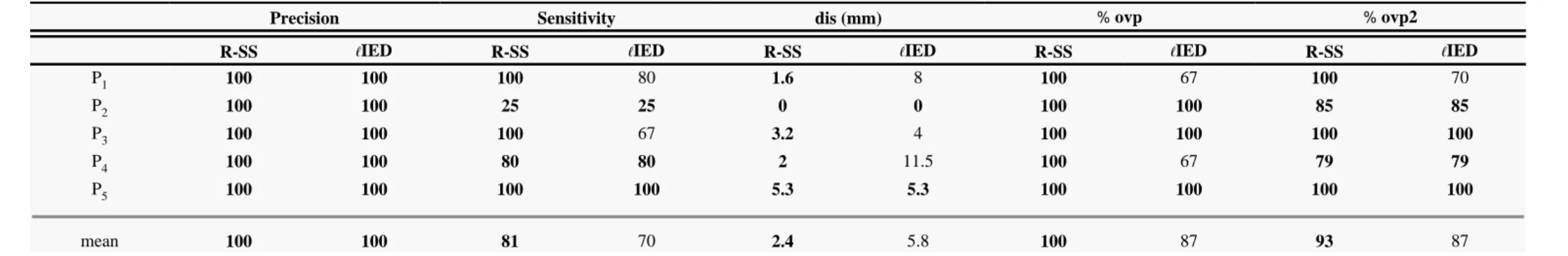
Our method provides a greater congruency with vSOZ in comparison with IED regions. This result is shown quantitatively in Tableℓ
II. In this table, the IED regions estimated by our method and IED regions are compared with vSOZ by assuming that vSOZs are theℓ
ground truth. For this purpose, the following measures are used.
/( ) (in ), where and indicate true positive and false positive in terms of brain regions, respectively.
Precision=TP TP+FP % TP FP TP
is the number of common brain regions between vSOZ and our estimated IED regions, while FP is the number of uncommon regions which were falsely detected by our method.
/( ) (in ), where indicates the false negative in terms of brain regions. is the number of regions missed
Sensitivity=TP TP+FN % FN FN
by our method.
: the average of minimum distances (mm) between IED and vSOZ electrode leads. The smaller this value, on average, the closer the
dis
set of IED regions to vSOZ.
: the average percentage of the number of IED electrode leads that are in the neighborhood ( 1.5 cm) of at least one of the vSOZ
ovp <
electrode leads. ovp 100 shows that we obtained at least one IED electrode lead in proximity of each of vSOZ electrode leads.= %
Conversely, ovp 0 shows that we could not obtain any IED electrode lead in proximity of any of vSOZ electrode leads.= %
2: the average percentage of the number of vSOZ electrode leads that are in the neighborhood ( 1.5 cm) of at least one of the IED
ovp <
Evaluation of the Proposed Method in Terms of Robustness
The robustness of the method is evaluated according to the influence of the number of IED time intervals and errors in identification of IED time intervals.
Number of IED Time Intervals
The proposed GEVD-based method is fast due to its exact analytic solution, but the correct estimation of correlation matrices is important for the reliability of the results. Large enough number of data samples in each IED or non-IED time interval is needed for a proper estimation of correlations. The length of each IED time interval depends on the length of single or bursts of IEDs. Here, the mean of minimum and maximum length of IED time intervals over patients is equal to 236 and 3.3 10 samples, respectively, which provides× 3 statistically reliable estimation of correlation matrices.
The length of the required recorded data for processing is dependent on the number of IED and non-IED time intervals that exists in this length of data. It means that if in a given set of data there does not exist enough number of IED and non-IED time intervals, we need longer set of data to obtain the sufficient number of IED and non-IED time intervals. In our recordings, the mean of the length of selected data is about 1 h. To reduce the number of IED or non-IED time intervals (not the length of each time interval), and eventually reduce the required time length of data for recording, we test the reliability of the method in terms of the number of IED time intervals. For this purpose, we use the jackknife method as follows. First, a percentage ( ) of available IED and non-IED time intervals is selected randomly.L
Next, the IED electrode leads related to these time intervals (IED ) are estimated. Finally, the related false positive and false negative (# FP
and FN) measure values are calculated in terms of electrode leads (for more details, see the Appendix). By repeating this procedure 100 times, the mean and standard deviation of FP and FN are calculated (see the left column in Fig. 3). We assume that the set of IED electrode leads using 100 of available IED and non-IED time intervals is the ground truth. is set to 30 and 70 . Therefore, weL= % L % %
consider that the results of the method are reliable for L < 100 , if there is no significant change between the results related to % L < 100%
and 100 .L= %
Results of Fig. 3 (left column) can show the reliability of the method for small number of IED time intervals (about 50) for most of the patients (P1 –P ). For P , the standard deviation is higher in comparison with other patients, which reveals its sensitivity for small number4 5 of IEDs.
Errors in Identification of IED Time Intervals
To test the effect of possible errors in identification of IED time intervals (due to expert variability, or in the future the error in automatic labeling), we exchange the labels of a randomly selected percentage ( ) of available IED and non-IED time intervals, andE
estimate the related IED electrode leads (IED ). The same jackknife-based method explained previously is applied. Here, we assume the# ground truth is the set of IED electrode leads estimated by using original IED and non-IED labels, i.e., 0 . is set equal to 10 , 20 ,E= % E % %
30 , 40 , and 50 . Therefore, if there is no decrease of performance for each of the former error percentages in comparison with 0 ,% % % E= %
we can conclude that the method can tolerate this percentage of error in IED labeling. Fig. 3 (right column) shows the mean and standard deviation of FP and FN for all the patients. The result shows the importance of the discriminative information between the two IED and non-IED states and how it is crucial for obtaining the proper results. According to Fig. 3 (right column), one can conclude that 10 error%
in labeling again provides correct results for most of patients: only the results of P are very sensitive to the error of labeling.1
Discussion
Simulation Evaluation
The simulated data are a simplified example of real data, where we assume the presence of two epileptic sources in the volume around the electrodes, supposed to be inserted in a clinically suspected brain area. We are not looking for a unique solution in our method; instead, we are interested in extracting a set of solutions, in which the number of solutions is practically unknown. Using the Pareto optimality concept and eventually classification of the search space into different nondominated layers, we aim to estimate the set of electrode leads that are the closest to at least one of the epileptic sources. As can be seen in Fig. 2, the first nondominated layer includes mostly the electrodes that are the closest to epileptic sources in the three simulations with different orientations of epileptic sources. These leads are not necessarily close to a single source; instead, these are the leads which receive a greater contribution from at least one of the epileptic sources, and eventually. they have higher membership probability to IED class. Since dmax ≤ ε || || (see Section II-D), and thus the secondp
layer is close enough to the first layer, we enlarge the set of results by considering the former one. Therefore, we obtain extra electrode leads in the neighborhood, such as A , C , and B . By considering the second layer results, we can see if there is any solution in the1 8 0 neighborhood (even with less membership probability in comparison with first layer) which might be useful for the epileptologists. In this paper, we do not identify the location and orientation of the dipole sources. However, these extra information is very helpful for future works for localizing the dipole sources in respect to the location of neighborhood electrode leads.
For the three simulations of different orientations, most of the estimated IED leads are common. Some of the differences between the set of results are electrode leads A and A . A is identified for the three orientations except D . This is the specific condition in which the1 2 1 1 angle between the source dipole e and position vector of A is perpendicular. A is less specific since there are other nonepileptic sources1 1 2 close to this lead.
The method performs well over a large range of SIR values (SIR ∈ [−2, 20 dB), as the same set of electrode leads is always+ ]
identified. Although decreasing SIR decreases the number of electrodes in the first layer, all the significant electrodes (A and C ) are0 9 identified for even the lowest SIR value.
Advantages of Using GEVD
In most usual BSS methods, identification of sources related to the desired state is done in two steps. The sources are first estimated, and then, the sources of interest are selected usually by correlation with the reference. On the contrary, in GEVD, the two tasks are done in a unique step, since the estimated sources are ranked according to their similarity to the reference model. Therefore, we only need to identify the number of related sources. In addition, GEVD does not require the assumption of either independence or non-Gaussianity as it is done in independent component analysis (ICA) methods. However, it would obviously lead to decorrelated sources. Since in our application, the sources are not necessarily independent, GEVD is more flexible. Finally, solving GEVD is very fast and only based on second-order statistics contrary to ICA which requires higher order statistics.
Comparison Between dDCG-Based and R-SS Identification Methods
The dDCG-based identification method considers causal relationships, discriminating between regions originating the IED signals (sources or leading IED regions) and the regions receiving the propagated IED signals (sink regions). This property does not hold in the R-SS method. However, the dDCG method is time consuming due to the permutation calculations in the graph construction 7 . On the[ ]
contrary, the R-SS method is simple and fast as its solution is based on an analytical mathematic problem, i.e., GEVD. This property is valuable for an online process of iEEG recordings. The processing time of the R-SS method for about 40 min of recording which provides 195 IED and non-IED time intervals and for 111 channels is about 4 min, while it is about 100 times longer for dDCG (using a shared 3-GHz, 4-core Xeon 64 bits processor). Another advantage of R-SS over dDCG is that R-SS can provide reliable results for less number of IED and non-IED time intervals (about 50 time intervals). For construction of dDCG that is based on multiple test using permutations, to obtain statistically reliable results, about 150 time intervals are needed for false alarm rate equal to 0.05, 100 connections, and 10 000 permutations. R-SS just requires enough number of samples in each time interval for a statistically reliable estimation of correlation matrices.
One current limitation of both dDCG and R-SS methods is using the manual labeling of IED and non-IED time intervals. This information is crucial for estimating the IED regions for both methods correctly. However, R-SS can tolerate 10 of errors in the labeling.%
Conclusion
In this paper, we propose a new R-SS method using GEVD for identification of brain regions involved in a reference brain state (interictal events) from iEEG recordings. Using GEVD, we estimate the spatial filter that maximizes the power of IED over non-IED state and provides temporal sources ranked according to their similarity to IED state. Using these temporal sources and their corresponding spatial patterns, each electrode lead is represented as an -dimensional feature vector. The number of sources of IED class is estimatedi* i*
automatically based on Bayes probability error. By applying the Pareto optimization method on the feature vector values of all the’
electrode leads, we obtain the electrode leads with significantly large IED activity that build the estimated IED regions.
The method is applied on the iEEG recordings of five patients suffering from epilepsy. All patients are seizure-free after resective surgery. The IED regions estimated by our method are congruent with SOZ visually inspected by an epileptologist and another automatic method 7 for these five patients. The method requires two sets of intervals, i.e., IED (or reference) and non-IED. The correct labeling of[ ]
these intervals is crucial for obtaining the congruent results, but 10 of errors in labeling does not make a significant change in the results.%
The proposed method is also reliable for small number (about 50) of IED and non-IED time intervals. However, each time interval should include enough number of samples for statistically reliable estimation of correlations.
The efficiency of the method is also evaluated qualitatively using simple simulated data. A complete study on more number of simulated data for the analysis of the effect of different parameters and their related quantitative evaluations is our first perspective. One limitation of the method is the manual labeling of IED and non-IED time intervals: automatic detection is thus a second perspective. As a third perspective, the proposed method must be applied on a larger number of simulations and patients for a more complete validation. A fourth perspective could be using the R-SS method as a preprocessing step for dDCG construction for decreasing its computation time. For this purpose, we can apply R-SS to find IED-related electrode leads and then calculate dDCG for these electrode leads to estimate the robust differential network between them. Therefore, for a limited number of electrode leads, the computations for dDCG would be much
faster. Finally, localization of the epileptic sources by solving the inverse problem can also be considered as future works to obtain better localization for epileptic sources.
Acknowledgements:
The authors gratefully acknowledge P. Kahane, L. Vercueil, O. David, L. Minotti (from Grenoble Institute of Neuroscience, U836 INSERM, and/or Neurology Department, CHUG, Grenoble, France), and F. Wendling (from Inserm 1099, Signal and Image Processing Laboratory, University of Rennes 1) for providing the data, interpretations, and their helpful assistance in this study.
Appendix False positive and false negative in terms of electrode leads
and are calculated between members of and is the set of estimated IED electrode leads of each recalculated trial and
FP FN IED# GT. IED#
members of GT are assumed as the ground truth. We calculate the Euclidean distance, , between the th member of d i IED and th member of # j
, where 1, , , 1, , . We threshold giving 1 if , otherwise zero. LFP stands for local field potential. According to 23
GT i= … N′ j= … N d b= dLFP [ ]
, the LFP recorded from each electrode lead can be related to a neural population within 0.5 3 mm of the electrode tip. In 24 , an LFP– [ ]
coherence about 0.15 0.35 (0 coherence 1) for approximately 3 4 mm primary visual cortical distance was reported for frequency range of– < < –
2 60 Hz. In our recordings, the interdistance between two adjacent electrode leads is 3.5 mm, so for the thresholds less than this distance,–
there is no neighbor electrode lead at least on a single electrode. As such thLFP equal to 4 mm is chosen. FP and FN are calculated as
Footnotes:
1 Note that in the two inequalities, one of them is a strict inequality.
2 Here, signal is related to epileptic sources, and interference to nonepileptic (background) sources. The SIR is then calculated for the significant electrodes, A0 and C9, by computing the power ratio (in decibels) of the signals related to the epileptic sources ( and ) overe1 e2
all the signals related to the nonepileptic sources.
References:
1 .Rosenow F , L ders ü H . Presurgical evaluation of epilepsy . Brain . 124 : (9 ) 1683 - 1700 2001 ;
2 .Alarcon G , Seoane JJG , Binnie CD , Miguel MCM , Juler J , Polkey CE , Elwes RD , Blasco JMO . Origin and propagation of interictal discharges in the acute electrocorticogram. implications for pathophysiology and surgical treatment of temporal lobe epilepsy . Brain . 120 : (Pt 12 ) 2259 - 2282 Dec 1997 ;
3 .Alarcon G . Electrophysiological aspects of interictal and ictal activity in human partial epilepsy . Seizure . 5 : (1 ) 7 - 33 Mar 1996 ;
4 .Hufnagel A , Dumpelmann M , Zentner J , Schijns O , Elger CE . Clinical relevance of quantified intracranial interictal spike activity in presurgical evaluation of epilepsy . Epilepsia . 41 : (4 ) 467 - 478 Apr 2000 ;
5 .Bourien J , Bartolomei F , Bellanger J , Gavaret M , Chauvel P , Wendling F . A method to identify reproducible subsets of co-activated structures during interictal spikes. application to intracerebral EEG in temporal lobe epilepsy . Clin Neurophysiol . 116 : (2 ) 443 - 455 2005 ;
6 .Marsh ED , Peltzer B , Brown MW III , Wusthoff C , Storm PB Jr , Litt B , Porter BE . Interictal EEG spikes identify the region of electrographic seizure onset in some, but not all, pediatric epilepsy patients . Epilepsia . 51 : (4 ) 592 - 601 2010 ;
7 .Amini L , Jutten C , Achard S , David O , Soltanian-Zadeh H , Hossein-Zadeh GA , Kahane P , Minotti L , Vercueil L . Directed differential connectivity graph of interictal epileptiform discharges . IEEE Trans Biomed Eng . 58 : (4 ) 884 - 893 Apr 2011 ;
8 .Sameni R , Jutten C , Shamsollahi M . Multichannel electrocardiogram decomposition using periodic component analysis . IEEE Trans Biomed Eng . 55 : (8 ) 1935 - 1940 Aug 2008 ;
9 .De Lathauwer L , De Moor B , Vandewalle J . SVD-based methodologies for fetal electrocardiogram extraction . Proc IEEE Int Conf Acoust Speech Signal Process . 2000 ; 6 : 3771 - 3774
10 .Cosandier-Rim l é éD , Badier J , Chauvel P , Wendling F . A physiologically plausible spatio-temporal model for EEG signals recorded with intracerebral electrodes in human partial epilepsy . IEEE Trans Biomed Eng . 54 : (3 ) 380 - 388 Mar 2007 ;
11 .Borga M . Learning multidimensional signal processing . PhD dissertation . Linkping Univ ; Linkping, Sweden 1998 ;
12 .Sameni R , Jutten C , Shamsollahi M . A deflation procedure for subspace decomposition . IEEE Trans Signal Process . 58 : (4 ) 2363 - 2374 Apr 2010 ; 13 .Pham DT , Cardoso JF . Blind separation of instantaneous mixtures of nonstationary sources . IEEE Trans Signal Process . 49 : (9 ) 1837 - 1848 Sep 2001 ;
14 .Samadi S , Amini L , Soltanian-Zadeh H , Jutten C . Identification of brain regions involved in epilepsy using common spatial pattern . Proc. IEEE Workshop Stat. Signal Process. Nice, France Jun. 2011 825 - 828
15 .Fukunaga K , Koontz W . Application of the Karhunen-Loeve expansion to feature selection and ordering . IEEE Trans Comput . C-19 : (4 ) 311 - 318 Apr 1970 ; 16 .Gouy-Pailler C , Congedo M , Brunner C , Jutten C , Pfurtscheller G . Multi-class independent common spatial patterns: Exploiting energy variations of brain sources . Proc. 4th Int. Brain-Comput. Interf. Workshop Train. Course Graz, Austria Sep. 2008 20 - 25
17 .Bragin A , Wilson CL , Engel J . Chronic epileptogenesis requires development of a network of pathologically interconnected neuron clusters: A hypothesis . Epilepsia . 41 : S144 - S152 2000 ;
18 .Deb K . Multi-objective evolutionary algorithms: Introducing bias among pareto-optimal solutions . Kanpur Genetic Algorithms Lab ; Kanpur, India Tech Rep . 99002 : 1999 ;
19 .Branke J , Deb K , Miettinen K , Slowinski R . Multiobjective Optimization, Interactive and Evolutionary Approaches . New York, NY, USA Springer ; 2008 ; 20 .Chang N , Gulrajani R , Gotman J . Dipole localization using simulated intracerebral EEG . Clin Neurophysiol . 116 : (11 ) 2707 - 2716 2005 ;
21 .Wendling F , Bellanger JJ , Bartolomei F , Chauvel P . Relevance of nonlinear lumped-parameter models in the analysis of depth-EEG epileptic signals . Biol Cybern . 83 : (4 ) 367 - 378 Oct 2000 ;
22 .Amini L . Development of differential connectivity graph for characterization of brain regions involved in epilepsy . PhD dissertation, cotutelle between Control and Intelligent Processing Center of Excellence, School of ECE, Faculty of Engineering, Univ Tehran, Tehran, Iran, and Image, Speech, Signal, and Automatic laboratory of Grenoble, Univ Grenoble, Grenoble Cedex, France . 2010 ;
23 .Juergens E , Guettler A , Eckhorn R . 1999 ; Visual stimulation elicits locked and induced gamma oscillations in monkey intracortical- and eeg-potentials, but not in human EEG . Exper Brain Res Online [ ]. 129 : 247 - 259 Available: http://dx.doi.org/10.1007/s002210050895
Fig. 1
R-SS method. and , 1, m= …, denote the correlation matrices of different IED and non-IED time intervals, respectively. TheLℓ
averages of these matrices denoted as R 1 and R 2 are the inputs of GEVD. Using GEVD, the discriminative temporal sources, , 1, s i= …, ,N are estimated. These sources are ranked according to their similarity to the IED class.
Fig. 2
Schematic diagram of simulated data. Three electrodes (A, B, and C), six nonepileptic and two epileptic (e and e ) sources in three different1 2 orientations (D , D , and D ) are demonstrated. The squares indicate the electrode leads. Each electrode consists of ten equally spaced0 1 2 recording contacts (3.5-mm intercontact spacing). The thick and thin frames demonstrate the first and second layer nodes of Pareto, respectively.
Fig. 3
Mean and standard deviation of FP (solid) and FN (dashed) for different percent of IED time intervals (left), and different error percentages of IED labeling (right) for five patients. From top to bottom, P to P .1 5
TABLE I
Comparison Between the Visually Inspected SOZ (vSOZ) By the Epileptologist, the Leading IED Regions ( IED Regions) Estimated Based on dDCG and the IED Regions Estimated By the R-SSℓ
Method
P1 antHC postHC pHcG amyg mTP
vSOZ × × × × ×
ℓIED × × × ×
R-SS × × × × ×
P2 antHC postHC pHcG amyg
vSOZ × × × × ℓIED × R-SS × P3 antHC postHC pHcG vSOZ × × × ℓIED × × R-SS × × ×
P4 antHC postHC amyg mTP entC
vSOZ × × × × × ℓIED × × × × R-SS × × × P5 midInsG vSOZ × ℓIED × R-SS ×
TABLE II
Quantitative Comparison Between IED Regions Based on dDCG and IED Regions Based on R-SSℓ
Precision Sensitivity dis (mm) % ovp % ovp2
R-SS ℓIED R-SS ℓIED R-SS ℓIED R-SS ℓIED R-SS ℓIED
P1 100 100 100 80 1.6 8 100 67 100 70 P2 100 100 25 25 0 0 100 100 85 85 P3 100 100 100 67 3.2 4 100 100 100 100 P4 100 100 80 80 2 11.5 100 67 79 79 P5 100 100 100 100 5.3 5.3 100 100 100 100 mean 100 100 81 70 2.4 5.8 100 87 93 87