4D-Var Assimilation of MIPAS chemical observations: ozone and nitrogen dioxide analyses

HAL Id: hal-00304129

https://hal.archives-ouvertes.fr/hal-00304129

HAL is a multi-disciplinary open access

archive for the deposit and dissemination of sci-entific research documents, whether they are pub-lished or not. The documents may come from teaching and research institutions in France or abroad, or from public or private research centers.

L’archive ouverte pluridisciplinaire HAL, est destinée au dépôt et à la diffusion de documents scientifiques de niveau recherche, publiés ou non, émanant des établissements d’enseignement et de recherche français ou étrangers, des laboratoires publics ou privés.

4D-Var Assimilation of MIPAS chemical observations:

ozone and nitrogen dioxide analyses

Q. Errera, F. Daerden, S. Chabrillat, J. C. Lambert, W. A. Lahoz, S.

Viscardy, S. Bonjean, D. Fonteyn

To cite this version:

Q. Errera, F. Daerden, S. Chabrillat, J. C. Lambert, W. A. Lahoz, et al.. 4D-Var Assimilation of MIPAS chemical observations: ozone and nitrogen dioxide analyses. Atmospheric Chemistry and Physics Discussions, European Geosciences Union, 2008, 8 (2), pp.8009-8057. �hal-00304129�

ACPD

Full Screen / Esc

Printer-friendly Version

Interactive Discussion Atmos. Chem. Phys. Discuss., 8, 8009–8057, 2008

www.atmos-chem-phys-discuss.net/8/8009/2008/ © Author(s) 2008. This work is distributed under the Creative Commons Attribution 3.0 License.

Atmospheric Chemistry and Physics Discussions

4D-Var Assimilation of MIPAS chemical

observations: ozone and nitrogen dioxide

analyses

Q. Errera1, F. Daerden1, S. Chabrillat1, J. C. Lambert1, W. A. Lahoz2, S. Viscardy1, S. Bonjean1,*, and D. Fonteyn1,**

1

Insitut d’A ´eronomie Spatiale de Begique, BIRA–IASB, Belgium

2

Norsk Institutt for Luftforskning, NILU, Norway

*

now at: Sputnik Web, Belgium

**

now at: Belgian Federal Science Office, Belgium

Received: 11 January 2008 – Accepted: 26 March 2008 – Published: 22 April 2008 Correspondence to: Q. Errera (quentin.errera@aeronomie.be)

ACPD

Full Screen / Esc

Printer-friendly Version

Interactive Discussion

Abstract

This paper discusses the global analyses of stratospheric ozone (O3) and nitrogen dioxide (NO2) obtained by the Belgian Assimilation System for Chemical Observations from Envisat (BASCOE). Based on a chemistry transport model (CTM) and the 4-dimensional variational (4D-Var) method, BASCOE has assimilated chemical

obser-5

vations of O3, NO2, HNO3, N2O, CH4 and H2O, made between July 2002 and March 2004 by the Michelson Interferometer for Passive Atmospheric Sounding (MIPAS) on-board the European Space Agency (ESA) Environment Satellite (ENVISAT). This cor-responds to the entire period during which MIPAS was operating at its nominal resolu-tion.

10

Our analyses are evaluated against assimilated MIPAS data and independent HALOE (HALogen Occultation Experiment) and POAM-III (Polar Ozone and Aerosol Measurement) satellite data. A good agreement is generally found between the analy-ses and these datasets, in both caanaly-ses within the estimated error bars of the observa-tions. The benefit of data assimilation is also evaluated using a BASCOE free model

15

run. For O3, the gain from the assimilation is significant during ozone hole conditions, and in the lower stratosphere. Elsewhere, the free model run is within the MIPAS un-certainties and the assimilation does not provide significant improvement. For NO2, the gain from the assimilation is realized through most of the stratosphere. Using the BASCOE analyses, we estimate the differences between MIPAS data and independent

20

data from HALOE and POAM-III, and find results close to those obtained by classical validation methods involving only direct measurement-to-measurement comparisons. Our results extend and reinforce previous MIPAS data validation efforts by taking ac-count of a much larger variety of atmospheric states and measurement conditions.

This study discusses possible further developments of the BASCOE data

assimila-25

tion system; these concern the horizontal resolution, a better filtering of NO₂ observa-tions, and the photolysis calculation near the lid of the model. The ozone analyses are publicly available via the PROMOTE project (http://www.gse-promote.org).

ACPD

Full Screen / Esc

Printer-friendly Version

Interactive Discussion

1 Introduction

Data assimilation is a set of well-known methods that are used to map observations onto a regular grid using the laws of the atmosphere (or other system of interest) em-bodied in a numerical model. In principle, the resulting “analyses” provide the best estimate of the state of the atmosphere. In numerical weather prediction (NWP), these

5

analyses are used to provide weather forecasts. On the other hand, assimilation sys-tems based on chemical transport models (CTMs) or photochemical box model have broader goals (Lahoz et al.,2007), one of them being the validation of satellite data (Marchand et al.,2004;Vigouroux et al.,2007).

The Michelson Interferometer for Passive Atmospheric Sounding (MIPAS)

in-10

strument on board of ESA’s ENVISAT satellite measures the Earth limb emission infrared spectra, from which ESA operational level-1-to-2 processors retrieve the vertical distribution of several key stratospheric species: ozone (O₃), nitric acid (HNO3), nitrogen dioxide (NO2), nitrous oxide (N2O), water vapour (H2O), and methane (CH4). Several operational centres and research institutes

as-15

similated MIPAS O₃ data successfully using systems based on various model types (CTMs, or general circulation models, GCMs) and various assimilation methods (sequential and variational, e.g.,Dethof,2003;Wargan et al.,2005;Geer et al.,2006). In particular,Baier et al.(2005) assimilated all the six operational MIPAS constituents. Nevertheless, the above-mentioned studies addressed only a few months of MIPAS

20

data, making it difficult to obtain robust statistics valid for a complete annual cycle of atmospheric states and measurement conditions. This study presents, for the first time, an assimilation of the entire MIPAS level-2 data record available at nominal resolution (July 2002 to March 2004, i.e. 21 months). The assimilation has been performed by the BASCOE (Belgian Assimilation System of Chemical Observations

25

from ENVISAT) 4D-Var data assimilation system. BASCOE is based on a 3D–CTM driven by meteorological analyses of winds and temperature provided by the European Centre for Medium-range Weather Forecasts (ECMWF). Near real time assimilation

ACPD

Full Screen / Esc

Printer-friendly Version

Interactive Discussion of MIPAS level 2 data and short-term chemical forecasts have also been made with

an earlier version of BASCOE within the framework of ENVISAT cal/val activities (Fonteyn et al.,2002,2004, see alsohttp://bascoe.oma.be).

The present paper presents and discusses the assimilation of MIPAS level-2 data re-trieved with ESA’s off-line Instrument Processing Facility (IPF) versions 4.61 and 4.62.

5

We focus on analyses of O3 and NO2. Monitoring of independent observations from HALOE (HALogen Occultation Experiment) and POAM-III (Polar Ozone and Aerosol Measurement) is also achieved during the assimilation procedure; this has not been done in previous MIPAS assimilation studies. The monitoring procedure allows com-parison of the BASCOE analyses against HALOE and POAM-III data in an optimal

10

way. Based on our analyses, we estimate the bias and standard deviation between MIPAS and independent data and our results are compared with those obtained by classical validation methods limited to direct measurement-to-measurement compar-isons. HALOE, POAM-III and MIPAS data have also been monitored with a six-month free model run, initialized with analysed data. Comparison between the analyses and

15

the free model run allows us to discuss the added value provided by data assimilation. What is new in this paper are: (1) the extended assimilation period (especially for NO₂) which allows us to derive robust statistics valid for the widest range of atmospheric states and measurement conditions; (2) the monitoring procedure, which allows us to evaluate the datasets in an optimal manner; and (3) the use of BASCOE analyses

20

to derive differences between MIPAS and independent data from HALOE and POAM-III, even in absence of direct collocation of the air masses measured by the different satellites.

The paper is organized as follows. Sections 2, 3 and 4 describe, respectively, the BASCOE system, the data used in this study and the set-up of the assimilation

experi-25

ments. Sections 5 and 6 discuss, respectively, the O₃and NO₂analyses. Conclusions and possible further developments are given in Sect. 7.

ACPD

Full Screen / Esc

Printer-friendly Version

Interactive Discussion

2 System description

The Belgian Assimilation System of Chemical Observations from ENVISAT (BASCOE,

http://bascoe.oma.be) is a 4-dimensional variational (4D-Var) system descended from that described inErrera and Fonteyn(2001). Model studies of the 2003 Antarctic winter using the BASCOE CTM coupled with a Polar Stratospheric Cloud (PSC)

microphysi-5

cal scheme can be found inDaerden et al.(2007). Fonteyn et al.(2002,2004) used a version of BASCOE that includes the microphysical scheme for near real time assimi-lation of MIPAS. A version of BASCOE close to the one presented here has also been used in the framework of the validation of MIPAS HNO₃ and N₂O (Vigouroux et al.,

2007).

10

In the BASCOE version presented here, the microphysical scheme has been re-placed by a parameterization to reduce the computing time. Nevertheless, this latest version has also the capability to run in near real time.

2.1 The 3D–CTM

All chemical species are advected using the Flux Form Semi-Lagrangian scheme (Lin 15

and Rood,1996) with a time step of 30 min; The CTM is driven by ECMWF operational analyses of winds and temperatures, and uses a subset of 37 of the 60 ECMWF model levels, from the surface to 0.1 hPa, on a 5◦longitude by 3.75◦ latitude grid. The model grid type is Arakawa C (Kalnay,2003).

The model includes 57 chemical species with a full description of stratospheric

chem-20

istry. The species interact through 143 gas-phase reactions, 48 photolysis reactions and 9 heterogeneous reactions. The chemical system of differential equations is built using the Kinetic PreProcessor (Damian et al.,2002) and is integrated with a third-order Rosenbrock solver (Hairer and Wanner,1996). The reaction rates and cross-sections are taken from the JPL compilation Evaluation 14 (Sander et al.,2003).

25

The Surface Area Density (SAD) of sulfate aerosols is prescribed as a function of pressure and latitude, using the climatological distribution described byDaerden et al.

ACPD

Full Screen / Esc

Printer-friendly Version

Interactive Discussion (2007). WhileDaerden et al.(2007) couple a PSC microphysical scheme to the CTM,

here we use a parameterization that sets the surface area density of PSCs and calcu-lates the loss of HNO3and H2O by PSC sedimentation as a function of temperature. Ice PSCs are presumed to exist in the winter/spring Polar Regions at any grid point where the temperature is colder than 186 K, and Nitric Acid Tri-hydrate (NAT) PSCs

5

at any grid point where the temperature is colder than 194 K. The surface area den-sity is set to 10−6cm−2/cm−3 for ice PSCs and 10−7cm−2/cm−3 for NAT PSCs. The sedimentation of PSC particles causes denitrification and dehydration. This process is also approximated in a very simple way, by an exponential decay of HNO3 with a characteristic time–scale of 100 days for gridpoints where NAT particles are supposed

10

to exist, and an exponential decay of HNO₃and H₂O with a characteristic time-scale of 9 days for gridpoints where ice particles are supposed to exist (Solomon and Brasseur,

1997).

All species simply have null flux as upper and lower boundary conditions. While the model extends down to the surface, it does not include any tropospheric process and

15

is not expected to produce a realistic chemical composition below the tropopause.

2.2 The 4D-Var system

Data assimilation is done using 4D-Var (Talagrand and Courtier, 1987). This method optimizes the model initial conditions to reproduce a set of observations over a time window. This is done by minimizing the following objective function,J(x) (also denoted

20

cost function) (Talagrand and Courtier,1987):

J(x) = 1 2[x(t0)− x b_(t 0)]TB−1₀ [x(t0)− xb(t0)] + (1) 1 2 N X i =0 (yo(ti)− H(x(ti)])TR−1_i (yo(ti)− H(x(ti)])

ACPD

Full Screen / Esc

Printer-friendly Version

Interactive Discussion given the model evolution equation

x(ti) = Mi −1[x(ti − 1)] (2)

where x(t_i) represents the model state vector at time t_i, xb(t₀) is the first guess and

B0 is the background covariance matrix of x

b

(t0). Vectors y

o

(t_i) and matrix R_i are, respectively, the observation state vector and the error covariance matrix associated

5

with the observations at timeti. The observation operatorH maps the model state into

the observation space andM is the model operator that calculates the time evolution

of the model state. Minimization of Eq. (1) requires the knowledge of the gradient ofJ.

This is done using the adjoint of the forward (or direct) model. The minimization of the objective function uses the quasi-Newton algorithm M1QN3 (Gilbert and Lemarechal,

10

1989) and the system is preconditioned (Bouttier and Courtier,2002).

Three processes in the BASCOE model affect chemical concentrations: advection, chemistry and the PSC parameterization. The adjoint code of these processes is re-quired for implementation of 4D-Var. Although the number of species and reactions, and the advection scheme have changed sinceErrera and Fonteyn(2001), their adjoint

15

has been built following the same procedure. The adjoint of the PSC parameterization has been built by hand. Note that several approaches can be used to build chemistry adjoints (see Sandu et al., 2003, for a review). In one approach, the adjoint of the chemistry is the adjoint of the chemical system of equations and the backward inte-gration in time is done with the same integrator as for the forward case, as is done in

20

Errera and Fonteyn(2001). Sandu et al.(2003) discuss what they term the continuous and discrete approaches to the calculation of chemistry adjoints. In this context, the approach ofErrera and Fonteyn(2001) falls in the continuous category. If one wishes to avoid this approximation, which means using the discrete approach, the adjoint of the integrator for the backward case should also be built.

25

Because the set-up ofErrera and Fonteyn(2001) gave good results, it was used in the formulation of the BASCOE adjoint. However, there are four time periods where the minimization is not attained, i.e., the system is not able to reduceJ during the iteration

ACPD

Full Screen / Esc

Printer-friendly Version

Interactive Discussion process. These periods are: (1) 6 days in September 2002, during the Antarctic vortex

split; (2) 6 days during mid February 2002; (3) 15 days during March 2003; and (4) 17 days between mid September and the beginning of October 2003.

The reasons for this failure are still under investigation. However, there are clues that point to possible causes. For example, the problem occurs with data located above

5

3 hPa and in the Polar Regions. We do not think that the source of this problem is due to the observations because: (1) data corresponding to days without minimization are not so different than data for days where the minimization is achieved; and (2) a data filter is already implemented to reject outliers (see Sect.4). It is more likely that the fast dynamical changes that can occur in the high Polar Stratosphere are not compatible

10

with the approximations used to calculate the adjoint of the chemistry. As a result, small errors arising from these approximations are amplified by the adjoint of the transport.

In order to provide the most complete dataset of analyses and avoid problematic cases, we choose to filter out all observations for levels above 3 hPa and for latitudes poleward of| ± 50◦| for these days.

15

3 The observations

Three satellite datasets are used in this study: MIPAS data are assimilated by the BASCOE system to constrain its CTM outputs, while HALOE and POAM-III data are monitored by the system and used for a posteriori evaluation of the BASCOE analyses. In the monitoring procedure, BASCOE searches for any observations from HALOE

20

and POAM-III at each model time step. If any measured profile is found within a time window of 30 min around the model time step, geographically surrounding BASCOE profiles are interpolated spatially to the tangent point geolocation of the HALOE or POAM-III measurements, and saved into a file. Using this method, there is no tempo-ral interpolation, and the maximum time mismatch between measurement and model

25

values is 15 min. This is an important detail, especially for NO₂evaluation, given the diurnal cycle of this species and its rapid variation at scales of minutes during twilight.

ACPD

Full Screen / Esc

Printer-friendly Version

Interactive Discussion Note that, unlike in NWP centers, the monitoring procedure is not commonly used by

the assimilation system of research institutes. Note that BASCOE analyses are also saved in the MIPAS observation space.

3.1 MIPAS

The ENVISAT MIPAS instrument measures nighttime and daytime Earth limb

emis-5

sion high-resolution spectra with a Michelson interferometer (Fischer et al.,2000). The vertical distribution of numerous atmospheric trace gas can be retrieved from MIPAS spectra using Fourier Transform spectroscopy. Here, the six chemical species retrieved operationally by ESA’s off-line processor are assimilated: O3, HNO₃, H₂O, NO₂, N₂O and CH4. All species are assimilated together without any distinction of day or night

10

data. Usually there are around 1000 MIPAS profiles per day. Twenty-one months of data have been assimilated (18 July 2002–26 March 2004). We combine off-line ver-sions 4.61 and 4.62 to increase the period of MIPAS observations: for example, after 7 December 2003, only v4.62 data are available. However, each daily dataset comes from a single version. Both ozone (v4.61 and v4.62,Cortesi et al.,2007) and nitrogen

15

dioxide (v4.61,Wetzel et al.,2007) have been validated for scientific applications. Be-tween 1 to 50 hPa, the ozone bias with respect to correlative data is lower than 10%; it increases to 25% at 100 hPa. At levels above 1 hPa, the number of correlative data are too small to derive quantitative conclusions (Cortesi et al.,2007). In the lower and mid-dle stratosphere (below 45 km), the accuracy and precision of MIPAS NO2is 10–20%

20

and 5–15%, respectively (Wetzel et al.,2007).

3.2 HALOE

Operating aboard NASA’s Upper Atmosphere Research Satellite (UARS) from 1991 through 2005, HALOE (Russell III et al.,1993) used solar occultation to measure at-mospheric constituent profiles of O₃, NO, NO₂, HCl, CH₄, HF and aerosol extinction.

25

ACPD

Full Screen / Esc

Printer-friendly Version

Interactive Discussion The 56◦inclination of the UARS orbit generated a small daily precession of the latitude

of the sunrises and sunsets, yielding global coverage from 50◦S–80◦N to 50◦N–80◦S in about one month. Version 19 of HALOE, the latest version available publicly, is used here to validate the BASCOE analyses. Intercomparison of ozone with correlative data (acquired by ozonesonde, lidar, balloon-borne remote sensing, rocketsondes and other

5

satellites) shows good agreement, usually within the estimated measurement errors, between 0.03 to 100 hPa. HALOE ozone errors are 11% at 0.1 hPa, 5% between 1 and 30 hPa, and gradually increase to 30% at 100 hPa (Br ¨uhl et al., 1996, for version 17; see Sect. 3.3 for version 19 updates). For levels below 120 hPa, HALOE profiles can be seriously affected by the presence of aerosols and cirrus clouds (Bhatt et al.,1999).

10

The HALOE NO and NO2 measurements have been validated using satellite, balloon and ground based measurements (Gordley et al.,1996, for version 17). In the middle stratosphere, the NO₂measurements show mean differences with independent data of about 10 to 15%. NO differences in the middle stratosphere are similar, but sometimes show a negative bias (as much as 35%) between 30 and 60 km with some correlative

15

measurements. In this study, analyses of NO_x (NO+NO2) are compared with HALOE NOx. This is done to minimize the error at the terminator due to the maximum time shift of 15 min between BASCOE analyses and observations (see above).

3.3 POAM-III

Owing to the polar orbit of the SPOT-4 platform (98.6◦ inclination), POAM-III, which is

20

also a solar occultation instrument, measures the vertical distribution of the chemical stratospheric constituents O3, NO2, H2O and aerosol extinction in the Polar Regions (Lucke et al.,1999). Here we use the latest POAM-III version 4 data. Since the SPOT-4 orbit has helio-synchronous precession, the latitude of occultations varies only slightly with the season, and it remains in the Polar Regions, in the 63◦S–88◦S and 55◦N–

25

71◦N ranges. In its original configuration (Lumpe et al.,2002), POAM-III recorded 14 sunrise and 14 sunset occultations per day, corresponding to the Northern Hemisphere (NH) and Southern Hemisphere (SH), respectively. However, after about one year,

ACPD

Full Screen / Esc

Printer-friendly Version

Interactive Discussion POAM-III developed a mechanical problem with the azimuthal motion (Karl Hoppel,

personnal communication). In order to reduce this motion, SH and NH measurements were made on alternate days, which decrease the nominal number of daily occultations by a factor of 2. The terms “sunset” and “sunrise” used inLumpe et al.(2002) refer to spacecraft geometry, not to the local ground time. Sunrise is when the spacecraft goes

5

from dark to light, and sunset is when the opposite occurs. For the POAM-III orbit, NH measurements (spacecraft sunrise) always occur at the local sunset time. In the SH, the local time of the POAM-III measurements switch from sunset to sunrise around the spring Equinox in the beginning of April, and switch from sunrise to sunset around the autumn Equinox in the beginning of September. This configuration can affect

intercom-10

parison against BASCOE, especially for NO₂ (see Sect. 6 and Randall et al.,2007). In the following, POAM-III sunset and sunrise will refer to the local ground time, not to the spacecraft time.

On average, POAM-III version 4 O₃ profiles agree within 5% with respect to cor-relative data (HALOE version 19, SAGE-II version 6.20 and ozonesondes) from 13 to

15

60 km (Randall et al.,2003). Comparison of POAM-III version 4 and HALOE vesrion 19 NO₂ data shows good agreement, within 6% from 20 to 33 km and increasing to 12% at 40 km (Randall et al.,2002).

3.4 Intercomparison method

As mentioned above, BASCOE outputs are saved in the observation space of the

20

instruments whose data are monitored or assimilated. The BASCOE and observa-tional datasets are intercompared by calculating the bias and standard deviation for selected latitude and pressure bins. Five standard latitude bins are defined using the following six boundaries: −90◦, −60◦, −30◦, 30◦, 60◦, and 90◦. Pressure layer bins are based on the UARS pressure grid, calculated from the following formula (in hPa):

25

10i/12, i =−12, −10, −8, . . . , 40. The pressure levels indicating the pressure layers are

pres-ACPD

Full Screen / Esc

Printer-friendly Version

Interactive Discussion sure boundaries are at 0.1 and 261 hPa, respectively. Thus, 21 pressure bins are used

from the upper stratosphere lower mesosphere (USLM) to the upper troposphere lower stratosphere (UTLS). The bias and standard deviation between analyses and obser-vations are calculated for each latitude/pressure interval. Biases are calculated as the difference Observation minus Analyses. Thus, a positive bias indicates that BASCOE

5

underestimates the observations. Both standard deviation and bias are averaged for the time periods of interest. In general, bias and standard deviation are given in rela-tive units (percent). In this case, they are normalized by the mean of the observations in the time/latitude/pressure interval. Note that, unlike (Geer et al.,2006), we do not interpolate the data nor the analyses to a regular grid.

10

4 BASCOE Set-up

BASCOE runs are initialized with three dimensional fields of atmospheric constituents on 12 July 2002 calculated by the SLIMCAT CTM (Chipperfield,1999). BASCOE is run in the free model mode until the first day of MIPAS observations (18 July 2002). For each species, the assimilation is done with the background standard deviation set

15

to 20% of the background volume mixing ratio. No off-diagonal elements are consid-ered in the background error covariance matrix, and both spatial and species-species correlations are neglected.

MIPAS data provided by ESA only include their instrumental error. When this study was started, MIPAS total errors (including retrieval errors) were not available

20

(Raspollini et al.,2006). Thus, if MIPAS data were to be assimilated using only the instrumental error, the weight of the observations in the final analyses would be too important. To avoid this, we add an error of 8.5% for each MIPAS species and at each location; this arbitrary value has been tested for a few days of assimilation and found to be satisfactory. It has been kept for the complete period presented in this paper. With

25

this error set-up, MIPAS total errors for O₃and NO₂are, to a first approximation, close to the total errors. Note that we do not include any error of representativeness, e.g.,

ACPD

Full Screen / Esc

Printer-friendly Version

Interactive Discussion to take into account the error introduced by the spatial interpolation and the time-lag

between BASCOE and MIPAS. This error could be significant, especially for NO₂when monitoring occultation instruments.

In order to prevent outlier data unduly constraining the system, an Optimal Interpola-tion Quality Check (OIQC,Gauthier et al.,2003) was set-up for the near-real-time

BAS-5

COE assimilation. This set-up has been kept for the off-line assimilation discussed in this paper. It rejects data when the difference between the data and the background is greater than three times the background error. We will see later that this filter prevents the assimilation of NO2produced by Energetic Particles Precipitation (EPP) processes like Solar Proton Events (SPEs). A better filter would involve comparison of MIPAS

10

data with similar stratospheric conditions and the rejection, for example, of data that are outside a selected percentile interval, e.g. [5,95].

In addition to the assimilation, a free model run of the BASCOE CTM is done to evaluate the benefits of the assimilation. This control run starts on 1 May 2003 and ends on 30 November 2003. It is initialized by the BASCOE analyses on 1 May.

15

5 Ozone results

5.1 BASCOE vs. MIPAS

The general qualitative agreement between MIPAS ozone data and BASCOE ozone analyses is illustrated in Fig. 1. It shows the ozone zonal mean on 6 October 2003 for MIPAS and the corresponding analyses. The vertical layers are the 17 MIPAS

20

levels and the latitudinal average is done with 5◦ resolution. Below the ozone maxi-mum (around MIPAS retrieval level 9), the agreement between MIPAS and BASCOE is excellent, with minor differences between both datasets. Above this level, BASCOE underestimates the ozone MIPAS data (the isolines do no fit the isocontours), but the differences are not too high.

25

ACPD

Full Screen / Esc

Printer-friendly Version

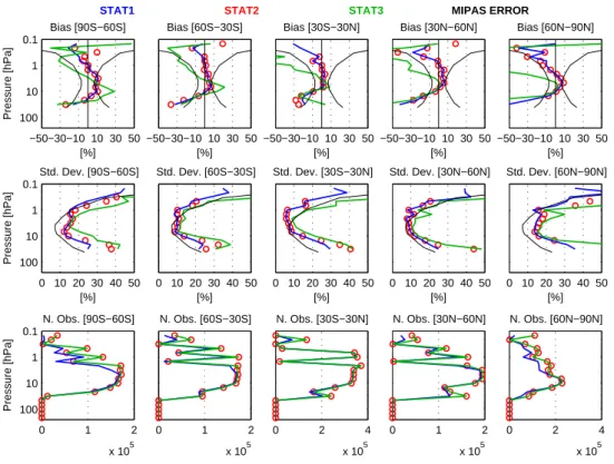
Interactive Discussion the bias and standard deviation for three comparisons: (1) MIPAS assimilated data

against BASCOE (“stat1”), (2) all MIPAS data (i.e., including data rejected by the quality control filter) against BASCOE (“stat2”), and (3) all MIPAS data against the control run described in Sect. 4 (“stat3”). The statistics are calculated using the method described in Sect. 3.4. They are calculated for the period September–October 2003, five latitude

5

bands and 21 pressure layers. The figure also shows the number of observations used to compute the statistics, and the MIPAS total error for ozone (see Sect. 4). From Fig. 2, we can make several remarks:

– In the stratosphere, the number of data assimilated is generally similar to the

to-tal available observations, indicating that few observations are filtered out. Thus,

10

the bias and standard deviation of stat1 and stat2 are similar. Rejected data correspond to either observations at the tropopause and levels below in the tro-posphere, or to data at the South Pole during ozone hole conditions. In both these cases, the bias and standard deviation are generally lower when only assimilated MIPAS data (stat1) are considered.

15

– In the stratosphere, the bias and standard deviation between BASCOE and all

MIPAS data (stat2) are generally smaller than the O₃MIPAS total error. The bias in stat2 is generally not significant. For example, at 10 hPa, biases are within [−2, 3]%. There are two regions where BASCOE fails to reproduce MIPAS within its uncertainty. Around 0.5 hPa, MIPAS is underestimated by BASCOE with a

20

significant bias of around 20% (see the later discussion on the analyses around the 0.5 hPa level). The second region where BASCOE presents a significant bias against MIPAS is at the South Pole during ozone hole conditions. For example, BASCOE overestimates MIPAS around 13% at 100 hPa. The standard deviation is also high, around 40% in the South Pole lower stratosphere. However, in these

25

cases, absolute differences might be a better estimator of the BASCOE quality since observed ozone amounts can be close to zero. The ozone hole represen-tation by BASCOE is further discussed in Sect. 5.2.

ACPD

Full Screen / Esc

Printer-friendly Version

Interactive Discussion

– BASCOE analyses values at the tropopause and levels below are very different

from the observations. This is due to the absence of tropospheric processes in the BASCOE CTM.

– The statistics from the analyses and the control run (stat3) are similar for levels

above 10 hPa. For levels below 50 hPa, biases from the analyses are smaller by

5

a few percent with respect to the control run. No significant differences can be seen in the standard deviation for levels below 10 hPa outside the South Pole. For levels above 10 hPa, the model is already within the error bars of MIPAS and the impact of the observations is small. For example, at 10 hPa in the Tropics the bias between MIPAS and the control run is around 6%, while the bias for

10

the same comparison against BASCOE (stat2) is around 2%. At the South Pole, however, the analyses show a clear benefit from data assimilation. For example, assimilation reduces the bias by 35% at 100 hPa. Between the lower stratosphere and the tropopause, a clear benefit from data assimilation is also seen in the bias and the standard deviation statistics.

15

In order to assess the temporal consistency of the BASCOE analyses, we plot in Fig. 3 the time series of the bias and the standard deviation of the differences be-tween BASCOE and MIPAS (stat2) for three pressure layers, five latitude bands and the entire twenty-one months of assimilation. Around the ozone maximum, between 8 and 12 hPa, the statistics are stable in time except for the standard deviation at the

20

winter Poles (e.g. we observe a maximum of 20% for the standard deviation in July). For all other latitudes and time periods at levels around the ozone maximum, the bias and standard deviation of the differences are not significant. At higher levels, between 0.6 and 1.8 hPa, BASCOE underestimates MIPAS, as discussed above. For levels be-tween 82 and 121 hPa, the bias and standard deviation are generally consistent in time

25

except at the Tropics and during the ozone hole period. In general, the statistics show higher variability at the Poles and at the tropical tropopause, two regions that can have a strong dynamical barrier. Increasing the resolution of BASCOE would likely reduce

ACPD

Full Screen / Esc

Printer-friendly Version

Interactive Discussion the bias and standard deviation, as discussed byStrahan and Polansky(2006).

We now consider the underestimation of MIPAS data by BASCOE at levels around 0.5 hPa, Fig. 4 shows the bias between MIPAS and BASCOE (stat2), and MIPAS and the control run (stat3). For this plot, we show the statistics for MIPAS nighttime and daytime data separately. The main differences between the daytime and nighttime

5

statistics occur around 0.5 hPa and levels above, where there is significant bias be-tween BASCOE and MIPAS. The control run shows the same behaviour, with a bias slightly higher than that for the analyses. This suggests the bias comes from the model, unlike stated inErrera et al.(2007) who mentioned a potential problem in the MIPAS observations. We suggest that this low bias is related to photolysis calculations in

BAS-10

COE, a bias that cannot be reduced by the assimilation. The 0.5 hPa level is close to the third pressure layer of BASCOE, which is close to the model lid. Hence, improv-ing the photolysis calculations at these levels would require addimprov-ing extra model layers above 0.1 hPa; changes that are not currently planned.

5.2 BASCOE vs. independent observations

15

To validate the analyses, we compare them against independent observations from HALOE and POAM-III. Figure 5 shows the bias and standard deviation of the differ-ences between BASCOE and, respectively, independent observations from HALOE and POAM-III, for the period September–October 2003. This period is representa-tive of the 21 months considered here, except for the lower South Pole stratosphere.

20

We recall that HALOE ozone errors are about 11% at 0.1 hPa, 5% between 1 and 30 hPa and gradually increase to 30% at 100 hPa (Br ¨uhl et al.,1996). POAM-III errors are below 5% throughout the polar stratosphere (Randall et al., 2003). In the middle stratosphere, between 2 and 50 hPa, and outside ozone hole conditions, the agree-ment between BASCOE and independent data from HALOE and POAM-III is generally

25

within HALOE and POAM-III uncertainties, i.e., bias and standard deviation are both lower than 5%. Between 50 and 100 hPa, the bias remains below 10% but the standard deviation increases to 90% at the Tropics and 20% at the other latitude bands (Fig. 5).

ACPD

Full Screen / Esc

Printer-friendly Version

Interactive Discussion Because aerosol and cirrus clouds at levels below 120 hPa can seriously affect HALOE

data, it is better to assess the quality of BASCOE analyses against other datasets less affected by Mie scattering, e.g. ozonesondes. This was done in the ASSET ozone intercomparison study (Geer et al.,2006). In that work it was shown that for levels be-low 100 hPa, BASCOE underestimates ozonesondes. For levels bebe-low 100 hPa at the

5

Tropics and levels below 200 hPa in the Extra-tropics, this underestimation is around 50%. This is due to the fact that BASCOE is not designed for the troposphere, does not include a proper parameterization of troposphere-stratosphere exchange, and is not tuned to adjust tropospheric ozone to more realistic values (e.g. from climatology). Above 2 hPa, the bias increases and is maximum around 0.7 hPa. The highest bias

10

is found at the Tropics where BASCOE underestimates HALOE by 11%. As mentioned in Sect. 5.1, this is probably due to the set-up of the photolysis rate calculations. While significant, this bias is much smaller than the bias between BASCOE and MIPAS. This comfirms the probable role of photolysis in the discrepancy since the local time of measurement between MIPAS and HALOE is different. At twilight (HALOE), the impact

15

of the photolysis rate calculation is less important on the ozone chemistry than during daytime (MIPAS). Above 0.5 hPa, the standard deviation increases slightly, reflecting the increased variability in observed ozone due to its diurnal cycle at these levels.

During the 2003 ozone hole the bias between BASCOE and independent data is significant. The bias between BASCOE and POAM-III is around 100% at 100 hPa.

20

However, the amount of ozone is so low that relative differences are no longer mean-ingful. In Fig. 6 we show a time series of POAM-III ozone averaged over two days for SH occultations and the corresponding BASCOE analyses. Ozone amounts are expressed as number densities to focus on the ozone hole altitude range. In gen-eral, BASCOE ozone is close to POAM-III data. The 2003 ozone hole observed by

25

POAM-III is qualitatively well reproduced by BASCOE, in agreement withGeer et al.

(2006, see their Fig. 23) who show good agreement between BASCOE and ozoneson-des at altituozoneson-des representative of the 2003 ozone hole. Absolute differences between POAM-III and BASCOE are in the range [−6, −2] × 1011molec/cm3 between 30 and

ACPD

Full Screen / Esc

Printer-friendly Version

Interactive Discussion 100 hPa; standard deviations are lower than 3× 1011molec/cm3. With respect to

other assimilation systems (see, e.g.,Geer et al.,2006), the ozone hole reproduced by BASCOE is qualitatively good. Nevertheless, a more advanced PSC parameterization (e.g.,Chipperfield,1999;Lef ´evre et al.,1998) could improve the ozone hole represen-tation.

5

Ozone analyses during the 2002 ozone hole overestimate POAM-III: this is the only period where BASCOE disagrees qualitatively with POAM-III. This is due to the lack of MIPAS data from 29 September to 11 October 2002, combined with the difficulty of BASCOE, due to its relatively low resolution, to capture realistically the dynamical evolution during the vortex split of 2002 (Newman and Nash,2005). For example,

aver-10

aged ozone observed by POAM-III at 68 hPa is around 1.5×1012molec/cm3while BAS-COE analyses for the same period show values around 3.5×1012molec/cm3. Based on these statistics, we conclude there is satisfactory agreement between BASCOE anal-yses and independent data except during the 2002 Antarctic ozone hole. Using these statistics, uncertainties of the BASCOE ozone analyses using HALOE and POAM-III

15

have been estimated (Table 1). No values are given for the 2002 Antarctic ozone hole since BASCOE values are qualitatively too far away from independent observations.

5.3 Estimation of differences between MIPAS and independent observations using BASCOE analyses

Due to temporal variability and geographical gradients in atmospheric composition,

20

temporal and spatial mismatches between two profile measurements can enhance dramatically the total error budget of their comparison and consequently preclude the intended determination of their bias and standard deviation. In order to reduce at best this contribution, classical satellite-to-satellite comparisons are usually limited to pairs of profiles selected through pre-defined co-location criteria. For example, in their

MI-25

PAS ozone validation paper,Cortesi et al. (2007, hereafter denoted C2007) adopted a maximum geographical distance of 300 km and a maximum time difference of 3 h

ACPD

Full Screen / Esc

Printer-friendly Version

Interactive Discussion between the MIPAS and HALOE observations, yielding for the period from July 2002 to

March 2004 a total of 141 profile pairs. The time and space interpolation capabilities of-fered by the data assimilation increase considerably the amount of co-located profiles that can be compared, since virtually all HALOE profiles can be used. The method consists in estimating differences between MIPAS data and independent

observa-5

tions using BASCOE as a transfer standard: (MIPAS-IndepObs)=(MIPAS-BASCOE)– (IndepObs-BASCOE), where IndepObs stand for HALOE and POAM-III.

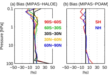
Differences between MIPAS and HALOE data using this method are shown in Fig. 7a for the year 2003 and for the five latitude bands. These results are based on 8311 HALOE profiles, compared to 141 co-located profiles found by C2007 in the validation

10

paper of MIPAS ozone, i.e., we use 60 times more profiles. The differences between MIPAS and HALOE data using BASCOE analyses as a transfer standard are compa-rable to the results found by C2007: we also find that MIPAS data are almost always higher than HALOE with less than +10% differences between 0.4 hPa and 60 hPa, and less than +5% differences between 3 hPa and 20 hPa. Where the analyses are of

15

poorer quality, i.e., near the model lid, in the troposphere and at the South Pole during the ozone hole, our method finds larger differences.

Differences between MIPAS and POAM-III data using BASCOE analyses as a trans-fer standard are shown in Fig. 7b for the year 2003 and for data from both hemispheres. These results are based on 7937 POAM-III profiles, compared with 1571 profiles in

20

C2007, i.e., we use around 5 times more profiles. Again, our results are similar to those obtained by C2007: we find a bias below ±5% between 0.5 hPa and 50 hPa. At 100 hPa, the differences between MIPAS and POAM-III found in C2007 increase to +12% in the NH and +15% in the SH. Again, this agrees with our results.

Differences between MIPAS and independent data from HALOE and POAM-III found

25

here are comparable to those found by classical validation methods (e.g. C2007) when the assimilation system is able to reproduce accurately the MIPAS observations. Val-ues found here reinforce significantly the representativeness of those published by C2007 (especially in the comparison against HALOE data) since a much larger variety

ACPD

Full Screen / Esc

Printer-friendly Version

Interactive Discussion of atmospheric states and of measurements conditions are taken into account in the

statistics presented in this paper.

6 Nitrogen dioxide results

In order to introduce the state of NO₂during the assimilation period, we show in Fig. 8 the time series of NOx derived from HALOE sunrise observations and the monitored

5

BASCOE analyses. The agreement between HALOE and BASCOE NOxdata is quali-tatively good except at the South Pole for two periods of time where HALOE observed relatively high NOxconcentrations. These periods occur in August 2003 and in Decem-ber 2003. These periods correspond to enhancement of NOx by Energetic Particles Precipitation (EPP,Randall et al.,2007). The first period corresponds to mesospheric

10

NO_x production by precipitating electron of medium energy (Funke et al.,2005). The second period corresponds to mesospheric-stratospheric NOx production due to So-lar Proton Events (SPEs) that took place from the end of October until mid November 2003 around Halloween (L ´opez-Puertas et al.,2005). The reason why BASCOE fails to reproduce these high NOxvalues is due to the fact that: (1) the production of NOxby

15

EPP is not modelled in BASCOE, and (2) MIPAS high NO2values are rejected by the quality control filter. We discuss below how these special events influence the quality of the NO2BASCOE analyses.

6.1 BASCOE vs. MIPAS

As for O3 (Fig. 1), Fig. 9 shows the zonal mean of NO2 observed by MIPAS and the

20

corresponding analyses on 6 October 2003. In order to separate daytime and nighttime observations, the zonal mean is given for the ascending and descending phases of the satellite. Qualitatively, the agreement between MIPAS and BASCOE is good for both phases. The bias and standard deviation between assimilated MIPAS data and BAS-COE analyses are given in Fig. 10 for MIPAS nighttime data. As for O3, we presents

ACPD

Full Screen / Esc

Printer-friendly Version

Interactive Discussion the statistics for the comparison between: (1) MIPAS assimilated data and BASCOE

(“stat1n”, where n stands for nighttime), (2) MIPAS all data and BASCOE (“stat2n”) and (3) MIPAS all data and the control run (“stat3n”). Here, we focus on a period where NOx is not influenced by any EPP events, between 1 and 24 October 2003. The number of MIPAS observations per pressure range and latitude band is also plotted. We can

5

make some remarks about Fig. 10:

– Except at the Poles, almost all nighttime observations are assimilated and there

is little difference between stat1n and stat2n. At the North Pole, around 40% of the observations are rejected above 3 hPa but bias and standard deviation be-tween stat1n and stat2n remain close; differences are visible only in the standard

10

deviation above 68 hPa. A similar behaviour is found at the South Pole where differences between the two statistics are visible above 0.5 hPa for the bias and 1 hPa for the standard deviation. Hence, rejected data are filtered out due to their variability not because they correspond to conditions that are not modelled; exactly the property that we expect from our data filter.

15

– For levels above 10 hPa outside the Polar Regions, BASCOE agrees in general

with MIPAS (stat2n) within the MIPAS total error. For levels below 10 hPa, the differences are significant. This is probably due to the set-up of sulphate aerosols in BASCOE that influence NOxin this altitude region. Nevertheless, the amounts of NO₂ become very small below 10 hPa, which makes the differences less

sig-20

nificant. Moreover, we did not take into account the error generated by the spatial interpolation and the time-lag between the observations and the model (maxi-mum 15 min), which can be significant due to the NO₂diurnal cycle (see Sect. 4). We thus conclude that BASCOE NO2is in good agreement with MIPAS NO2 be-tween 60◦S and 60◦N. At the Polar Regions, the agreement between BASCOE

25

and MIPAS is qualitatively poorer. While biases are generally not significant, the standard deviation is always higher than the total error, around 10% higher at the NO2peak (around 5 hPa). We suggest that the low resolution of BASCOE, which

ACPD

Full Screen / Esc

Printer-friendly Version

Interactive Discussion does not allow a strong barrier at the vortex edge, is the origin of this problem.

– For NO₂, a clear improvement is shown when one compares MIPAS against BAS-COE (stat2) instead of the control run (stat3). This is even clearer when looking at statistics above 10 hPa. This illustrates the benefit of assimilating NO2 obser-vations.

5

Similar conclusions can be drawn from statistics using MIPAS daytime observations, for which most observations are rejected above 1 hPa. This is due to the relatively low amount of daytime NO₂above that level (see Fig. 9b). On the other hand, even if these data are not filtered out, NO2 daytime errors are much larger than the background errors, and thus NO2daytime data have little influence on the final analyses.

10

Time series of the bias and standard deviation for stat2n are given in Fig. 11 for two pressure ranges and the five latitude bands. Outside the period/region of perturbed NOx, the bias is generally in the range [−1,7]% and [−15,7]% at around 3 hPa and 10 hPa, respectively. The corresponding standard deviation is below 15% and 20%, respectively. Taking into account the MIPAS total error and the fact that no error of

15

representativeness is included, we find these values acceptable. During perturbed NOx periods, the bias and standard deviation can be very high, e.g., 50%. This corresponds to the South Pole and the SH mid-latitudes between June and October 2003, and to the North Pole and NH mid-latitudes after the end of October 2003. For these cases, BASCOE underestimates MIPAS NO₂.

20

On the other hand, from June until August at 10 hPa and during June at 3 hPa, BAS-COE overestimates MIPAS NO2 at SH mid-latitudes with a maximum bias of around −30% and −15%, respectively (this was not revealed by the statistics shown in Fig. 10). This period corresponds to the South Polar Vortex, where values of O3and N2O, which drive NO2production, are very low. Since the model resolution does not allow a vortex

25

as isolated as it should be, BASCOE NO2 values are higher than the observations. This overestimation does not appear in the statistics at [60◦S–90◦S] because MIPAS observes the NOx perturbation by EPP at these latitudes. Thus, as for O3, BASCOE

ACPD

Full Screen / Esc

Printer-friendly Version

Interactive Discussion tends to overestimate NO₂in the Antarctic vortex during winter, likely due to the coarse

horizontal resolution of the model.

To conclude this subsection, outside the period when stratospheric NOxis perturbed, or outside the polar vortex, the assimilation performs well and BASCOE is able to reproduce the MIPAS data within its uncertainties.

5

6.2 BASCOE vs. independent observations

HALOE and POAM-III data have been monitored by BASCOE during the assimilation of MIPAS data. Time series of NO₂ observed by POAM-III at the South Pole and the monitoring analyses are given in Fig. 12 (see Fig. 8 for the analogous comparison between HALOE NOx and BASCOE NOx). Also indicated is the measurement mode,

10

local sunrise (SR) or local sunset (SS). NO₂ time series show a seasonal cycle with relatively low NO2 during the SH winter (June–August) and higher values during SH summer (December–February). The NH time series also exhibits such a cycle (not shown). Low winter NO₂is due to the presence of the polar vortex barrier which makes it difficult for N2O, the NO2 source gas, to reach the Pole. Moreover, during sunrise,

15

NO increases rapidly while NO2decreases and most of the NOxis thus in the form of NO (Randall et al., 2007). Conversely, during sunset observations, NO_x has relatively higher concentrations of NO₂. Thus, the switch of the occultation mode of POAM-III around the Equinox (see Sect. 3.3) increases the seasonal variation of NO2 given by the instrument.

20

BASCOE also exhibits this seasonal variation, in good qualitative agreement with the POAM-III data. From July to October 2003, POAM-III observes a thin tongue of relatively high NO2 descending from 2 to 10 hPa. This is the signature of the EPP event discussed above. The effects of the EPP are more apparent in the HALOE observations than in the POAM-III observations (see Fig. 8). The reasons for this are:

25

(1) POAM-III observations throughout most of the winter are done at sunrise, a time where most of the NO_x is in the form of NO, and (2) no POAM-III observations are available above 2 hPa. This explains why the enhanced level of NO2is not significantly

ACPD

Full Screen / Esc

Printer-friendly Version

Interactive Discussion higher than the background level. The tongue of relatively high NO₂is not reproduced

by BASCOE for the reasons discussed above.

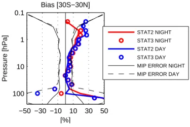
The bias and standard deviation between BASCOE and independent observations from HALOE (NO_x) and POAM-III (NO₂) are given in Fig. 13. Comparison with HALOE is done for a period where stratospheric NOx was not perturbed by EPP production,

5

i.e. from August 2002 until March 2004, excluding the periods May–August 2003 and the period of the Halloween SPE. During this period, the bias between HALOE and BASCOE is generally below ±10% (in magnitude) in the pressure range 1–10 hPa, where the NOxmixing ratio is maximum (Fig. 8). The standard deviation is minimum at the NO_x maximum (around 5 hPa) with values below or close to 10%. Below 10 hPa,

10

we provide the bias and standard deviation in volume mixing ratio, since the amount of NO2 becomes relatively low. Around 30 hPa, BASCOE overestimates HALOE and we find that the bias and standard deviation do not exceed −0.8±0.8 ppbv. Consid-ering the HALOE errors, which are between 10 and 15% in the middle stratosphere (Gordley et al.,1996), we find no significant bias between the BASCOE analyses and

15

HALOE data.

For reasons given above, comparisons against POAM-III in Fig. 13 are only done during summer, a time when the amount of observed NO2 is significant. This cor-responds to May–August 2003 for the NH comparison and to November–February 2003/2004 for the SH comparison (which is relatively similar to the statistics based on

20

November–February 2002/2003). The bias between BASCOE and POAM-III is higher than that between BASCOE and HALOE, being around 10% at the NO2peak (10 hPa, see Fig. 12).

Maximum bias is observed in the SH at 3 hPa (22%). The standard deviation is always below 15%. Based on POAM-III uncertainties (typically below 12%), this

sug-25

gests a significant bias above 5 hPa in both hemispheres. Below that level, no sig-nificant bias between BASCOE NO2 analyses and POAM-III NO2observations is ob-served.

stan-ACPD

Full Screen / Esc

Printer-friendly Version

Interactive Discussion dard deviations against HALOE. POAM-III data were not used to build this table since

it is difficult to interpret disagreements between the differences BASCOE-POAM-III and BASCOE-HALOE. We also only consider periods when the stratosphere is unper-turbed by EPP events, meaning that this table is not valid either during the SH 2003 winter or during the Halloween 2003 SPE.

5

6.3 Estimation of differences between MIPAS and independent observations using BASCOE analyses

Using BASCOE as a transfer standard (see Sect. 5.3), we estimate the difference be-tween MIPAS and independent observations from HALOE and POAM-III. In the pres-sure range 2–20 hPa, differences between MIPAS and HALOE are between ±13%

10

depending on the latitude band and the pressure level (Fig. 14a). Again, this compari-son adresses a period when stratospheric NOxwas not perturbed by EPP production. The validation study of MIPAS NO2 performed by Wetzel et al. (2007, hereafter de-noted W2007) found that MIPAS was high with respect to HALOE over the Antarctic, the southern mid-latitudes and the northern mid-latitudes. For these regions, our

re-15

sults agree with W2007. W2007 find that over the Arctic, MIPAS is low with respect to HALOE. This is not the case here, but the bias over the Arctic is lower than for other latitude bands for levels below 3 hPa. (Note that W2007 do not provide any compari-son between MIPAS and HALOE for the Tropics.) Excluding the Tropics, and between 2 and 10 hPa, the highest bias between MIPAS and HALOE found by W2007 is +20%

20

at 2 hPa in the middle latitudes for both hemispheres, and the lowest bias is −5% at 10 hPa over the Arctic. In general, our values are 5% higher than those found by W2007. We remark that W2007 find 260 HALOE co-located profiles, while we base our results on 6000 HALOE profiles.

Differences between MIPAS NO2 and POAM-III NO2 using BASCOE as a transfer

25

standard are given in Fig. 14b. We only provide comparisons for POAM-III sunset data for both hemispheres (as in Fig. 13b), i.e., a NH comparison for May–August 2003 and a SH comparison for November–February 2003/2004. Figure 10 suggests

ACPD

Full Screen / Esc

Printer-friendly Version

Interactive Discussion that MIPAS underestimates POAM-III between [−15,−6]%. W2007 estimate the

differ-ences between MIPAS and POAM-III for different periods of time. Two of the periods they choose are close in time to our choice of period: (1) April–June 2003 for NH co-locations; (2) October–December for SH co-locations (see Fig. 11 in W2007). For these cases, they find 36 and 125 co-located profiles, respectively, which have to be

com-5

pared with 605 and 651 profiles in our case. Differences between MIPAS and POAM-III found here agree with the values from W2007 for NH data: W2007 found MIPAS to be relatively low compared to POAM-III, between [−15,−10]% for levels above 10 hPa. For SH data, W2007 found that the bias between MIPAS and POAM-III is negative (−10%) at 3 hPa; they found a positive bias of +15% at 10 hPa. For these two cases, W2007

10

find that MIPAS and POAM-III agree within their combined errors. The differences be-tween MIPAS and POAM-III found here also agree within the combined errors of the two instruments. In the pressure range 3–10 hPa, the transfer standard method gives differences between instruments in agreement with those given by classical validation methods (e.g. W2007). Moreover, the transfer standard method brings together all the

15

HALOE and POAM-III data, extending the W2007 conclusions to a much larger variety of atmospheric states and measurement conditions.

7 Conclusions

In this paper we evaluate the performance of BASCOE ozone and nitrogen dioxide analyses produced by assimilation of ENVISAT MIPAS data. Although such data had

20

already been assimilated before, previous studies focussed on relatively short assim-ilation periods, typically a few months. In contrast, the assimassim-ilation period addressed by our study covers the entire 21 months (July 2002–March 2004) during which MIPAS operated at its nominal resolution. As well as providing an extended assimilation period (particularly for NO2), the analyses are evaluated by monitoring independent data from

25

HALOE and POAM-III. A seven-month free model run of the BASCOE CTM, starting in May 2003, is used as a control run to evaluate the benefit of the assimilation. Finally,

ACPD

Full Screen / Esc

Printer-friendly Version

Interactive Discussion BASCOE analyses are used to estimate differences between MIPAS data and HALOE

and POAM-III data.

O3 analyses are found to agree with MIPAS ozone data within the MIPAS errors. Comparison between the analyses and a free model run shows that the benefit of the assimilation is significant during the Antarctic ozone hole and in the lower stratosphere.

5

In other regions, the free model run agrees with the MIPAS data within the MIPAS er-ror bars; thus, while the difference against MIPAS is reduced by the assimilation, this does not provide significant improvement over the free model run. The gain from the assimilation is observed in regions where the model is known to have deficiencies. Comparison against independent data from HALOE and POAM-III shows that the

anal-10

yses are within the instrumental errors of the independent data. Using BASCOE ozone analyses as a transfer standard, estimates of the bias between MIPAS and HALOE, and MIPAS and POAM-III generally agree with values deduced by the classical valida-tion approaches which limit the comparisons to direct geographical co-locavalida-tion of the measurements. The main advantage of our method is that it increases the number

15

of correlative independent data used to validate MIPAS data; it thus extends and rein-forces the classical validation results, as a much larger variety of atmospheric states and of measurement conditions are taken into account.

The behaviour of the NO2 analyses is more difficult to interpret because during part of the assimilation period, the stratosphere was perturbed by NO_xproduction from

En-20

ergetic Particles Precipitation (EPP) events. Nevertheless, during the periods of unper-turbed stratospheric NOx, and around the NO2maximum (1–10 hPa), BASCOE is able to reproduce MIPAS daytime and nighttime data within the MIPAS errors. Comparison of BASCOE NO2 analyses with HALOE and POAM-III independent NO2 data shows the former to be qualitatively good (within the instrumental errors of the independent

25

data) outside the time period and region perturbed by EPP events. Differences be-tween MIPAS NO2data and independent HALOE and POAM-III NO2data are derived using BASCOE analyses; they agree with results from the classical method limited to co-located measurements only. As for ozone, this extends and reinforces previous

ACPD

Full Screen / Esc

Printer-friendly Version

Interactive Discussion results on the validity of the MIPAS data.

This study has revealed several weaknesses in the model, or in the set-up of the system that can degrade the analyses: (1) the model resolution is too coarse to de-scribe accurately dynamical barriers like the tropical surf zone or the Polar Vortex; this problem can be solved by increasing the horizontal resolution of the model. (2) The

5

online data filter rejects most of the MIPAS NO2observations during EPP events; bet-ter formulations of this filbet-ter, or off-line filbet-tering of the observations, would alleviate this. A parametrization describing the effect of the EPP on NOx in the model would also improve the NO2 analyses. (3) It was found that ozone analyses around 0.5 hPa un-derestimate the observations (both assimilated and independent). This is likely due

10

to the formulation of the photolysis rate calculations and the fact that 0.5 hPa is close to the model lid (0.1 hPa). We plan to perform experiments to test this hypothesis by using ECMWF wind data posterior to 2006, when ECMWF raised the model top up to 0.01 hPa.

BASCOE O3 analyses will become available via the PROMOTE project

15

(http://www.gse-promote.org), while BASCOE NO2analyses and other analysed fields (the latter not yet validated) can be obtained on request by emailing the first author of this paper.

Acknowledgements. We thank M. Chipperfield for providing initial fields from the SLIMCAT

CTM; the POAM-III and HALOE teams for making their data available to us; and K. Hoppel for 20

helping to interpret the POAM-III data. Q. Errera, S. Chabrillat and J.-C. Lambert are supported by the Belgian Federal Science Policy in the framework of the BASCOE ProDEx project for QE and SC (PEA 90125) and the CINAMON ProDEx project for JCL (PEA C 15151).

References

Baier, F., Erbertseder, T., Morgenstern, O., Bittner, M., and Brasseur, G.: Assimilation of MIPAS 25

observations using a three-dimensional global chemistry-transport model, Q. J. Roy. Meteor. Soc., 131, 3529–3542, doi:10.1256/qj.05.92, 2005. 8011

ACPD

Full Screen / Esc

Printer-friendly Version

Interactive Discussion

Bhatt, P. P., Remsberg, E. E., Gordley, L. L., McInerney, J. M., Brackett, V. G., and Russell III, J. M.: An evaluation of the quality of Halogen Occultation Experiment ozone profiles in the lower stratosphere, J. Geophys. Res., 104, 9261–9276, doi:10.1029/1999JD900058, 1999.

8018

Bouttier, F. and Courtier, P.: Data assimilation concepts and methods, March 1999, in: Meteoro-5

logical Training Course Lecture Series, ECMWF, http://www.ecmwf.int/newsevents/training/

rcourse notes/DATA ASSIMILATION/ASSIM CONCEPTS/Assim concepts.html, 2002.8015

Br ¨uhl, C., Drayson, S. R., Russell, J. M., Crutzen, P. J., McInerney, J. M., Purcell, P. N., Claude, H., Gernandt, H., McGee, T. J., McDermid, I. S., and Gunson, M. R.: Halogen Occultation Experiment ozone channel validation, J. Geophys. Res., 101, 10 217–10 240, doi:10.1029/ 10

95JD02031, 1996. 8018,8024

Chipperfield, M. P.: Multiannual simulations with a three–dimensional chemical transport model, J. Geophys. Res., 103, 1781–1805, 1999. 8020,8026

Cortesi, U., Lambert, J. C., De Clercq, C., Bianchini, G., Blumenstock, T., Bracher, A., Castelli, E., Catoire, V., Chance, K. V., De Mazire, M., Demoulin, P., Godin-Beekmann, S., Jones, N., 15

Jucks, K., Keim, C., Kerzenmacher, T., Kuellmann, H., Kuttippurath, J., Iarlori, M., Liu, G. Y., Liu, Y., McDermid, I. S., Meijer, Y. J., Mencaraglia, F., Mikuteit, S., Oelhaf, H., Piccolo, C., Pirre, M., Raspollini, P., Ravegnani, F., Reburn, W. J., Redaelli, G., Remedios, J. J., Sembhi, H., Smale, D., Steck, T., Taddei, A., Varotsos, C., Vigouroux, C., Waterfall, A., Wetzel, G., and Wood, S.: Geophysical validation of MIPAS-ENVISAT operational ozone data, Atmos. 20

Chem. Phys., 7, 4807–4867, 2007,

http://www.atmos-chem-phys.net/7/4807/2007/. 8017,8026

Daerden, F., Larsen, N., Chabrillat, S., Errera, Q., Bonjean, S., Fonteyn, D., Hoppel, K., and Fromm, M.: A 3D-CTM with detailed online PSC-microphysics: analysis of the Antarctic winter 2003 by comparison with satellite observations, Atmos. Chem. Phys., 7, 1755–1772, 25

2007,

http://www.atmos-chem-phys.net/7/1755/2007/. 8013,8014

Damian, V., Sandu, A., Damian, M., Potra, F., and Carmichael, G.: The Kinetic PreProcessor KPP – A Software Environment for Solving Chemical Kinetics, Comput. Chem. Eng., 26, 1567–1579, 2002. 8013

30

Dethof, A.: Assimilation of ozone retrievals from the MIPAS instrument on board ENVISAT, Technical Memorandum 428, ECMWF, Reading, UK, 2003.8011