HAL Id: hal-00678680
https://hal.archives-ouvertes.fr/hal-00678680
Submitted on 13 Mar 2012HAL is a multi-disciplinary open access
archive for the deposit and dissemination of sci-entific research documents, whether they are pub-lished or not. The documents may come from
L’archive ouverte pluridisciplinaire HAL, est destinée au dépôt et à la diffusion de documents scientifiques de niveau recherche, publiés ou non, émanant des établissements d’enseignement et de
Tiling Surfaces with M-Tiles: a Topological Framework
with Applications
Jean-Marie Favreau, Thibault Marzais, Yan Gérard, Vincent Barra
To cite this version:
Jean-Marie Favreau, Thibault Marzais, Yan Gérard, Vincent Barra. Tiling Surfaces with M-Tiles: a Topological Framework with Applications. 2009. �hal-00678680�
Tiling Surfaces with M-Tiles: a
Topological Framework with
Applications
Jean-Marie Favreau
1Thibault Marzais
2Yan G´erard
2Vincent Barra
1Research Report LIMOS/RR-09-08 18 novembre 2009
– LIMOS, CNRS, Univ. Blaise Pascal, 63173 Aubi`ere cedex, France
– Univ. Clermont 1, LAIC, IUT Dpt Infor-matique, F-63172 Aubi`ere, France
Abstract
We present a framework to describe tiling of triangulated surfaces, possibly with boundaries. The M-tiles introduced by our framework may be home-omorphic to a disc or not, and capture both the tiles’ shape and the geo-metrical and non-trivial topological information of the original mesh. Some tiling algorithms using a cutting scheme are presented using this framework to describe each intermediate state of the cutting process. In particular, we use tiling with a unique tile homeomorphic to a disc to produce an effective computation of the polygonal schema, and to produce a quadrangulation of the original mesh with running time O(gn2
log n), where n is the number of vertices of the mesh, and g the genus. We show that this algorithm produces the minimal number m = 2g − 1 of quadrangles on a boundaryless mesh. Finally, we give some application results and variations on the algorithms. Keywords: Tiling framework, M-tiling, M-tile, cutting surfaces, quadran-gulation
R´esum´e
Nous pr´esentons un cadre pour d´ecrire le pavage de surfaces triangul´ees, ´eventuellement `a bord. Les M-tuiles introduites par notre cadre peuvent ˆetre hom´eomorphes ou non `a un disque, et capturent `a la fois la forme des tuiles, ainsi que les informations g´eom´etriques et topologiques non tri-viales du maillage original. Des algorithmes de pavage utilisant une approche d´ecoupage sont pr´esent´ees, nous profitons de ce cadre pour d´ecrire chaque ´etape interm´ediaire du processus de d´ecoupage. En particulier, nous utilisons un pavage par une unique tuile hom´eomorphe `a un disque pour produire une m´ethode effective du sch´ema poligonal, et pour introduire une quadrangula-tion du maillage original avec une complexit´e en temps en O(gn2
log n), o`u n est le nombre de sommets du maillage, et g le genre. Nous montrons qe cet algorithme produit le nombre minimal m = 2g − 1 de quadrangles sur un maillage sans bord. Enfin, nous pr´esentons quelques r´esultats applicatifs et variations sur les algorithmes.
Mots cl´es : Cadre de pavage, M-pavage, M-tuile, d´ecoupage de surfaces, quadrangulation
Acknowledgement / Remerciements
1
Introduction
Triangulated meshes are the most classical way to model a surface of R3
, whether they are generated from a 3D acquisition or in an abstract way. This kind of data structure can indeed describe 2-manifolds with or without boundaries, and with any topological configuration.
In this work, we present a framework to describe tilings of meshes, and intermediate data structures of the tiling processes. Tiling a surface is the process of partitioning this surface in regions called tiles. This partitioning may be produced by cutting the surface [10], i.e. by describing the boundaries of the tiles, or by performing a segmentation of the surface [16], i.e. by partitioning the surface.
Applications of such tiling are various, from Computer Graphics (Texture Mapping) to CAD (reconstruction of parameterized surfaces) or simulation (for instance by finite elements on quadrangulated surfaces [2]).
The tiling methods are driven by the application, and may use some topological [18] or geometrical information [19]. They also may impose some properties on the produced tiles, like their shape [8, 1], their topology [3] or their semantic properties [20]. Other methods are obviously mixing several of those caracteristics [6] to produce tilings suitable for the application.
The originality of our approach is to set up a framework to capture geo-metrical, non-trivial topological information and tiles’ shape manipulated by the tiling methods. In a first part, we will describe the tile and tiling frame-work, then we will expose some algorithms based on cutting processes to pro-duce a unique tile from any 2-manifold non homeomorphic to a sphere. Next an algorithm to produce tiling with quadrangles will be proposed. Those tiling methods take into account both topological and geometrical properties of the surface, using cutting lengths as criterion. Finally, some experimental results are presented for each algorithm, and some variations on the distance caracterization are evoked to take into account information like the local curvature of the surface or the application needs.
2
Cells and Tilings
2.1
Initial Mesh
Definition 1 A 2-mesh M is a 2-manifold simplicial 2-complex (with or without boundaries). In other words M is a union of 0-simplices called ver-tices, of 1-simplices called edges and of 2-simplices called triangles, and locally homeomorphic to a disc or a half disc.
If the definition of a tiling of a 2-mesh is rather straightforward, the process we used to compute such a tiling requires the introduction of a topo-logical framework that defines the cutting of a surface in a mathematical sense.
2.2
Topological Framework: a Notion of
2-m-cell
It is usual in Computer Graphics to consider cells which are simplices or con-vex polyhedrons since they have a well-known structure with faces, edges and vertices. In this classical framework, a cell complex is a set of cells (namely of polyhedrons) satifying two conditions: (i) any face (of any dimension) of a cell is included in the complex and (ii) the intersection of two cells is a cell. It follows from condition (i) that for any cell of dimension k, its sub-cells of dimension k − 1 cover its boundary. The class of cells used in this framework, the polyedral cells, is nevertheless not sufficient for our purpose (neither are CW-complexes [25]). We indeed need cells which are not necessarily homeo-morphic to a disc (we do not exclude for instance cylindric cells, as described in section 2.4) but detailing such a topological framework in this paper would require a lot of work and is not the purpose here.
A solution could be to benefit from the theoretical framework provided by abstract cellular complexes [17]. An abstract cellular complex is a set of abstract elements called cells, each one having a dimension, and provided by a relation of partial order to describe which cell is the boundary of another. The notion of dimension becomes straightforward as well as the boundary relation if cells are instantiated as compact connex manifolds. It means that the framework of abstract cellular complexes allows the algorithms to deal with compact connex manifolds (with boundaries). Conditions (i) and (ii) must however be considered for defining the notion of m-cellular complex (m stands for manifold) of a dimension less than two:
Definition 2 An m-cellular complex C (of dimension less than two) is a set of m-cells with the following properties:
• (dimension condition) 2-m-cells are compact connex 2-manifolds with
boundary, 1-m-cells are simple, closed or opened curves, and 0-m-cells are points.
• (boundary condition) The boundary of any i-m-cell should be covered
by an (i − 1)-sub-complex, 1 ≤ i ≤ 2.
• (coherence condition) The intersection of two cells should be an
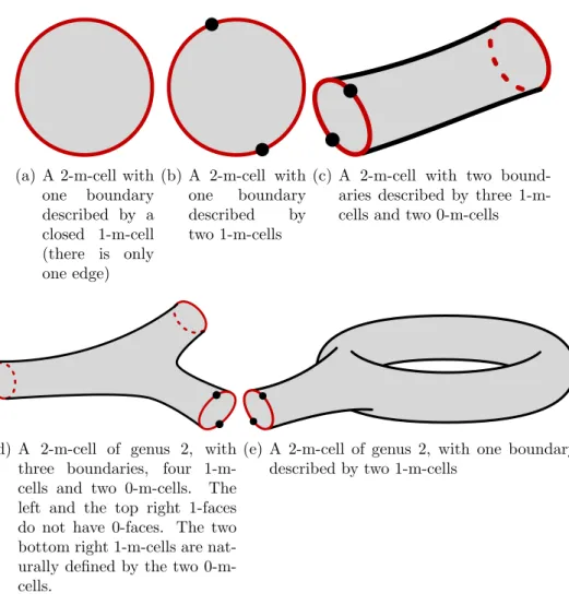
(a) A 2-m-cell with one boundary described by a closed 1-m-cell (there is only one edge) (b) A 2-m-cell with one boundary described by two 1-m-cells
(c) A 2-m-cell with two bound-aries described by three 1-m-cells and two 0-m-1-m-cells
(d) A 2-m-cell of genus 2, with three boundaries, four 1-m-cells and two 0-m-1-m-cells. The left and the top right 1-faces do not have 0-faces. The two bottom right 1-m-cells are nat-urally defined by the two 0-m-cells.
(e) A 2-m-cell of genus 2, with one boundary described by two 1-m-cells
Figure 1: Some 2-m-cells. Their boundaries are described by a structure of 1-complexes.
The second item claims that 2-m-cells have boundaries defined by a struc-ture of a non-empty 1-complex (Figure 1). It means that each boundary is decomposed as an alternate sequence of 1-m-cells and 0-m-cells that we call its edges (1-faces) and its vertices (0-faces). Generally speaking, we call faces of an i-m-cell the (i − 1)-m-cells, included on the boundary, 1 ≤ i ≤ 2. The
body of an i-m-cell is this i-m-cell minus its boundary.
Non degenerated polyhedrons in dimension 2 are 2-m-cells. In the follow-ing, a polygon with n edges will be called an n-polygon.
As 2-m-cells are 2-manifolds, they have their own topology. The interior of an i-m-cell is defined as the entirety less its (i − 1)-faces.
C
M
F
F(C )
0
0
Figure 2: An M-tile described by the 2-m-cell 1(c) and an embedding F on a 2-mesh of genus 2.
2.3
Tiles and Tilings
An M-tile is defined by embedding a 2-m-cell in a 2-mesh.
Definition 3 Let F be the set of embeddings F : C −→ M of a 2-m-cell C in a 2-mesh M verifying the following properties:
• F is continuous.
• Let v be a vertex of C. Then F (v) is a 0-simplex of M.
• Let e be an edge of C. Then F (e) is a set of 1-simplexes of M. • Let b be the body of C. Then F (b) is a set of 2-simplexes of M. • An embedding is usually injective but we accept in our framework that
two vertices or two edges may have the same image: F should only be injective on the interior of C (more precisely, we authorize vertices of the boundary of C to collapse: two such vertices can have the same image by F . We assume also that if two points x and y of the interior of edges e and e′ have the same image, then F (e) = F (e′)).
F, F′ ∈ F are said to be equivalent if and only if for any face, edge or
vertices X of C, F (X) = F′(X). The equivalence classes of this relation are
called M-tiles. For the sake of simplicity, an M -tile is denoted by one of its instance (C, M, F ).
An M-tile (C, M, F ) is fully described by the 2-m-cell C and the image by F of C, its edges and vertices. Choosing some images for each vertex, edge and 2-m-cell is however not sufficient to define an M-tile, because their topological consistency will not be guaranted (the topological consistency is related to the existence of such an F satisfying the conditions of Definition 3). When C is an n-polygon, the M-tile is a standard tile. Figure 2 shows an example of an M-tile.
M
F
F(C )
C
0 0C
1C
2F(C )
1F(C )
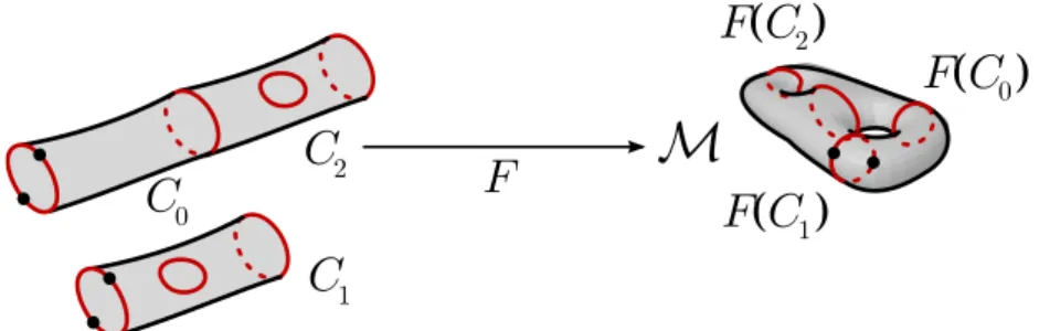
2Figure 3: A M-tiling (C, M, F ) of the 2-mesh M of Figure 2 by an m-cellular complex with three 2-m-cells
Definition 4 A M-tiling of a 2-mesh M by an m-cellular complex C is an equivalence class of embeddings F : C −→ M where:
• For all C 2-m-cell of C, F|C represents an M-tile.
• The restriction of F to the union of the interiors of the m-cells that
are not boundaries should be injective (covering the interior of m-cells is thus forbidden). We assume again that if two points x and y of the interior of edges e and e′ have the same image, then F (e) = F (e′) (this
condition avoids “T” shape junctions).
• F is surjective.
Two embeddings F and F′ are said to be equivalent if and only if for any
i-m-cell X of the m-cellular complex C, F (X) = F′(X).
As in the case of the M-tiles, a M-tiling is fully described by the m-cellular complex C and the images of each m-cell of C in M.
If the 2-m-cells of C are n-polygons, the M-tiling is a standard tiling of M. Figure 3 shows an example of a M-tiling.
2.4
Framework Justification
The M-tiles and M-tilings framework will be first used in section 3 to produce a single tile on arbitrary boundaryless 2-meshes, then in section 4 to produce quadrangulations.
This framework makes it possible to describe each step of the M-tiles generation, including the final M-tiles, that are homeomorphic to a disc, as standard tiles.
But this framework can also manipulate non-trivial M-tiles, and the in-formation carried out by the embedding (connection between tiles on the
(a) A pant, surface of genus 0 with 3 boundaries, each of them being described by a unique 1-face.
(b) A decomposition of a pant by three cylinders. Each cylinder has two boundaries, the first one with a unique 1-face, and the other with two 1-faces and two 0-faces.
Figure 4: A pant and a corresponding M-tiling with three cylinders. boundaries, and topological structure) may be used by applications to im-prove their description and mechanism.
Colin de Verdi`ere et al. [3] recently proposed an algorithm to decompose a surface into pants (Figure 4(a)), i.e. into surfaces of genus zero with three boundaries. This decomposition can be described by our framework, representing both the decomposition and the embedding between the 2-cells of genus zero with three boundaries and the original 2-mesh.
Using the precise description of boundaries, with 0-faces and 1-faces that M-tiles and M-tilings propose, each pant can be decomposed into three cylin-ders (Figure 4(b)). Each of those cylincylin-ders has two boundaries, the first one with a unique 1-face, and the other with two 1-faces and two 0-faces. Using an algorithm to build a tiling of 2-meshes by pants, we are able to produce a tiling by cylinders of any surface.
This example illustrates the large flexibility of our framework, that per-mits to describe various topological and geometrical segmentation methods, whilst describing also intermediate steps of the generation algorithms. In the next sections, we describe an iterative method to build a tiling of any 2-mesh with quadrangles, using first a tiling with a single tile.
3
Tiling a Mesh with a Single Tile
Let P be an n-polygon, and M a 2-mesh. Tiling M with a single tile T = (P, M, F ) is not completely straightforward if M is not homeomorphic to a disc. Thus, a practical approach is based on cutting the mesh into a disc.
3.1
Cutting and Tiling
The computation of cuttings is the core of the tiling process provided in this paper, thanks to the next lemma:
Lemma 1 A tiling T = (P, M, F ) of a 2-mesh M is equivalent to a set Γ of 1-faces of the mesh, the complement Γ of Γ in M being homeomorphic to a disc. Γ is called a cutting.
Proof Let T = (P, M, F ) be a tiling. Then images of the edges of P provide a cutting.
Let us now consider a cutting Γ on M with Γ homeomorphic to a disc. Tiling M by a unique tile T = (P, M, F ) can be constructed as follow:
• The image of the body of the 2-m-cell of P is defined as Γ ∪ B, where B is the boundary of the mesh.
• The image of the vertices V of P on M are defined by the set of vertices of Γ∪B. Using an extension by continuity of the homeomorphism from Γ ∪ B to the disc, the images of vertices in Γ ∪ B are on the boundary of the disc. They naturally define the vertices of the polygon.
• Each edge of P is also described by this homeomorphism.
The polygon generated from the cutting has at least as many vertices as the cutting. This number can however easily be reduced by removing the boundary of P whose image takes part in exactly two edges of Γ ∪ B (Figure 5). According to section 3.3, this reduction is not so insignificant.
In this paper, the 0-faces of M taking part in F (V ) are called multipoints. This definition naturally extends when F is the embedding associated to a general M-tiling with more than one M-tile, and with non-polygonal M-tiles.
3.2
Computing a Minimal Length Cutting
Now that we know how to obtain a tile from a cutting, we introduce the topological process for cutting a mesh into a disc.
Cutting a mesh into a disc is a topological process: the aim is to modify both the genus and the boundary cardinality until the homeomorphic con-dition is reached. Given a 2-mesh, there is no canonical solution for this cutting, and topologically equivalent cuttings may be roughly different when considered from other criterions. More particularly, if they are assessed with respect to their length, defined as the sum of the lengths of the 1-faces con-tained into Γ, Erickson and al. [10] showed that computing the length of the
F P F
M
M
P' 'Figure 5: An M-tile (P, M, F ) of a 2-mesh M. P is a polygon computed using the method described in the proof of Lemma 1. The M-tile (P′, M, F′)
has been obtained by removing vertices of P whose images take part in exactly two edges of Γ ∪ B.
minimum cutting of a 2-mesh is NP-hard. They also defined an effective method, using the Dijkstra algorithm [7], to compute a good approximation of the optimal cutting in polynomial complexity. The cutting method did not handle the simple case of meshes homeomorphic to a sphere. Using the 2-m-cell and M-tiling structures defined in section 2, this cutting method can be structured as an iterative algorithm that selects and cuts along a 1-path, and relies on the definition of valid 1-paths and valid 1-loops.
Definition 5
• A 1-path of a 2-mesh M is a list of n oriented edges s0, ..., sn−1 when
for each i = {0, ..., n − 2}, the terminal vertex of si is the initial vertex
of si+1.
• A 1-cycle of a 2-mesh M is a 1-path s0, ..., sn−1 where the initial vertex
of s0 is the terminal vertex of sn−1.
• A 1-path in M is valid according to an M-tile (C, M, F ) if it is the
image of a path p : [0, 1] → C by F (it avoids crossing the image of the boundary of C).
• A valid 1-path of (C, M, F ) between two different boundaries b1 and
b2 is a 1-path in M image of a path p : [0, 1] → C by F , with p(0) ∈ b1
M
b1 b2F
l m n o kC
Figure 6: An M-tile (C, M, F ) of a 2-mesh M. C is a 2-m-cell with two 1-cells b1 and b2. k is a trivial (separating) 1-loop, l is a non-valid 1-path, m
is a valid 1-path between b1 and b2, n is a valid non-trivial separating 1-loop,
and o is a non-separating 1-loop.
• A trivial 1-loop of (C, M, F ) is a 1-cycle in M image of a loop by F
and homotopic to a loop reduced to a point.
• A valid separating 1-loop (resp. non-separating 1-loop) of (C, M, F )
is a 1-cycle in M image of a loop by F that splits (resp. does not split)
C in two connected components.
Given these definitions (illustrated in Figure 6), the global cutting method is described in Algorithm 1, and the different steps are detailed in the fol-lowing subsections.
Data: a 2-mesh M non homeomorphic to a sphere T = (C, M, F ) is an M-tile initialized as M;
while the genus of C is not 0 do
Find c the shortest valid non-separating 1-loop of T ; Cut T according to c;
while the number of boundaries of C is not 1 do
Find c the shortest valid 1-path of T between two different boundaries;
Cut T according to c;
Algorithm 1: Global algorithm
3.2.1 Finding a non-Separating 1-loop
Given an M-tile T = (C, M, F ), and a distance d on edges of M, the short-est non-separating 1-loop is processed by first computing a list of basepoints, starting points of the potential 1-loops, then by computing the shortest cor-responding 1-loop.
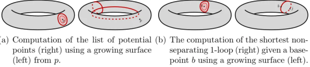
A list of potential basepoints is first computed using a growing surface. For this, a point p is selected from the interior of C. Triangles of the 2-mesh are then added as a growing surface, preserving the original connectivity and assuming that this growing surface is continually homeomorphic to a disc [14].
p p
(a) Computation of the list of potential points (right) using a growing surface (left) from p.
b b j
(b) The computation of the shortest non-separating 1-loop (right) given a base-point b using a growing surface (left). j is the junction point used to com-pute the final loop.
Figure 7: Two steps of the non-separating 1-loop computation. At the end of this growing process, some boundaries of the resulting surface are not boundaries of the M-tile. Corresponding paths on the original 2-mesh M can easily be computed. The points of these paths are the potential basepoints. In fact, a non-trivial 1-loop has to go through one of these points. Then for each potential basepoint p, the corresponding shortest non-separating loop is determined by growing a surface on the 2-mesh, with respect to the 2-m-cell, starting from p (Figure 7(a)). When two boundary parts of the growing surface join, the connected components of the comple-ment of the growing surface is computed. If there is only one connected com-ponent, the junction point j is included in the non-separating loop, built us-ing the two paths from p to j accordus-ing to the growus-ing process (Figure 7(b)). Otherwise, the growing surface joins at the junction point, and the growing process continues.
The globally shortest separating loop is the shortest of all the non-separating loops.
If no non-separating loop has been found for the first selected basepoint, there is no non-separating loop on the M-tile. Thus the genus of the M-tile is 0, stopping the first iterative process.
3.2.2 Cutting an M-tile
According to the definition of a valid 1-path c of (C, M, F ), there is a path p : [0, 1] → C such that F (p) = c. Cutting through this 1-path thus consists in explicitly defining each face of the 2-m-cell of the new M-tile. The body of the new 2-m-cell is identified as the body of the original 2-m-cell where p([0, 1]) has been removed. Vertices of the new 2-m-cell are defined by first defining the pre-vertices of the new 2-m-cell as the vertices of the original 2-m-cell plus the points contained both in p([0, 1]) and in the boundary of the 2-m-cell. The vertices of the new 2-m-cell are the pre-vertices, duplicated if they take part in p([0, 1]). The neighborhood of the twin vertices defined by the duplication is located on every side of the cutting path. Then the edges
vc vd vb va vc vd vb va vc vd ' ' '' ''
Figure 8: Cutting an M-tile according to a path. Left: an M-tile (grey region) with four edges (black lines), a cutting path (red line), and four pre-vertices (va, vb, vc and vd). Right: the resulting M-tile with vertices va, vb, and the
new twin vertices (v′
c, vc′′) and (v′d, vd′′).
of the new 2-m-cell are identified as the boundaries of the body between two vertices of the new 2-m-cell (Figure 8).
This cutting clearly defines a surjective mapping π from the new 2-m-cell to the original 2-m-cell, with F ◦ π = Fnew, where Fnew is the embedding
associated to the new M-tile. Figure 9 shows a diagram corresponding to the full iterative process described by Algorithm 1.
3.3
Measuring the Complexity with the Number of
Edges of the Polygon
The number of edges of the final polygon is a criterion to describe the com-plexity of a tiling. But Algorithm 1 does not constrain this number, it only focuses on the length of the paths, and another method has thus to be de-veloped to manage this criterion.
The number of edges of the final polygon does not depend only on the topology of the surface. Figure 10 illustrates non unicity of the number of edges of a tiling. Minimizing this number guarantees that the tiling structure only depends on the topology, the geometry of the surface only impacting on the location of the paths. Moreover, the multiple tiling process, described in section 4, depends on this single tiling, and the number of tiles is directly related to the number of edges of the original cutting. Finally, a cutting that does not consider the number of edges often produces edges with small lengths that are not good candidates for e.g. a parameterization of the surface, which is one of the potential applications proposed here (see 5.2). For that reason, we are looking for the minimal number of edges of a tiling.
C0 C1 C2 C3 C4 C5 M F0 F1 F2 F3 F4 F5 π 0 π 1 π 2 π 3 π 4
Figure 9: Diagram of the iterative process. (C0, M, F0) is the initial M-tile.
(Ci, M, Fi) is the M-tile computed at the i-st iteration of Algorithm 1, and
πi is the surjective mapping described by the cutting of an M-tile (see 3.2.2).
Figure 10: Two available tilings of a torus. Left: tiling with a 4-polygon. Right: tiling with a 6-polygon.
F(p(0))
1 F(p(1))1
(a) Projection of a tile (P, M, F )) on M.
(b) Projection after merging the F (p1(0)) and F (p1(1))
vertices according to the formal approach described at section.
(c) Projection after merging two other vertices.
b c
a d
(d) Projection after merging the last vertices. The tile is now composed of four edges. a a b d c d c b (e) Corresponding canonical polyg-onal schema.
Figure 11: Projection of a tile on a mesh, after merging steps according to the formal approach described at section 3.3.1.
3.3.1 Minimal Number of Edges
The algorithm described in paragraph 3 provides a unique polygonal tile T = (P, M, F ) from any 2-mesh, but the number of 1-faces is not constrained by the topology. By minimizing this number, we propose recovering the canonical polygonal schema of M, and thus to fully caracterize the topology of the surface [13].
As a formal approach, the minimal number of 1-faces can be computed using a non-optimal polygonal cutting, because the number of 1-faces of the polygon can iteratively be reduced. A 1-face f1, described by a path p1 :
[0, 1] → P , where F (p1(0)) 6= F (p1(1)), is first processed. According to the
cutting process, there is a unique 1-face f2 described by a path p2 : [0, 1] → P
and having F (p1) = F (p2). Both f1 and f2 are then removed by merging
p1(0) and p1(1), assuming that other paths such that (F (p1(0)) or F (p1(1))
are terminal vertices are distorted on the 2-mesh to keep their structure (Figure 11). Given an original 2-mesh with no boundary, this process allows all the 0-faces of the polygon to have the same image on the 2-mesh, and no more 1-face can be removed.
This configuration can also be obtained during the generation by mod-ifying the 1-path selection to use an already single basepoint. Algorithm 2 describes this cutting process, and allows the computation of a single multi-point b on the polygon:
Data: a 2-mesh M without boundary, non homeomorphic to a sphere T = (P, M, F ) is an M-tile initialized as M;
Find c the shortest valid non-separating 1-loop of T ; Cut T according to c;
Find c the shortest valid 1-path of T between the two different resulting boundaries, with p(0) = p(1) (where p = f (c));
Let b = p(0);
Cut T according to c;
while T is not homeomorphic to a disc do
Find c the shortest valid 1-path of T having p(0) = p(1) = b and which does not cut C in two connected components;
Cut T according to c;
Algorithm 2: Cutting with a single point.
Note that this method provides a natural computation of the canoni-cal polygonal schema 11(e), similarly to the method provided by Colin de Verdi`ere et al. [4] based on the computation of the shortest homotopical loop to a given one.
Because of the large number of 1-paths going through b, some mesh mod-ifications around b have to be applied on the original 2-mesh. A splitting process is introduced in section 4.2, to avoid tangent paths. For surfaces with large genus, these modifications can become consequentials.
3.3.2 Intermediate Cutting Method
An intermediate algorithm (Algorithm 3) has been designed to reduce but not minimize the number of multipoints. It is a modified version of the original algorithm, that minimizes the creation of multipoints during the 1-path computation process.
Data: a 2-mesh M non homeomorphic to a sphere T = (C, M, F ) is an M-tile initialized as M;
while the genus of C is not 0 do
Find c the shortest valid non-separating 1-loop of T ; Cut T according to c;
while the number of boundaries of C is not 1 do
Find c the shortest valid 1-path of T between two different boundaries minimizing the creation of multipoints; Cut T according to c;
Algorithm 3: Intermediate cutting method
cou-ple regions from a set of regions defined by the set of existing multipoints and the boundaries of C with no multipoint. If the selected regions are both multipoints, the 1-path definition is immediate. If only one of the two re-gions is a multipoint, a new multipoint has to be created on the other region. Finally, if the selected regions b0 and b1 are both boundaries without
mul-tipoints, a single multipoint is created if their images on M coincides, i.e. F (b0) = F (b1). Otherwise a multipoint is created on each boundary.
4
Tiling a Mesh with Multiple Tiles
Tiling a mesh with a single tile has numerous applications, e.g. in UV map-ping [23], where a single map has to be defined for the whole surface, and some examples of such cuttings will be presented in section 5. However, when considering applications such as surface parameterization, the shape or the number of edges of the tiles are essential criterions to describe the quality of the tiling. This section describes a multiple tiling method, based on the single tiling process.
4.1
From One to Several Tiles
Given a tiling T = (C, M, F ), where C is composed of a set of polygons, a tiling T = (C′, M, F′) with a single polygonal tile can be easily computed
by iteratively merging the tiles of C, preserving the genus at each step. The reverse construction, i.e. tiling with multiple polygonal tiles from a unique tile using a cutting process, is the natural approach described in this section. Starting from a tiling by a single tile T = (P, M, F ) of a 2-mesh M, as computed for instance by algorithm 1, 2 or 3, Algorithm 4 generates a tiling of M with multiple tiles:
Definition 6 A cutting 1-path of a tile T = (P, M, F ) of boundary b is a
1-path in M image of a path p : [0, 1] → P by F , with p(0) ∈ b and p(1) ∈ b,
Data: a 2-mesh M without boundary, non homeomorphic to a sphere T = (P, M, F ) is a tile computed with a method described in
section 3;
while T has to be cut do Select a 2-m-cell C in T ;
Find a cutting 1-path c of T in C; Cut C according to c;
Update T ;
Algorithm 4: Generic method for tiling by successive cuttings of a single tile.
The number of tiles only depends on the number of cutting steps. How-ever, the number of multipoints depends both on the number of multipoints of the original single tile and the cutting steps. In fact, each cutting step of the iterative process defined in Algorithm 4 may either keep unchanged the number of multipoints, or increase it. If p : [0, 1] → P is the path associated to the cutting 1-path, the evolution of the number of multipoints depends on the location of p(0) and p(1). If F (p(0)) and F (p(1)) are multipoints, there is no increase. On the other hand, if neither F (p(0)) nor F (p(1)) are multipoints, and if F (p(0)) 6= F (p(1)), the cutting process introduces two new multipoints. If only one of the two points F (p(0)) and F (p(1)) is a mul-tipoint, or if they are both multipoints and F (p(0)) = F (p(1)), the cutting process introduces a new multipoint.
Hence, if the number of multipoints has to be kept constant, then existing multipoints must be connected in the process.
4.2
Tiling with Quadrangles
Algorithms defined in section 3 produce a single polygonal tile with an even number of 1-faces. A tiling in quadrangles can now be obtained by following generic Algorithm 5 under the condition that each cutting step preserves next Q criterion:
Definition 7 An M-tile T verifies the Q criterion if the 2-m-cell associated to T is an even n-polygon, with n ≥ 4. A tiling T satisfies the Q criterion if and only if each of the tiles satisfies it.
It provides a final algorithm for computing a quadrangulation of M. The shortest 1-path preserving the Q criterion is selected by checking each of the potential 1-paths that preserve the Q criterion (Figure 12(a)). For each 0-face a of a given n-polygon, each of the valid 0-faces vi is checked
Data: a 2-mesh M without boundary, non homeomorphic to a sphere T = (P, M, F ) is a tile computed with a method described in
section 3;
while T contains a non 4-polygon tile do Select a non 4-polygon 2-m-cell C in T ;
Find the shortest cutting 1-path c of T in C that preserves the Q criterion;
Cut C according to c; Update T ;
Algorithm 5: Tiling by successive cuttings of a single tile.
7
7
8
6
(a) Left: a unsatisfactory cutting that does not preserve the Q cri-terion. Right: a suitable cutting.
12
12
a
v
0v
1v
2v
3 (b) Example of a 12-polygon. a is the selected 0-face, and the viare the potential extremities of the cutting path preserving the Q criterion.
Figure 12: Cutting an even polygon into two even polygons. The number of edges is indicated in the polygons.
(a) A hexagonal tile with six vertices a, b, c, d, e, f and a stuck cutting be-tween b and e.
(b) The 2-mesh after the unsticking process of the cutting between b and e.
Figure 13: Illustration of the unsticking process on a simple example: the path b-e crossing the surface does not have boundary points, except b and e. This cutting process can provide in some cases unsatisfying quadrangles as illustrated by Figure 13(a). An unsticking process described in Figure 14(b) is applied by refining the mesh around the unsatisfying boundary edges or vertices (new vertices and edges are introduced without changing the surface). Each boundary 0-face of a cutting path is unstuck by splitting the neighboring 0-faces (Figure 13(a)).
Erickson et al. [10] showed that the cutting produced by Algorithm 1 is a good approximation of the minimal cutting. Using the minimal length to produce the quadrangulation from this single tile, we provide a good approx-imation of the minimal quadrangulation.
Proposition 1 Let M be a 2-mesh of genus g, without boundary, non home-omorphic to a sphere, and composed of n vertices. A good approximation of the minimal quadrangulation can be computed in O(gn2
log n) time.
Proof According to [10], cutting a mesh M of genus g with n vertices is computed in O(gn2
log n) time. Each step of the quadrangulation of the unique tile is then a cutting of a polygonal mesh according to the shortest length. Assume that the polygonal tile P has m 0-faces. The shortest path from each projection of 0-faces on M in P is computed using Dijkstra algo-rithm which requires O(n log n) time. A cutting of a polygonal tile into two smaller tiles is done in O(mn log n) time.
Given a polygon with m vertices, m even, we prove by induction that the number of cuttings that produce quadrangles of this polygon is equal to
m
2 − 2, without introducing any additional vertex. Indeed, the statement is true for m = 4. For m > 4, the quadrangles’ construction preserving the Q criterion splits the polygon into two smaller polygons, respectively with p
(a) A path with a boundary 0-face b.
(b) Intermediate steps of the unsticking process arround b. Each edge (except boundary ones) containing b are iteratively split adding the bi to go round b.
Figure 14: A path (in red) on a 2-mesh (1-faces on the boundary are described by bold lines) and the unsticking result.
vertices and q vertices. From the Q criterion, p and q are even, greater or equal to 4, with p + q = m + 2. The statement implies that the number of cuttings needed in the two polygons are p
2 − 2 and q 2 − 2. The number of quadrangles is p 2 − 2 + q 2 − 2 = m
2 − 2. The quadrangulation of a unique tile is then in O(m2
n log n) time. Because of the dependance between the number of vertices of the initial polynom and the genus of the surface, the global complexity of our algorithm is O(g2
n log n).
4.3
Tiling with Minimal Number of Quadrangles
In [15] an algorithm to perform a tiling with 4g quadrangles of a 2-mesh M of genus g has been described, but does not provide the minimal tiling. In fact, it is possible with Algorithm 2 to tile a surface with a minimal number of quadrangles directly related to the genus of the surface:
Proposition 2 Let M be a compact connex 2-mesh without boundary, with genus g ≥ 1. M can be tiled with a minimal number of quadrangles equal to
2g − 1.
Proof Given a polygon with n vertices, n even, Proposition 1 asserts that the number of cuttings that produce quadrangles of this polygon is equal to
Figure 15: Single tile cutting of the mug, a boundaryless 2-mesh of genus 1. n
2 − 2. The number of induced quadrangles is then equal to n
2 − 1. More-over the minimal number of edges for a quadrangle tiling is reached by the canonical polygonal schema, with 4g vertices, on a 2-mesh of genus g [13]. Thus the minimal number of quadrangles is 2g − 1.
5
Experimental Results and Variations
A C++ implementation of the various algorithms has been performed to illus-trate the performance and the cutting results. The manipulated structures allows the cutting to be applied on any triangulated surface, both from real acquisitions or artificial generated surfaces.
5.1
Experimental Results
Several 2-meshes with various genus and number of vertices have been syn-thetized to illustrate the O(g2
n log n) complexity introduced in Proposition 1. More specifically, we first apply the algorithms on various synthetic meshes of genus from one to four, and with various number of vertices, ranging from 768 to 53246. Table 1 summarizes the results. In practice, several improve-ments were processed to reduce the time complexity. In particular, a modified truncated Dijkstra algorithm is used to compute the shortest non-separating cycles. If a non-separating cycle of length li has been found from a basepoint
i, the next non-separating cycles will be kept only if their lengths are greater than li. During the search of the cycle, the growing process is then stopped
when the distance is greater than li. To take advantage of this truncated
Dijkstra algorithm, an efficient sorting method of the basepoints was also used.
In this section, various figures have been added to illustrate the cutting results. Figure 15 is the result of Algorithm 1 on a classical mesh. Figure 16 and 17 present the results on a synthetic surface of genus 2.
Mesh Algorithm 1 Algorithm 2 Algorithm 3 g Nb of vertices Single tile Quad. Single tile Quad. Single tile Quad. 1 768 0.19 0 0.12 0 0.12 0 3072 0.99 0.03 1.04 0.02 1.04 0.02 12288 11.35 0.32 12 0.32 11.98 0.31 49152 154.99 7.25 169.6 6.89 168.43 6.35 2 830 0.26 0.07 0.16 0.03 0.27 0.03 3326 2.41 0.42 1.6 0.18 2.55 0.24 13310 31.71 3.86 19.51 1.81 32.96 2.38 53246 445.99 70.11 299.78 34.82 499 50.7 3 1724 0.89 0.35 0.55 0.2 0.96 0.2 6908 7.83 3.04 4.22 1.39 8.63 1.56 27644 83.9 32.98 47.51 13.19 96.84 16.54 4 2202 1.55 0.86 1.22 0.79 1.68 0.54 8826 12.8 7.15 7.8 4.13 14.59 4.09 35322 137.84 78.82 91.43 50.88 166.2 44.63
Table 1: Computation times (in sec) of Algorithms 1, 2 and 3 for different surfaces, varying by their genus and the number of vertices. The single tile and quadrangulation are processed for each Algorithm.
(a) Tiling with a single tile using Algorithm 1; 14-polygon with 4 multi-points. Length of the boundaries: 19.4512 u.
(b) Intermediate tiling with a single tile using Algorithm 3; 10-polygon with 2 multipoints. Length of the boundaries: 22.9652 u.
(c) Minimal tiling with a single tile using Algo-rithm 2; 14-polygon with 1 multipoint. Length of the bound-aries: 31.7371 u.
Figure 16: Single tile cuttings of a 2-mesh of genus 2, without boundaries (830 vertices, 1664 triangles).
(a) Quadrangulation using Algorithm 5 (Figure 16(a)) with Algorithm 1; 6 quad-rangles. Length of the boundaries: 42.8535 u. (b) Intermediate quad-rangulation using Algorithm 5 (Fig-ure 16(b)) with Algorithm 3; 4 quad-rangles. Length of the boundaries: 42.9799 u.
(c) Minimal quadrangula-tion using Algorithm 5 (Figure 16(c)) with Algorithm 2; 3 quad-rangles. Length of the boundaries: 56.0355 u.
Figure 17: Quadrangulations of a 2-mesh of genus 2, without boundaries (830 vertices, 1664 triangles).
Processing on real meshes confirms that the different methods are not equivalent. We saw in section 3.3.1 that Algorithm 2 produces a cutting with a minimal number of edges, then produces a minimal number of quad-rangles in the final cut. But the cutting with three quadquad-rangles produced with this method on a surface of genus 2 (Figure 17(c)) has several particular properties: high distorsion of the quadrangles, acute angles, lengthy bound-aries (explained in an arbitrary unit u defined by the scale of the object), etc. Thus, for the considered application, the algorithm selection will be done according to the specific needs.
5.2
Parameterization
Surface parameterization consists in mapping a surface to a given domain, which can be a sphere or more often a subset of the plane.
This process is used in numerous applications from texture mapping to surface extrapolation, remeshing or geometric morphing. Parameterization methods are spread into two classes of algorithms: the fixed-border and the free-border methods [12].
Free border parameterizations produce mappings with good properties with respect to specific applications, e.g. conformal mapping for UV-mapping [21]. Parametrization provides in practice a pair of coordinates usually denoted
(a) Surface parameterization on a unique M-tile (Figure 16(a)) us-ing the ABF method.
(b) Texture mapping using the pa-rameterization 18(a).
Figure 18: Surface parameterization and texture mapping of a unique M-tile (Figure 16(a)) using the ABF method.
(u, v) for any vertex of the mesh. However it must start from a decompo-sition of the mesh in one or several tiles depending on the purpose of the user. Two of these methods, Angle Based Flattening (ABF) [22] and Circle Packing [5], have been applied on the unique tiles produced in section 3, and Figure 18 illustrates the results for the ABF algorithm.
Fixed border parameterizations, described in [12], allow the boundary of the planar mesh to be constrained. Figure 19 shows an example of such a parameterization using the Discrete Conformal Map [9].
A natural application of these parameterization methods is surface recon-struction [11] since the domain of parameters used in CAD surfaces is usually fixed to the square [0; 1] × [0; 1]. It follows that by applying a parameteri-zation step to a quadrangle, we obtain the pair of parameters of each vertex which can be afterwards used in a fitting step [24].
The patches produced by the Algorithm 5 then allow the reconstruction of the whole surface by taking into account the constraints of junctions between the patches, expressing them on the control points, and by minimizing the differences between the vertices and the points.
5.3
Using non-Euclidean Distances
The tiling algorithms for cutting a 2-mesh in a single tile (Algorithms 1, 2 and 3) or in a quadrangle (Algorithm 5) all use the Dijkstra algorithm to compute the shortest paths according to the geodesic distance. Thus the only requirement to compute these cuttings is a non-negative cost function on the edges, seen as a pseudo-distance d (section 3.2.1).
Figure 19: Parameterization of a quadrangle from Figure 17(a) using the Discreate Conformal Map method.
Because of the standard embedding of the surface on R3
, the obvious cost function for edges is the Euclidean distance dE between two vertices of an
edge in R3
(Figure 20(a)). This distance is a good generic method, but other choices, guided by application, are possible.
One of the approaches to define a new distance for each edge is to mod-ify the Euclidean distance using a multiplicative coefficient for each edge: dm(e) = dE(e)m(e), for each edge e of M. The smallest is m(e), the most
e will be a favored edge. This mapping of multiplicative coefficients can be extracted from many information sets.
In a UV mapping application, this mapping might be drawn on the mesh by the computer graphics designer to optimize the cutting according to know-how, or automatically computed according to the camera location. This manual map thus describes the areas wherein the cuttings are suitable or not.
An automatic method can also be used to generate this mapping, cutting along the edges with higher local curvature. Crossing over flat parts of the mesh is then avoided. For a given edge e, let α(e) ∈ [−π, π] be the angle between the normals of the two triangles containing e. If α(e) = 0, e takes part in a flat area, and m(e) should reach the maximum. Otherwise, the highest is |α(e)|, the smallest dm should be. Thus, m(e) = m′(α(e)) may
be defined by an increasing function for α(e) in [−π, 0] and by a decreasing function for α(e) in [0, π].
Let c ∈ [0, 1], we define dm,c(e) = dE(e)(1 − c
|α(e)|
π ). This peacewise linear multiplicative function has the desired properties, and its variation on the Euclidean distance is driven by the parameter c: the high c is, the more the curvature is taken into account. For example, Paget used in [21] such a modified distance, but did integrate their distance on a cutting algorithm with non optimal use of their distance and the topological properties, as we
(a) Tiling in a single tile using the Euclidean distance.
(b) Tiling in a single tile using the local curva-ture information with the modified distance dm,0.6.
Figure 20: Tiling in a single tile of a 2-mesh of genus 4 with 1370 vertices. propose here. Figure 20(b) illustrates the cutting results driven by this new distance. It produces more intuitively cuttings on non-smooth surfaces.
6
Conclusion and Future Work
We have developed the M-tiling concept, a global framework for surface tiling, and proposed several algorithms, handling both geometrical and topological properties. This framework allows the manipulation of non-trivial tiles, and non-trivial junctions between tiles, using the precise description of bound-aries, given by 0-faces and 1-faces. An existing cutting method in a single tile has been described using this framework, producing tiles with short-length boundaries. Some extensions have been proposed to take into account the number of points of the resulting polygonal tile. Then we described a method to produce quadrangles using the single tile cutting, and finally, some exper-imental results were presented and we discussed some potential extensions of the algorithms.
The algorithms that we have described in this article focus on the length of the tiles’ boundaries, and on the number of vertices of the polygons. Since we shed light on potential applications in parameterization, and since this domain has numerous applications in surface reconstruction or texture map-ping, our first further improvements will concentrate on this field. The con-straints of length and number of vertices introduced in this article are indeed not sufficient in the case of complex surfaces. Thus, we aim at computing
as regular as possible quadrangles to make the the use of B´ezier patches eas-ier. By regular, we mean as less distorsion as possible. This will imply an additional constraint on the cutting process, and we think to extend our al-gorithms for pants [4] or limb tiles [20]. Since the framework we proposed is generic, it could be also used to provide uniform descriptions of segmentation, cutting and tiling results, as well as intermediate steps of the corresponding algorithms. The improvements we will propose thus only need to redefine the algorithms in this framework, e.g. building an effective method to cut pants (section 2.4) that takes advantage of the precise description of boundaries.
References
[1] P. Alliez. Quadrangle surface tiling through contouring. In Ralph R. Martin, Malcolm A. Sabin, and Joab R. Winkler, editors, IMA
Confer-ence on the Mathematics of Surfaces, volume 4647 of Lecture Notes in Computer Science, pages 29–41. Springer, 2007.
[2] P. Bose, S. Ramaswami, G. T. Toussaint, and A. Turki. Experimental results on quadrangulations of sets of fixed points. Computer Aided
Geometric Design, 19(7):533–552, 2002.
[3] ´E. Colin De Verdi`ere and F. Lazarus. Optimal pants decompositions and shortest homotopic cycles on an orientable surface. Journal of the
ACMy, 54(4):18, 2007.
[4] ´Eric Colin de Verdi`ere and Francis Lazarus. Optimal system of loops on an orientable surface. Discrete & Computational Geometry, 33(3):507– 534, 2005.
[5] Charles R. Collins and Kenneth Stephenson. A circle packing algorithm.
Computational Geometry: Theory and Applications, 25:233–256, 2003.
[6] G. Damiand. Topological model for 3d image representation: Defini-tion and incremental extracDefini-tion algorithm. Computer Vision and Image
Understanding, 109(3):260–289, 2008.
[7] E. W. Dijkstra. A note on two problems in connexion with graphs.
Numerische Mathematik, 1(1):269–271, 1959.
[8] Shen Dong, Peer-Timo Bremer, Michael Garland, Valerio Pascucci, and John C. Hart. Spectral surface quadrangulation. ACM Transactions on
[9] M. Eck, T. DeRose, T. Duchamp, H. Hoppe, M. Lounsbery, and W. Stuetzle. Multiresolution analysis of arbitrary meshes. Proceedings
of the 22nd annual conference on Computer graphics and interactive techniques, pages 173–182, 1995.
[10] J. Erickson and S. Har-Peled. Optimally Cutting a Surface into a Disk.
Discrete & Computational Geometry, 31(1):37–59, 2004.
[11] G. Farin. Curves and surfaces for CAGD: a practical guide. Morgan Kaufmann Publishers Inc., 2002.
[12] M. S. Floater and K. Hormann. Surface parameterization: a tutorial and survey. In N. A. Dodgson, M. S. Floater, and M. A. Sabin, editors,
Advances in Multiresolution for Geometric Modelling, Mathematics and
Visualization, pages 157–186. Springer, Berlin, Heidelberg, 2005.
[13] A.T. Fomenko and T.L. Kunii. Topological modeling for visualization. Springer-Verlag, 1997.
[14] F. H´etroy. Surface Partition Methods. PhD thesis, Institut National Polytechnique de Grenoble, Grenoble, France, september 2003.
[15] F. H´etroy and D. Attali. Topological quadrangulations of closed triangu-lated surfaces using the Reeb graph. Graphical Models, 65(1-3):131–148, 2003.
[16] S. Katz and A. Tal. Hierarchical mesh decomposition using fuzzy clus-tering and cuts. In SIGGRAPH ’03: ACM SIGGRAPH 2003 Papers, pages 954–961, New York, NY, USA, 2003. ACM.
[17] V. A. Kovalevsky. Finite topology as applied to image analysis.
Com-puter Vision, Graphics, and Image Processing, 46(2):141–161, 1989.
[18] F. Lazarus, M. Pocchiola, G. Vegter, and A. Verroust. Computing a canonical polygonal schema of an orientable triangulated surface. In
SCG ’01: Proceedings of the seventeenth annual symposium on Compu-tational geometry, pages 80–89, New York, NY, USA, 2001. ACM.
[19] A. Meyer and P. Marin. Segmentation of 3D triangulated data points us-ing edges constructed with a C1 discontinuous surface fittus-ing.
Computer-Aided Design, 36(13):1327–1336, 2004.
[20] M. Mortara, G. Patan`e, and M. Spagnuolo. From geometric to semantic human body models. Computers and Graphics, 30(2):185–196, 2006.
[21] R. Paget. An automatic 3d texturing framework. In The 4th
interna-tional workshop on texture analysis and synthesis (Texture 2005),
Octo-ber 2005.
[22] A. Sheffer and E. de Sturler. Parameterization of Faceted Surfaces for Meshing using Angle-Based Flattening. Engineering with Computers, 17(3):326–337, 2001.
[23] A. Sheffer and J. C. Hart. Seamster: inconspicuous low-distortion tex-ture seam layout. In VIS ’02: Proceedings of the conference on
Visualiza-tion ’02, pages 291–298, Washington, DC, USA, 2002. IEEE Computer
Society.
[24] V. Weiss, L. Andor, G. Renner, and T. V´arady. Advanced surface fitting techniques. Computer Aided Geometric Design, 19(1):19–42, 2002. [25] J.H.C. Whitehead. Combinatorial homotopy. Bulletin of the American