A circuit for diffusive breast imaging and a numerical algorithm for its inverse problem

The

RESEARCH LABORATORY

of

ELECTRONICS

at the

MASSACHUSETTS INSTITUTE OF TECHNOLOGY

CAMBRIDGE, MASSACHUSETTS 02139

A Circuit for Diffusive Breast Imaging and a Numerical

Algorithm for its Inverse Problem

Julie L. Wonus and John L. Wyatt, Jr.

RLE Technical Report No. 602

A Circuit for Diffusive Breast Imaging and a Numerical

Algorithm for its Inverse Problem

Julie L. Wonus and John L. Wyatt, Jr.

RLE Technical Report No. 602

July 1996

The Research Laboratory of Electronics

MASSACHUSETTS INSTITUTE OF TECHNOLOGY

CAMBRIDGE, MASSACHUSETTS 02139-4307

A Circuit Model for Diffusive Breast Imaging and a Numerical

Algorithm for its Inverse Problem

Julie L. Wonus John L. Wyatt

Abstract

This paper investigates the use of visible or near infrared light for breast cancer imaging. The use of light at this frequency avoids the potential danger of ionizing radiation from frequent mammographic screening. This method is inexpensive and harmless and is potentially attractive since it could be used more frequently than X-ray mammography, increasing the chances of early detection and successful treatment.

The hardware required consists of a movable light source, or multiple sources, and many detectors. The light is incident upon one side of the tissue and is measured at the opposite side. In addition, mathematical computations are required for the discrimination of cancerous tissue from normal tissue. Tumors are known to both scatter and absorb light more than average, and tissue immediately surrounding the tumor scatters and absorbs light slightly less than average, making the distinction possible [1,2].

Because tissue is dense with particles, photons which travel through it experience many collisions which scatter them [3, Chapter 7]. Although the material in a tumor is more highly scattering and absorbing than regular tissue, this research will focus on detection of changes in absorption only. In the circuit model, the absorption component is simpler to resolve than the scattering component, and when choosing a single parameter to begin reconstructing, its predictable increase is a simpler goal [14]. I may also be able to tag cancerous tissue with a highly absorbing material which would make the absorption extremely distinct in that area.

If there is a significant change in scattering or absorption, the measured light intensity is barely altered. This is the insensitive forward problem. Similarly, if the measurement of light intensity is slightly noisy and I attempt to solve for the unknown absorption or scattering, this computed perturbation may be mistakenly large, since there may have been no change at all.

Also, from a single source at the input and all the corresponding output measurements, we cannot assemble as many equations as there are unknowns. Even if the number of sources and resulting measurements is increased so that we have the same number of equations as unknowns, all of the equations will not be independent, and there is still not enough information to solve for all the unknowns. We therefore try to assemble many more equations than there are unknowns. This is done by increasing the number of unique input sources, each with their own set of output measurements, by as many as possible. The hope is that in making many measurements under different illuminations and accumulating more equations, some of the equations will be independent of the others that we already have, and it will help to resolve information about the problem out of noise.

Beginning with a nominal solution of uniform scattering and absorption, we can linearize the given, nonlinear, problem and iteratively update our guess at its solution. Since we assemble more equations than we have unknowns, we

search for the least squares solution to the nonlinear problem by iteratively solving a linearized perturbation equation.

This study will examine the underdetermined nature of the problem, and how that can be remedied. The result is that the accuracy of least squares solutions and performance of numerical algorithms are improved by adding regularization [8]. Other results include the success of the correspondence between the simulated circuit model and experimental data, and how much an increase in the number of illumination sites improves the resolution of the solution. The conclusion addresses what we can hope to resolve with this type of experimental system, and how much device noise can be tolerated in the apparatus.

Table of Contents

1. Light Transport Theory and Dense Media . ... 5

1.1 Diffusion Approximation ... 5

1.2 Scattering Length ... ... 11

1.3 Measurement models... 12

2. Two-Dimensional Circuit Models for Diffusive Light Transfer ... 14

2.1 Continuous Model ... 14

2.2 Discrete Model ... 19

2.3 Validity of the Model ... 21

3. The Discretized Forward and Inverse Problems in Two Dimensions ... 35

3.1 General Mathematical Formulation of the Forward Problem ... 36

3.2 General Mathematical Formulation of the Nonlinear Inverse Problem ... 38

3.3 The Forward Problem Specific to this Research . ... 39

3.4 The Nonlinear Inverse Problem Specific to this Research ... 40

4. Linear Formulation of the Inverse Problem . ... 43

4.1 Limitations of the Linear Formulation ... 45

4.2 Rank Deficiency and Least Squares ... 48

4.3 Sensitivity Analysis ... 51

5. Signal Processing and Numerical Algorithms ... 53

5.1 Related Research ... 54

5.2 The Gauss-Newton Iterative Method ... 57

5.2.1 Gauss-Newton Simulation Results ... 60

5.2.2 Gauss-Newton and the GMRES Algorithm ... 63

5.3 Establishing the Fundamental Limits of Resolution Using Regularization 72 5.4 The Generalized Inverse Problem: an Explicit Solution? ... 78

5.5 Comparing the Performance of our Algorithm for the Inverse Problem with that of Dr. Arridge ... 79

6. Conclusions and Future Explorations ... 81

6.1 Further Explorations ... ... 83

References ... 85

Appendix-MATLAB Code ... 90

4

1. Light Transport Theory and Dense Media

The nature of light propagation is dependent upon the optical properties of the medium which it is traversing. When a medium has a refractive index of

about one, particles are sparse within the medium and propagating photons follow an approximately straight line. In this case, light is usually not scattered or it experiences only one collision with a particle. If the medium has a slightly higher particle density, light is scattered just a few times and the multiple scattering can be approximated by a single scattering with an attenuation of both the incident wave and the scattered wave [3, Chapter 4].

Neither of these assumptions holds in the problem under study since it involves tissue. Because tissue is a dense medium, the majority of propagating photons will be scattered several times. We have a notion of the average distance light travels before colliding with another particle in the medium, and for dense media, there are many collisions between the incidence and exitance of photons [4]. We enter the world of multiple scattering events and blurry images.

The inadequacy of the two simpler models motivates a more rigorous investigation of photon propagation. The following paragraphs illustrate the fundamental concepts of light transport theory and its mathematical transition to the diffusion approximation, as presented by Ishimaru [3, Chapters 4, 7, and 9].

1.1 Diffusion Approximation

When a medium is appropriately dense, we can use the diffusion approximation and are exempted from solving the complete transfer equation of transport theory, Equation 1.2 below. In order to make this simplified

approximation and have it produce accurate results, photon transport within the tissue must be dominated by scattering (a particle density issue), the medium must be several scattering lengths across in order to allow for multiple collisions,

the source must be at a distinct point in space and time, and the medium must be infinite'. This last constraint can be bypassed for our purposes by assuming that the source which is incident along the surface of a medium is actually a point source, and it originates at least one scattering length within the surface [10, 11].

Intensity refers to brightness or radiance of light. It may be measured radiating outward from a point or inward toward one. Two components of intensity are relevant here, and we begin with their definitions.

The reduced incident intensity is the component due to the original source of photons. It decreases exponentially due to the optical parameters known as scattering and absorption, and is governed by the following differential equation:

A

ds = -pat(r,s) , (1.1)

A

where r is the vector which defines the location of intensity and s is its direction of propagation. If we define the space constant to be the distance over which there is a decay in intensity by a factor of l/e, where e is the exponential function, then we can further define the total cross section to be the inverse of the space constant in Equation 1.1, where the space constant is 1/pat. The total cross section, pat, is the absorption coefficient per volume concentration

plus the scattering coefficient per concentration: at = aa + as, multiplied by the

volume density, p.

The diffuse intensity originates within the medium due to scattering. It is a sort of equivalent source. In the process of deriving the diffusion approximation, we will solve for the average diffuse intensity, from which we can substitute into a related equation to solve for the diffuse flux.

The total intensity within a random medium is equal to the sum of the reduced incident intensity (I) plus the diffuse intensity (Id). The total intensity satisfies the following well-known transfer equation:

1 Scattering length will be defined in Section 1.2. 6

A

dl(r,s) A A

ds patl(r,s) + 4

J4

Since we define total intensity as the sum of reduced incident intensity plus diffuse intensity, we can substitute this sum into Equation 1.2 to get the following differential transfer equation of diffuse transfer:

A

dld(r,s) A ArA A

ds 'ptld P + ₄ r4Jp( ss)ld(r,s')dw' + Ee(r,s) + E(r,s), (1.3)

where:

E (r, s) =

f

is referred to as the equivalent source function due to the reduced incident

A

intensity, E(r,s) is the original source function [3, Chapter 7], and we eliminate equivalent components of reduced incident intensity according to Equation 1.1. There is also a related boundary condition since diffuse intensity is generated only within the medium: along a surface of solid angle, no diffuse intensity

A

enters the medium; for s pointing inward through the surface, A

Id(r,s) = 0. (1.5)

We assume that the diffuse intensity is approximately equal to a sum of the average diffuse intensity, which is radially symmetric, plus a fraction of the diffuse power flux. This bias toward the diffuse power flux allows for net power propagation in the forward direction; there would be no net propagation if the diffuse intensity were constant over all directions.2 The following calculation uses established relations to solve for the constant c, the approximate bias of diffuse intensity in the direction of diffuse power flux.

A The diffuse flux is the vector of net power flux in the direction sf:

2 Later we will introduce a separate constant which deals with the anisotropy of the scattering

A A A

Fd(r) = Fd(r)sf = Id(r,s)sd . (1.6)

The average diffuse intensity over the entire solid angle is defined as:

Ud(r) = . 4 Id(r,s)doo. (1.7)

As suggested, we assume that the diffuse intensity is a sum of the average diffuse intensity, Ud(r), plus a fraction of the diffuse flux vector, Fd(r), giving the

A

diffuse intensity a bias along sf which is felt in its dot product with the direction A

of intensity propagation, s, as we take its projection in that direction:

A A

Id(r,s) Ud(r) + cFd(r) s. (1.8)

We will express this equation in terms of the diffuse flux only, and thereby solve for c. This is done by substituting the right hand side of Equation 1.8 into Equation 1.6 to get:

Fd(r) =

IUd(r)sdo

We then use the following integral relation: for any vector A,

4 s(s A)d3o - 4 . (1.10)

This relation helps us to integrate the second term on the right hand side of Equation 1.9. The first term on the right hand side goes to zero since it is a constant multiplied by sin(qp): (p is the angle between the direction of intensity,

A

s, and each point of integration on the sphere; and over all (p the integral of a constant times sine is zero. This gives:

47Fd (r) Fd(r) = c 3(r

The result is that c = 3/4n, and the diffuse intensity is approximated as:

A 3 A

Id(r,s) Ud(r) +

4-Fd(r)

We will assume equality in this approximation for the rest of the derivation. It will be used in an approximation to the diffuse transfer equation.

The diffuse transfer equation is next integrated over 4n, the entire solid angle. This is a logical step considering Equation 1.7 and our motivation to express the transfer equation solely in terms of the average diffuse intensity. To do this we first take the gradient relation for Id(r,s):

A

dld(r,s) A A A A

ds =- s-gradld(r,s) = div[ld(r,s)s], (1.12)

and integrate the first and last terms above to get the first two terms of the next line:

A

J

LJr ds do)=iv4 ds sd] = divFd(r). (1.13)

The last term above is due to Equation 1.6 and it becomes the left hand side of the integrated diffuse transfer equation, Equation 1.3. The right hand side is assembled in the next few steps.

Using Equation 1.7, the first term is -4 rpatUd. For the next term we use

the relation:

as 1 AA

~at - 4= p(s, s')dc) (1.14)

with Equation 1.7 to get 4 _{P(saUd. The third term on the right is 4paU,, due to}

Equations 1.4, 1.7, and 1.14 (but 1.7 for reduced incident intensity instead of diffuse intensity). The last term is the power generated per unit volume per unit frequency interval:

A

E(r) = (r,s)dw. (1.15)

Summing the terms which belong to the right hand side, the first two become one term and the integrated diffuse transfer equation is:

divFd(r) = -4rpaaUd(r) + 4pasU + E(r). (1.16)

We can substitute the approximate diffuse intensity given in Equation 1.11 into the differential diffuse transfer equation, Equation 1.3. Instead of the derivative on the left hand side of Equation 1.3, we use the gradient term, the second term in Equation 1.12, along with Equation 1.14 and Equation 1.18, below, to get:

sgrad Ud + d(Fs) = -/U-p,oqFs + +UdE (1.17)

A ^

The integral of the phase function, p(s,s'), is the amount of net forward scattering (the scattering can have a forward bias, just as the power flux did):

1 A AA

P = 44 p(ss)S.s'dw' . (1.18)

Now we multiply Equation 1.17 by s and integrate over the solid angle do. The first and third terms on the right hand side go to zero because of the multiplication by sin(p), as before. The second and fourth terms on the right hand side combine into one. Use the following relation to get rid of the second term on the left hand side: for any vector A,

4s(s.

Use Equation 1.10 to integrate the rest of the equation. The result is: -3 grad Ud = - pt(1-p,)Fd +Je,(r,s)sdo + fc(r,s)sdo). (1.20)

Eliminate Fd(r) from Equation 1.20 by taking the divergence of the rest of Equation 1.20, dividing through by the coefficient of Fd(r), and setting the resultant expression for div(Fd(r)) equal to the right hand side of Equation 1.16. We also use a few other substitutions. The transport cross section is the scaled total cross section:

C(tr = ct(1-p) = 's(1-J) + aa, (1.21)

A A

and # = s s' is the anisotropy factor, the mean cosine of the scattering angle.

Biological tissue is highly forward scattering and /i is typically between 0.945

10

and 0.985 for breast tissue [45, p. 1328]. If we use the transport cross section in lieu of the total cross section, we can assume that the medium is isotropic in scattering since this term compensates for the anisotropy. Another helpful constant is:

Kd2 _{= 3P20a'tr (1.22)}

The resultant equation is:

Vtd(r)- Kd(r) =3p2oU (r) :-Ep(r)+

4

ssd

+

The simplification of this equation which is relevant to our research problem involves the assumption of a point source incident upon a slab of

A

particles. In this case the actual input source, E(r,s), is the original source reduced over one scattering length and incident at one scattering length within the boundary. We neglect the reduced incident intensity terms. The diffuse

transfer equation is then:

V2 (r) )- dUd(r) = -3patre(r,s). (1.24)

Equation 1.24 is the time-independent diffusion approximation in its most familiar form. It is easily converted to a discrete matrix relation by using an approximation to the discrete second spatial derivative. It also is translated to a time-dependent diffusion equation by subtracting a time derivative of Ud(r) from the term which is linear in Ud(r), on the left hand side of Equation 1.24 [25]. A higher-order approximation, the diffusive wave approximation, can be investigated elsewhere [12], but the validity of the diffusion approximation in the range of coefficients which are characteristic of biological media has been established using Monte Carlo methods [11].

A prominent measure in this study is the scattering length, the space constant for the problem when we assume it is isotropic, and the inverse of the transport cross section. This parameter is composed of the scattering and absorption coefficients, and the average scattering angle. In tissue, the coefficient of absorption is typically much less than the coefficient of scattering for frequencies of light in the near infrared range [10].

Just as the heat flux in heat flow problems, in order for diffusion to occur, particles (photons in our case) must travel beyond the distance in which collisions, solely, dominate their motion. That assumes migration across a distance of many scattering lengths. This photon behavior is governed by nearly the same equation that is used for the kinetic theory of gases, Boltzmann's equation or the Maxwell-Boltzmann collision equation. There is an added loss term which may account for photons which fall out of the problem for our purposes.

We can physically relate this problem to one based on the second-order equations for heat flow if the absorbers within the tissue are seen as cold plates inserted within the field of thermodynamic heat flow [14]. This is an analog of the diffusion approximation since it relies on transport theory for its particle relationships and since the diffusion approximation resembles the second-order time-dependent differential equation of heat transfer:

V.KoVu - cp a = -Q.

With the loss term we have the time-dependent diffusion approximation [15]. The form of the equation above is therefore analogous to the lossless diffusion equation, whereas we are concerned with the ossy diffusion equation [32].

1.3 Measurement models

Different measurement methods are being researched for this application of optical tomography. We address the continuous wave model, in which the

input signal is of constant intensity and the output is measured in terms of steady state photon flux. In time-resolved measurements, the input is a short pulse which simulates a delta function and the measured output is a time-dependent photon flux. In a third type of measurement model, the photon fluxes are time-gated at the output in order to count only the earliest arriving photons. A fourth measurement model requires a periodic source function whose measured output varies from the input wave in phase and amplitude, depending on the internal structure of the medium. This last measurement model is related to the time-dependent results by a Fourier transform.

The continuous-wave data is easy to simulate, but studies show that it may be easier to resolve images at greater depth with higher-order data [25, Section 9]. The idea of time-gated data suggests a more coherent passage from source to detector, which might offer a clearer reconstruction of the model's interior parameters. But these more coherent photons are difficult to measure since they have the fastest arrival times at the output and require the use of superfast imaging processes such as streak cameras. Also note that because of their early arrival times and probable short propagation paths, these photons have not traveled far enough through the medium to be considered in the diffusion approximation.

2. Two-Dimensional Circuit Models for Diffusive Light Transfer

This chapter translates the light intensity input from Chapter 1 to a current injection. The intensity measured at the output is now a voltage potential. The medium between them is modeled as a resistive sheet. Although it is not intuitive to model photons, which propagate in waves, as electrons within circuitry, their diffuse behavior allows us to make the conceptual step to the elliptic partial differential equation. This differential equation, derived in Chapter

1, is approximated well by the resistive sheet.

Our simplest model of the problem is this two-dimensional, rectangular cross section of tissue. The discretized version of the resistive sheet models the rectangular cross section and is shown in Figure 3.1. Throughout this research, the edges of the grid are open-circuited; wrapping the 'top' edge around to the 'bottom' edge introduces additional, unwanted, symmetry into the problem. There is a line of input current along one edge of the rectangle. Voltage decays spatially across the sheet and a line of output potentials forms the opposite edge of the rectangle.

2.1 Continuous Model

We begin to define the continuous version of the resistive circuit model by describing its properties over one dimension, and then progressing to two dimensions later in this section. Both treatments originate in the text by Mead [17]. In the first treatment, We isolate a one-dimensional line of the two-dimensional sheet, from one input node to one output node. The second treatment takes the resistive line to the two-dimensional resistive sheet.

Consider the case when a potential V is applied at the left side of the

sheet, where x = 0. The resistance along a line approaching x = oo is equal to R

Ohms per unit length. The conductance to ground is G mho per unit length [17].

14

The current at location x+dx is directed to the right; it is multiplied by the resistance seen between x and x+dx (which is R times the length dx) and a negative sign to specify that charge is traveling away from x to x+dx. The result is the potential difference between x and x+dx:

-I(x+dx)Rdx = V(x+dx) - V(x).

Dividing both sides by dx gives:

V(x+ dx) - V(x) I(x+ dx)Rdx

dx dx

V attains a differential relationship as dx approaches 0, and we get: dV -IR. (2.1)

dx

Differentiating Equation 2.1 once more with respect to x gives:

d2_{v dl}

dx2

_dx-

and after rearranging terms this becomes:

dl 1 d2V (2.2).

dx R dx2

Similarly, the current to the right at location x+dx is equal to the current at location x minus the loss of current to ground over dx, which is V(x)Gdx:

I(x+dx) = I(x) - V(x)Gdx.

As dx approaches zero and:

I(x+dx) - I(x) V(x)Gdx dx dx we have that: dl d - VG (2.4) dx

Setting Equations 2.2 and 2.4 equal gives: d2_V

= RGV.

The known solution to this second 2 order differential equation is:X

The known solution to this second order differential equation is:

V= Voe_{' ,}

where 1/a is the resistive space constant and

a = R,

the inverse of the resistive scattering length [17]. There would be an increasing

exponential term as well, but we know that the potential must converge toward a nonnegative value with increasing distance along the resistive line, so we include only the decreasing exponential term.

When we progress to two dimensions, the differential equation governing the potential along the sheet is:

d2_{V 1 dV}

dr2+ 2V = 0,

dr2 _{r dr}

where once again a, the inverse of the space constant, is ±+- G [17]. The

radial () dependency is neglected because we assume uniform optical

parameters for this two-dimensional continuous sheet of tissue material, so that the propagation is radially symmetric. Now, R is the sheet resistance in Ohms per square and G is the conductance to ground in mho per unit area [17].

The well-known modified Bessel function solution to this differential equation on an infinite sheet of material is:

V = VOKO(ar).

The modified Bessel function can be approximated as: K₀(ar) -In(ar), ar << 1 (2.5) K₀(ar) - -e , ar >> 1 (2.6)

on a ring of radius r. If we assume that our resistive sheet is infinite, which is approximately true if we are a few scattering lengths inside the surface, an elegant formulation for the attenuation of potential can be derived, as shown below. This attenuation result is a key conceptual ingredient in this research, and we will be referring back to it as it becomes needed.

Assume we are in the region where the distance r between the node and 16

a source or detector is much greater than a space constant, 1/a. Identify three points on the resistive sheet, r r, and r₂, where each r represents a different set of coordinates (x,y). These are shown in Figure 2.1 below. Let r be a point

r2

Figure 2.1: An Ellipse of Constant Influence

at which we inject a current source onto the resistive sheet. The point r₂is a location at which we are interested in measuring the change in potential due to an increase in the conductance to ground at the point r . Using the fact that:

SV= R

- I-, (2.7)

along with the assumption that, when r is very small, we can differentiate Equation 2.5 to get that the change in potential which we inject is:

17

6V V₀

V- V (2.8)

Substituting Equation 2.7 into Equation 2.8 and solving for I, the 1o which will induce the source term V, gives:

lop V°- 20

Driving with a current equal to Io at the source location r results in a potential

value at r which is approximately equal to the modified Bessel function evaluated at ar = a 1r, -ro times the input potential Vo which is: VK(xalr₁ -ro) ).

The final output potential measured at r2can also be approximated by the

modified Bessel function. We assume that a 'source' VK(axlr1 -rol0 ) is incident at r and decays to a potential which we measure at r2. We can thus

represent the current output at r2 by a two-dimensional convolution [14, 20]:

(r2) =

f

r

1)VOK

(allr, -

Using the approximation to the modified Bessel function in Equation 2.6, the equation above can be rewritten as:

I(r2) = JJSG(r1) exp(-ar 2 -r 11)VO p(-ar -r)dr,

2aj: ₂ rll jj 2aJ r- 0

r)dr

assuming that we are far inside any boundaries, so that the assumption of an infinite medium still holds, and ar >> 1. If the relative contributions of the terms proportional to are assumed to be approximately the same for different sets of r's, then we can isolate the dependence of the output current on the exponential terms:

I(r2)

I

SG(r

)Voexp(-aI

ll

ro )dr,

18

which means that the potential will be proportional to the sum of the distances

lIrl -roll and 1k2 - rII:

V(r2) o JJSG(r,)Voexp[-a(l, 1

-ro

At each point, r, within the medium which we are isolating to analyze the extent to which the measured potential at r2depends on G(r ), there are ellipses

along a collection of r, 's which produce a sum, Ir -roll + Ir2 -rll, which is equal everywhere along the ellipse, as in Figure 2.1 [14, 20, 48]. According to Equation 2.10, those r 's have a constant influence on V(r2 ). We'll refer back

to the integral product in Equation 2.10 later in the text as the source of a Jacobian of the output potentials with respect to the change in vertical conductances at every node along the grid, and as a rationalization for near-zero changes in the output potential due to perturbations along these ellipses of constant influence.

2.2 Discrete Model

The discrete model consists of a grid of node voltages which are connected by resistors between each node and its four nearest neighbors, and by resistors from each node to ground. The discretization is necessary in order to make computer modeling possible, and coarser discretizations are more computationally optimal since they facilitate a more efficient usage of memory and leave us with less unknown parameters for which to solve.3

The resistor values depend on the area of the grid belonging to each node, and on the mean scattering angle and the absorption and scattering coefficients. The spacing between nodes is the same in both directions, in order to preserve isotropic behavior in the model. If we compare the electric potential

3 This is, of course, assuming that the discretization is fine enough to provide an adequate

at a discrete node, u, with the average diffuse intensity, Ud(r), at the corresponding value of r, then the homogeneous part of the time-independent diffusion approximation is:

V2U,j_ K:d2UI = 0. (2.11)

Discretizing the Laplacian operator in Equation 2.11 and using the definition of

Kd2 from Chapter 1 along with the generalized definition: u, axp, Equation

2.11 has the finite difference formulation: (4uij uj+ - Ui.,j Uj 1 -- U+,j)(2.12)- Ui,j+

- 3P~tru, = 0. (2.12)

Expanding Equation 2.12 according to the definition of Patr, it becomes: (4ui,j - ui,j1 - Ui,j+1 - u.1, - ui+l,j) 3 [(1 -) + ]ui = (2.13)

-3 [(1-P) ) ₈+#a]uij = 0. (2.13)

Now, if we assume that = 0.95, the second term in Equation 2.13 becomes:

-3/ [05* + ]ui,. (2.14)

If we move the expression in brackets in Equation 2.13 into the denominator of the first term of that equation, then the second term depends only on absorption and not on scattering. We would like to model this 'loss term' of the diffusion approximation with resistors to ground, since in both cases particles (photons or electrons) are absorbed and lost from the model. The first term of Equation 2.13 then looks a lot like a circuit's node equation, we would like to attribute it solely to scattering. This first term, however, depends on both scattering and absorption, due to the expression within brackets in Equation 2.14.

We can also move one of the d's from the denominator of the first term in Equation 2.13 to the numerator of the second term, so that both terms have a dependence upon the node spacing, d. We then have:

(4ui,j - Ui,j1 - ui,j+1 - ui.1,j - Ui+l, j) -3 du = 0. (2.15)

d(.05 = . (2.15)

d(.05*/~ + ,) i

This operation is fairly arbitrary, but it leaves the coefficients of the u's dimensionless. The resultant form can be compared with Kirchoff's current law for the discrete resistive grid:

Gh(4u,j - i,j- - Ui,j+1- U1,j - Ui+1,j) + Gvui,j = ijj . (2.16)

The current, i, is zero at all grid nodes which are not along the input. The conductance Gh at a particular node is that due to resistors located 'horizontally' (in the plane of the node and its neighbors) adjacent to node [i,j] (the 'scattering' resistors), and Gv is the conductance due to resistors between each node and ground (the 'absorption' resistors), which take on a 'vertical' spatial relationship orthogonal to the plane of the node and its neighbors. As addressed in the preceding paragraph, these correspondences (of scattering to Gh and absorption to Gv) are not preserved when we solve for the Gh and Gv which

make the coefficients in Equation 2.15 agree with those in Equation 2.16.

2.3 Validity of the Model

Simulations which are described in this section compare the experimental results of an undergraduate researcher, Jooyoun Park, with the results of our simulated model of the problem, based on the relationship between optical

parameters and resistor values which is described above [7]. Jooyoun's

experiments use a tank which is filled with 3-4% Intralipid-100/oTM solution. The

approximate scattering and absorption coefficients have been found experimentally for a 0.1% concentration of Intralipid-10%TM solution at a wavelength of 633 nm [43]. We used a linear interpolation to project the scattering and absorption coefficients from what they would be at the lower concentration to their values at the concentration she used in her experiments, since the literature indicates that the coefficients scale linearly with concentration [43].

We assume that there is a 3.5% concentration of Intralipid-10%TM solution (which means that the values for the 0.1% concentration will have to be scaled by a factor of thirty-five), and that the coefficients based on this wavelength will resemble Jooyoun's DC experiments. The parameters for both concentrations are given in Table 2.1, below. Values with a '=' symbol next to them are ones which we calculated.

Concentration of Scattering Absorption Transport Cross Anisotropy Intralipid-1 0%M Coefficient(mm 1) Coefficient(mm'l) Section(mm ) Constant

0.1% 38.6±4 x 103 5.71.5 .011251 0.710.03

3.5% =1.351 2.0 0- =x 0.392 0.71+0.03

Table 2.1: Optical Parameters for two concentrations of Intralipid-1 0%TM

To model the absorbers, Jooyoun uses glass rods which are 4mm in exterior diameter and 2mm in interior diameter. The rods are filled with methyl green dye. My simulations model the glass part of the rod with the same optical parameters as for the Intralipid-10%TM_{. This is an approximation, but modeling}

the entire rod as an absorber would truly simulate an absorber of four times the actual area of absorbing material [49].

The absorption of the dye is unknown, but an estimate of 1000 mm-' gives results which are fairly consistent with the experimental results. Increasing the absorption coefficient from this value has a negligible effect on the measured output potential: the corresponding conductance is so high that it is nearly a perfect short to ground. This figure is much higher than we would expect of cancerous tissue, but we also expect to be able to use biologically safe markers which attach themselves to cancerous tissue and have a highly absorbing effect.

The scattering coefficient of the green dye is assumed to be the same as

that of the Intralipid-10/%TM solution, and the detected output potential is only

altered by a negligible amount when this scattering coefficient is further increased in the computer simulation. We did not experiment with decreasing it. The physical details of the experiments are described in the next few

paragraphs. We compare a slice of Jooyun's three-dimensional solutions with our two-dimensional resistive grid. A more precise description of the computer model is found in Chapter 3.

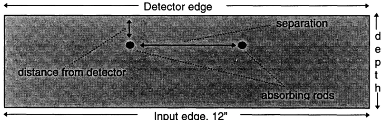
The experiments described below are all performed within a Plexiglas tank which is either one or two inches deep, twelve inches wide, and three inches high, and is filled with the Intralipid-10%TM _{solution. Each experiment}

addresses different configurations of two 'absorbers' which are also in the tank, and which distinguish themselves from experiment to experiment by being separated by different distances or by varying in their distance from the detector. Their separation is always symmetric about the center of the tank, and the two absorbers are always at equal distances from the detector. A two-dimensional picture, as if taken from above the tank, of a generic configuration is shown in Figure 2.2. 4 Detector edge

T

Figure 2.2: Arial view of a Plexiglas tank filled with Intralipid-10%TM _{solution and}

two glass rods filled with absorbing green dye.

Rods filled with absorbing green dye are inserted in four distinct experimental configurations in Jooyoun's study, and are illuminated with a .5 mW He laser light source along the edge in Figure 2.2 which is marked 'Input edge'. The output potential is measured with a photodiode amplifier along the

Measurement noise should be due mostly to quantization, and our simulation therefore includes 8-bit quantization noise, to correspond to the equipment which was used in these experiments, assuming that the gain was set to optimally detect over the varying dynamic ranges at the output [35]. This can be done with knowledge of the expected nominal output potential - the measured output potential without any added absorption.

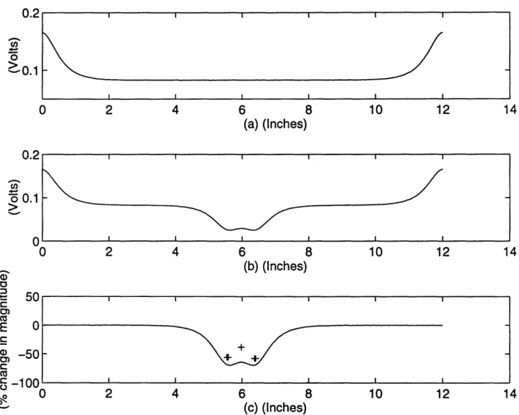
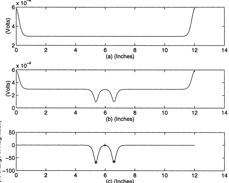
The first two experiments are performed on a tank which is one inch thick , and filled with Intralipid-10%TM solution. Figure 2.3 shows the result of a simulation of two absorbers separated by 2 cm, and which are 1.2 cm from the detector edge. The experimental result, indicated by plusses, consisted of two dips in percent change in magnitude which were approximately 2 cm apart and at fifty-six and fifty-eight percent difference.4 _{The relative peak between the dips}

was at thirty-eight percent difference in magnitude. The experimental results are closely approximated by the computer simulation, which is shown by the solid

line.

Figure 2.4 is the experimental result of two absorbers which are 3 cm apart and 2 cm from the detector edge. Experiments produced two dips which are approximately 3 cm apart. The absorbers create dips in percent differences at sixty-eight and sixty-five percent, with a relative peak between them at about zero percent difference. Again, with the same symbolic plotting conventions, the computer simulation result is very similar.

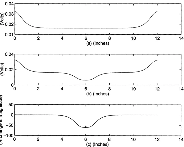
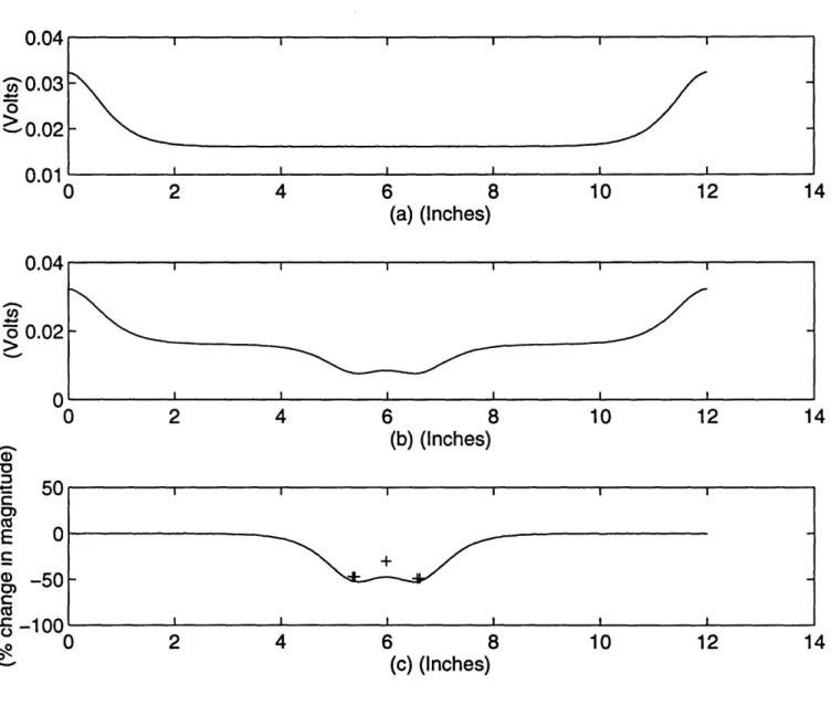
The next two experiments are performed on a slab which is two inches deep. Figure 2.5 is a measurement taken from two absorbers which are 2 cm apart and 1.5 cm from the detector edge. Experiments produced one wide dip at fifty-eight percent difference in magnitude. The simulation even duplicates this single dip! Figure 2.6 is an output measurement resulting from two absorbers which are 3 cm apart and 1.5 cm from the detector side. Experiments produced two dips at a distance of 3 cm apart, with dips in percent differences at

forty-4 The experimental results were described as having dips which had the same separation as the

absorber locations, so we assume that they coincide with the actual absorber locations, and only plot one marker representing experimental results.

4 - I I I I I 0 2 4 6 8 10 12 1 (a) (Inches) I ~ I/ 2 4 6 8 (b) (Inches) 10 12 14 14 2 4 6 8 10 12 (c) (Inches)

Figure 2.3: Two absorbers placed 2 cm apart and 1.2 cm away from the detector edge: computer simulation result (_) and experimental peak and dip locations (+); output potential due to nominal absorption (a), output potential with perturbation in absorption (b), and percent change in magnitude from the nominal to the perturbed case (c).

0.2 0 >- 0.1 0 a) '0 PA 0.2 C/) 0.1 0 .U ) C a) -50 CD' Ma -o. 0 I

I I I I I I I I I I I I 0 2 4 6 8 10 12 1 (a) (Inches) I< ' I I '- L' -LII ,- 2 4 6 8 (b) (Inches) 10 12 4 14 2 4 6 8 10 12 (c) (Inches) 14

Figure 2.4: Two absorbers placed 3 cm apart and 2.0 cm away from the detector edge: computer simulation result (_) and experimental peak and dip locations (+); output potential due to nominal absorption (a), output potential with perturbation in absorption (b), and percent change in magnitude from the nominal to the perturbed case (c).

26 0.2 0 20.1 0.2 co) 0 0.1 0 -1 a) '0 50 0) E 0 , -50 cm .c -100 o (

c,

2 4 6 (a) (Inches) 8 10 12 14 I- I I I I 0 2 4 6 8 10 12 1 (b) (Inches) I I I I I I I I I I I I It , , , , ,~~~1 12 2 4 6 (c) (Inches) 8 10 12 4 14

Figure 2.5: Two absorbers placed 2 cm apart and 1.5 cm away from the detector edge: computer simulation result (_) and experimental peak and dip locations (+); output potential due to nominal absorption (a), output potential with perturbation in absorption (b), and percent change in magnitude from the nominal to the perturbed case (c).

0 0.04 -"0.03 0 -- 0.02 0.01 0.04 0.02 o 0.02 . s~~~~~~~~~~~~~~~ a) '1 C 03 E 0) Cn 0 0a 50 0 -50 -100 ) I I I I I I I I I I I

4 0 2 4 6 8 10 12 1 (a) (Inches) I I I I I I 2 2 4 6 4 6 (b) (Inches) (c) (Inches) 8 10 8 10 12 4 4 12

Figure 2.6: Two absorbers placed 3 cm apart and 1.5 cm away from the detector edge: computer simulation result (_) and experimental peak and dip locations (+); output potential due to nominal absorption (a), output potential with perturbation in absorption (b), and percent change in magnitude from the nominal to the perturbed case (c).

28 0.04 X 0.03 0 -0.02 0.01 ( 0.04 o 0.02 0 E 0 a) -50₅₀ cu I' -100 o 1-) I I I I I I I I I I I I ) --- ·- ---·--- --- ----·- ---11 1

seven and forty-nine percent and a relative maximum peak between them at about thirty percent. Again, the simulation duplicated the experimental results well.

One problem with these simulations is that the outputs are not as strongly attenuated as we would expect, according to the number of scattering lengths which are traversed in the two depths of simulated tissue [20].

We would expect the nominal output potentials in the center of the width of the simulated tank to differ for the two different tank depths by

e(numberf space constants in one inch) Since the transport cross section for the

Intralipid-10%TM is 0.392 mm-'_{, the scattering length is about 2.5 mm, and there are about}

ten scattering lengths in an inch. Then, the difference between the two measurements should be by a factor of e ' ° _{or about 1/22,000. Instead, there is}

only a factor of five difference between the two nominal output potentials. The model does not decay exponentially with a space constant equal to the inverse of the transport cross section.

We attribute this problem to the fact that the absorption of Intralipid-1 0%TM is negligible [43, p. 2293]. We tried the same simulations with parameters which correspond to breast tissue, and this case involves an absorption coefficient which is high enough to produce nearly the expected attenuation. With these values, the transport cross section is 0.2578 mm ' _{, and the scattering length is}

about 4 mm, and so there are about 6.55 scattering lengths in an inch. The attenuation should be about e 55_{, or about 1/700. The results of this}

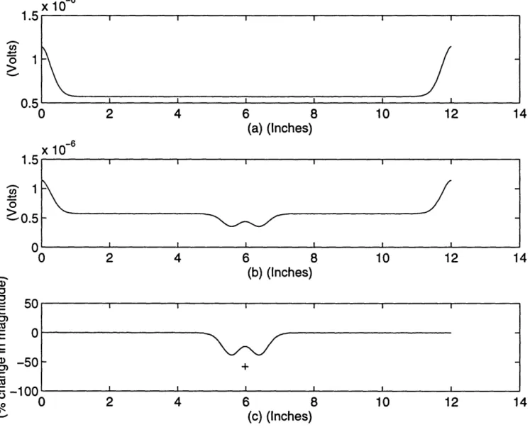
investigative simulation are shown in Figures 2.7, 2.8, 2.9, and 2.10. Their experimental configurations correspond to those of Figures 2.3, 2.4, 2.5, and 2.6, respectively. The nominal output potential in the middle of the 1" tank is

about 2.39e-4 Volts, and in the middle of the 2" tank it is about 4.23e-7 Volts. The difference between the two is a factor of 565. This is much closer to 700 than five is to 22,000. When the absorption coefficient is nearly zero (as in the

case of the simulations which model Intralipid-10%TM), the conductances to

ground are also nearly zero. We expect that this is the reason for the low 29

2 4 6 8 10 12 (a) (Inches) x 1 0 I I I I I ) 2 4 6 8 10 12 1 (b) (Inches) I I I I I I 2 4 6 8 (c) (Inches) 10 14 4 14 12

Figure 2.7: Two absorbers placed 2 cm apart and 1.2 cm away from the detector

edge: computer simulation result (_) and experimental peak and dip locations

(+); output potential due to nominal absorption (a), output potential with perturbation in absorption (b), and percent change in magnitude from the nominal to the perturbed case (c). Parameters correspond to breast tissue.

30 x 10-4 0 4 v, r) 0 6 0 >-2 0 '0_{: O} -₃ A-1 _C 50 E 0 Cr ID -50 r - -100 ( ₃ . E ... . c

6 8 (a) (Inches) 6 8 (b) (Inches) 10 10 12 14 12 14 2 4 6 8 10 12 (c) (Inches) 14

Figure 2.8: Two absorbers placed 3 cm apart and 2.0 cm away from the detector edge: computer simulation result (_) and experimental peak and dip locations (+); output potential due to nominal absorption (a), output potential with perturbation in absorption (b), and percent change in magnitude from the nominal to the perturbed case (c). Parameters correspond to breast tissue.

31 x 10- 4 I-, o4 > 0 2 4 x 10 v rn I I I I r I I I I I u 0 "0 . 2 4 03 E 0 a) -50 0r .C _{z _inn}1A (- _o 'VVn -- 0- 1-.. I r. _-4 k . -t

6 8 (a) (Inches) 6 8 (b) (Inches) 6 8 (c) (Inches)

Figure 2.9: Two absorbers placed 2 cm apart and 1.5 cm away from the detector edge: computer simulation result (_) and experimental peak and dip locations (+); output potential due to nominal absorption (a), output potential with perturbation in absorption (b), and percent change in magnitude from the nominal to the perturbed case (c). Parameters correspond to breast tissue.

32 . x10- 6 1.0 0 1 I I I I I I I - I I I I I ) 2 4 x 10-6 10 12 0.5 C 1.5 en I 0 >0.5 0 3 co> . 50 E 0 C ·) -50 0) ,- -100 1-.1 O 2 4 12 4 11 4 4 4 I I I I I I I -- -- I I I I I ) 10 10 2 12 11 I I I I I I

I

I

I

- - -

I

I

I

LI^L·_I,.. ---^l··L··-·-·l----1.1_1_·. IIC-_-__)-L··-YI-·---- I I_·l_---UI·l---1A

6 8 (a) (Inches) 6 8 (b) (Inches) 6 8 (c) (Inches)

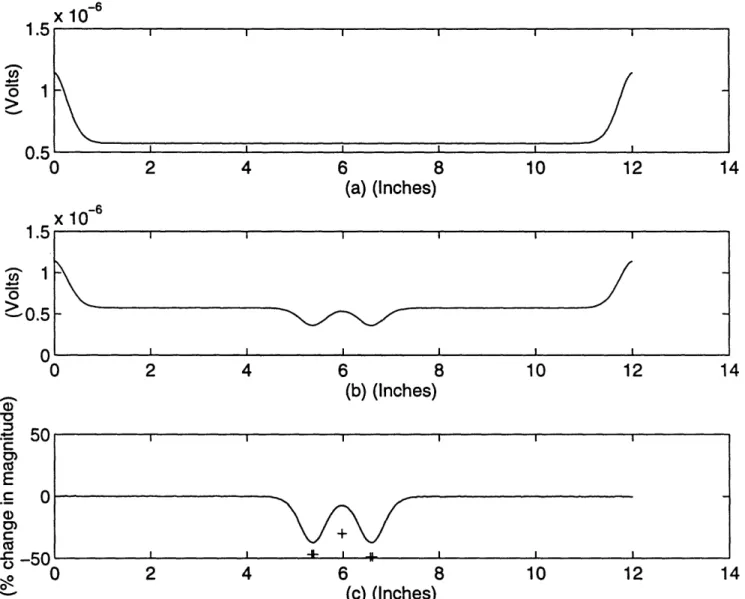
Figure 2.10: Two absorbers placed 3 cm apart and 1.5 cm away from the detector edge: computer simulation result (_) and experimental peak and dip locations (+); output potential due to nominal absorption (a), output potential with perturbation in absorption (b), and percent change in magnitude from the nominal to the perturbed case (c). Parameters correspond to breast tissue.

33 x 10-6 1. 1 I) 0 0 ) I I I I I i I I I I I I 2 4 x 10-6 10 12 14 0.5 C I . 0 a) .- 50 C 0) E .C_ 0 0) o0) C o-) 2 4 12 4 ) I I I I I I I ,I .- . I I I 10 10 2 4 4 12 1. I I I I I I

-"Z/

I

I

I - -

I

I

I

attenuation in the first set of simulations.

This series of experiments gives a good amount of initial confidence in this resistive grid model of the diffusion approximation. The experimental data was only communicated by means of peaks and dips in magnitude, so that a very precise comparison is not possible.

34

3. The Discretized Forward and Inverse Problems in Two Dimensions

First let us get a solid picture of the discrete network topology which was introduced informally in Section 2.2. The result is a simple, two-dimensional resistive grid upon which the problem can be generally defined. Recall that the model consists of a two-dimensional lattice of nodes which are connected by resistors, and each node is connected to ground through an additional resistor. A slightly more comprehensive model would extend this grid into three dimensions, and may move into the time-dependent regime.

If we let H be the number of nodes in the height of the two-dimensional grid, and let W be the number of nodes in the width of the grid, then we can implement a node-numbering sequence as depicted in Figure 3.1 below.

WHI + *|* v *+

Figure 3.1: Resistive Grid

We will refer to nodes 1 through H as the input nodes, those on the left edge of the grid, and to nodes (W-1)*H+1 through W*H as the output nodes, which are located on the right edge of the grid. The light input which is incident 35

upon the left side of the grid is modeled as current; the nodes on the right side of the grid are analogous to the light output intensities which we would measure experimentally, and in the simulation we compute the voltage potential at those locations.

3.1 General Mathematical Formulation of the Forward Problem

We consider the conductance matrix, G, to be a sum, G = Gh + G_v, the

conductance due to the horizontal resistors (those between neighboring nodes) plus the conductance due to the vertical resistors (those from each node to ground). We have a good understanding of what G is for normal, healthy tissue, and we refer to this general case as Gnom, the nominal conductance matrix. It is related to the potential, v, and the current, i, by the following equation:

Gv= i. (3.1)

In cancerous tissue, we say that there is a non-negatively-valued perturbation, G, from the nominal conductance matrix, so that we now have a conductance matrix which is equal to:

G = Gnom +6G.

We can define a forward problem which consists of determining a vector vnom of node voltages, given the conductance matrix, G nom, and the current input to

each node, i, such that:

G mvnom = i, (3.2)

or, with the perturbation, such that:

(Gnom+ SG)(Vnom+ v) = i. (3.3)

In the experimental forward problem, we are unable to measure the potential on the interior of the model. In the simulated forward problem, we may determine all of v computationally, for arbitrary geometries. Also, in the experimental forward problem, we may only inject current along the boundary; 36

-.

and specifically, only on regions of the boundary which are considered part of the input. The current everywhere else is equal to zero.

In our numbering scheme, this means that we can only measure the output potentials at the last H nodes, and that we can only inject current at the first H nodes. Since we can only measure output potentials from node [(W-1)*H+1] to node [W*H], we have only H measurements and thus H equations for each single-node current injection experiment. If we could measure all of the potential values along the grid, we would have W*H equations for each single-node current injection experiment. Since there are H injection single-nodes, we have H2 _{equations overall.}

What kind of a matrix are we dealing with here? Because G is the conductance matrix in a resistive circuit equation, it exhibits reciprocity and is therefore symmetric.5 _{Another result of its being the conductance matrix in a}

resistive circuit equation is that G is an M-matrix.6 _{As long as there is a nonzero}

conductance to ground at every node, G is strictly diagonally dominant; otherwise, it is weakly diagonally dominant. G has a sparse, Toeplitz-like

structure due to the second spatial derivative in the corresponding diffusion equation: grid neighbors which are symmetric about a node, and adjacent to it, are represented at equal distances to the right and left of an element on the main diagonal in G. The physical cause of this banded structure is the isotropic scattering.

As an example of the numerical structure of the conductance matrix, consider a single node, k, of a resistive grid, such as one of the nodes in Figure 3.1. Isotropic scattering dictates that photons propagate radially outward from their point of incidence, which we take to be grid node k. The four nearest

5 If we have any two unique electrical events on the grid and the corresponding current and

potential vectors for each, reciprocity implies that the inner product of one current vector and the other potential vector is equal to the inner product of the remaining two vectors. The network is

reciprocal since it is constructed from linear 2-terminal resistors, and reciprocity implies symmetry of the conductance matrix [22, pp. 102-103].

By definition, G then has non-positive off-diagonal entries, and its inverse is nonnegative. Because we know that it is symmetric, the fact that it is an M-matrix also implies that it is positive

definite, and all the entries in its inverse are positive [29, pp. 44, 93].

neighbors are at nodes k-1, k+1, k-H, and k+H. For each k, the node relationships between node k and these neighboring locations are represented in the conductance matrix by entries one band to the right and left of the main diagonal, and H bands to the right and left of the main diagonal. For a grid like the one in Figure 3.1 which is four nodes tall and three nodes wide, if each resistor has a resistance of 1 Ohm, then a sample conductance matrix (in mho) is: 3 -1 0 0 -1 0 0 -1 4 -1 0 0 -1 0 0 -1 4 -1 0 0 -1 0 0 -1 3 0 0 0 -1 0 0 0 4 -1 0 0 -1 0 0 -1 5 -1 0 0 -1 0 0 -1 5 0 0 0 -1 0 0 -1 O O O O -1 0 0 O O O O O -1 0 0 0 0 0 0 0 -1 O 0 0 0 0 0 0 0 0 0 0 0 0 0 0 0 0 0 0 0 0 0 -1 0 0 0 0 0 -1 0 0 0 0 0 -1 0 0 -1 0 0 -1 0 4 0 0 0 -1 0 3 -1 0 0 0 -1 4 -1 0 0 0 -1 4 -1 -1 0 0 -1 3

The matrix is nearly Toeplitz along its off-diagonals, but there are notches (zeros instead of nonzero values) at some locations in the band which is one diagonal away from the main diagonal. This results from the spatial discontinuities at the top and bottom edges of the grid, where numerically-sequential nodes (as they are indexed in Figure 3.1) are not neighbors, as a single-valued band in G would have to imply.

3.2 General Mathematical Formulation of the Nonlinear Inverse Problem

We have defined a generalized forward problem; we can similarly define an inverse problem in which we would like to find the perturbation 6G for which a

set of measured output vectors (vdom+ _(nompm ' { SVd) (the subscript 'm' represents the

nodes which we are able to measure, and the superscript 'd' represents the nodes at which we can drive with current) agree most closely with their corresponding entries in the computed set of vector expressions:

[Gnom + G;]1 i.

This expression comes from rearranging terms to isolate (v+ Sv) in Equation 3.2. The inverse problem is a nonlinear one because the matrix inverse is a

nonlinear expression in Gom + (G.

3.3 The Forward Problem Specific to this Research

This research effort focuses on the two-dimensional slice of resistive grid elements which is H nodes high and W nodes wide, as in Figure 3.1. We further simplify the problem by assuming that only the vertical conductances, those we attribute to the absorption coefficient, are perturbed in the conductance matrix

for cancerous tissue, where G = Gnom+ G.7 The elements of G are solely

along the diagonal of G, so that we may write the perturbed conductance matrix G as:

G = [Gnom+ diag(x)], (3.4)

where x is the vector of perturbations in conductance for which we would like to solve, and the 'diag' function maps a vector into a diagonal matrix. We define:

R(x) = G-'(x). (3.5)

The forward problem is then defined by solving for v due to each of the many current vectors, i, such that:

v = R(x) i. (3.6)

7 This assumption does not agree with the derivation in Chapter 1, but we will assume for now

3.4 The Nonlinear Inverse Problem Specific to this Research

In this research problem, we are more directly concerned with the inverse problem of finding G given many potential vectors, v, which are the results of many different current injections, i. To measure the agreement between the output potentials which we can measure and the corresponding potentials calculated from our guess at the perturbation in conductance, we use the squared Euclidean norm, which in this case is:

H HW 2

¢(x)= = ; A [(R(x)i)d Veas] (3-7)

d = 1 m= H(W-1)+1

The purpose of the inverse problem is to find the global minimum of this squared norm. This is difficult to do, because it is a nonlinear function. My approach at the inverse problem consists of finding a local stationary point of (x) which may or may not be its global minimum.

Note that the first term in the brackets of Equation 3.7 is actually the bottom left HxH block of the inverse of the conductance matrix. R(x) is the entire inverse of G, but the subscripts 'd' and 'm' pick out its first H columns and last H rows, respectively. Being able to inject current only at the first H nodes means that only the first H entries of i can ever be nonzero, so only the first H columns of R(x) will be preserved in the product. Also, the subscript 'm' implies that we are only considering the nodes along the output in v, so we neglect all but the last H rows of R(x)id. And thus, we are left with the bottom HxH block of R(x) in Equation 3.7.

The forward problem is known to be very insensitive since a large perturbation in absorption will result in a very small change in measured output potential. Therefore, when we observe a very small change in output potential (such as that due to measurement noise), we tend to expect that it was caused by a large perturbation in absorption. The inverse problem is therefore challenging and misleading and is referred to as being highly sensitive due to the insensitive forward problem.

The forward problem is also complicated because the G matrix, although nonsingular, is computationally prohibitive to invert due to its large size. Even if we could easily invert G, the amount of information we can learn about the

problem due to a single current injection and the corresponding set of output potentials is very low.

We approach the solution to the inverse problem by assembling a set of equations due to many injection sites and their corresponding output potentials, in an effort to compensate for both the lack of information in solving the forward problem for the result of a single current injection system and the sensitivity to measurement noise. We hope that taking many measurements will make it more clear what is noise and what is a perturbation-induced change in output

potential.

It has been suggested that increasing the number of injection sites, and therefore different i's for which we solve the forward problem, may make the inverse problem more well-determined in the continuous regime; in the discrete context of this problem, we can analogously expect an improvement in the conditioning of the problem [24, 41].8

8 A continuous partial differential equation may be characterized as 'well-determined', but in our

discrete version of the problem, this characteristic depends on the fineness of the discretization and can be measured with the condition number of the problem [41]. What happens is that each entry of the solution to a linear equation is proportional to the inverse of its corresponding

singular value [44, p. 55]. As the grid spacing becomes finer and therefore the number of

unknowns becomes very large, the number of singular values exceeds the number of independent equationsin the problem so that some of the singular values go to zero, so that thecorresponding solutions blow up [44, p. 55]. The condition number is the ratio of largest to smallest singular values, so that when the smallest singular value is near zero, the condition number will be very large and we then say that the linear operator is ill-conditioned [8, Section 2.7.2].

It should be much easier to solve the forward problem several times than to invert the conductance matrix in solving the nonlinear problem. We therefore look for ways to use the forward problem to solve the inverse problem, such as by using a modified version of Newton's Method with a quadratic cost function, a variation on a suggestion of Dr. Arridge. This topic and related issues will be discussed with references in Chapter 5.

4. Linear Formulation of the Inverse Problem

A popular approach to simplifying the nonlinear inverse problem involves linearizing about the nominal conductance, Gnom, so that a system of equations can be analyzed in terms of a perturbation of the conductance from the nominal values [24]. As stated in Section 3.3, we assume that only the vertical conductances, those along the diagonal of G, are perturbed.

We have defined vd _{as the solution to the forward problem when i is zero}

for all entries except the dth, which is equal to 1 Ampere. Similarly, em is defined as the solution to the forward problem when i is zero for all entries except the ((W-1)*H + m) ,h one of the nodes along the output, which is also equal to 1 Ampere. Given the forward problem, if we perturb G by SG such that:

(G + G)(v d+8vd) = id,

resulting in:

GVd + GV + GVd +G + GVd = id (4.1)

we can subtract the equality GVd = id from this product. We can further

subtract the nonlinear term 868vd, because the perturbation SG (and therefore

the change in output potential it induces, Svd) are small enough when compared with the other terms in the equation that their second-order product is practically negligible. These subtractions reduce the expression to:

GSVd + GVd = 0. (4.2)

How can we solve for SG ? We know all of G, the nominal conductance matrix, and all of vd, the response to the nominal G when the circuit is injected with 1 Ampere of current at node d. The fact that we can only measure the last H values of Svd suggests that we should eliminate the unknowns from the system in Equation 4.2 [20]. In the paragraphs below we do just that, and the result is a linear expression for SG which relies on the Jacobian matrix.

We first begin by separating the components of the first term in Equation

4.2 into two parts. Let Ginteror be the first (W-1)*H columns of G (corresponding

to the input nodes and interior nodes of the resistive grid model), while G eas is the last H columns of G (corresponding to the output nodes). Similarly, let

Vdnt be the first (W-1)*H entries of 8vd and let vdmeas be the last H entries. The new form of Equation 4.2 is then:

G V d + G mVd + GVd =0. (4.3) interior interior meas meas

To follow the suggestion from the paragraph above and eliminate unknowns

from Equation 4.3, we multiply the entire system by em T , which is defined at the beginning of Chapter 4. This gives:

emT (Ginterr tenor iV + Gmeas 8Veas+ SG V d) 0. (4.4)

Now, em is orthogonal to all rows of G (and therefore all of the columns,

since G is symmetric), except for the ((W-1)*H+m) a, since Gem = i m where all of

i is zero except for the ((W-1)*H+m) element.9 _{This eliminates the first term in}

Equation 4.4 due to the definition of Ginteror. This also reduces the second term

in Equation 4.4 to 1 Ampere times 6vdeas, the change in measured output

potential which is observed at node ((W-1)*H+m) due to a current injection at node d. Because SG is a diagonal matrix, with appropriate multiplying of terms, we can use its vector definition, x, from Section 3.3, and rearrange what remains of Equation 4.4 to:

(em.*Vd)T X =8 -V s, m < H and 1 < d < H. (4.5)

The '.*' represents term-by-term multiplication, so that the '.*' product of two

vectors remains a vector. Assembling this equation for all m's and all d's will result in the coefficient of x being equal to the Jacobian of the output potentials

44

9 This is due to Equation 3.1.