HAL Id: hal-01058339
https://hal.archives-ouvertes.fr/hal-01058339
Submitted on 19 Dec 2014
HAL is a multi-disciplinary open access
archive for the deposit and dissemination of
sci-entific research documents, whether they are
pub-lished or not. The documents may come from
teaching and research institutions in France or
L’archive ouverte pluridisciplinaire HAL, est
destinée au dépôt et à la diffusion de documents
scientifiques de niveau recherche, publiés ou non,
émanant des établissements d’enseignement et de
recherche français ou étrangers, des laboratoires
Dictionary of gray-level 3D patches for action
recognition
Stefen Chan Wai Tim, Michèle Rombaut, Denis Pellerin
To cite this version:
Stefen Chan Wai Tim, Michèle Rombaut, Denis Pellerin. Dictionary of gray-level 3D patches for
action recognition. MLSP 2014 - IEEE 24th International Workshop on Machine Learning for Signal
Processing, Sep 2014, Reims, France. �hal-01058339�
Dictionary of gray-level 3D patches for action
recognition
Stefen Chan Wai Tim, Michele Rombaut, Denis Pellerin
∗December 17, 2014
Abstract
This paper deals with action recognition in the context of video anal-ysis based on the use of a sparse dictionary defined by the 3D spatio-temporal representation of the actions. A 3D volume can be seen as a set of gray-level 3D patches comprising 2D patches taken in successive frames in order to capture a motion pattern. The goal of our proposal is to recognize human actions within these 3D volumes whose 3D patches are described with the dictionary atoms. To that end, we compute a mo-tion signature by building a histogram based on the use of the atoms of the dictionary. Paired with a SVM, we show that these signatures can be exploited in the context of action recognition. This method has been tested on the KTH database with good results.
1
Introduction
Action recognition research has developed a lot in the last years along with the rise of video contents, especially because its applications are numerous in surveil-lance, automatic video annotations or entertainment. Generally, it consists in extracting features either from each pixel of the whole image (or successive frames) [1], [2] or just from a few chosen pixels [3]. The goal is to classify some human activities using the data extracted from videos.
Action recognition often involves a lot of data and because of that, some techniques based on dictionaries and sparse representations [4], [5], [6] have emerged in the recent years to deal better with this aspect. These methods rely on the creation of a dictionary which can encode information contained in an image.
For the analysis of human activities, motion plays a crucial role. Usually, a motion descriptor can be computed (i.e Optical flow [7]) and the result is a 2D-based patch representation of the motion. Instead, we choose to analyse motion
∗This work has been partially supported by the LabEx PERSYVAL-Lab
directly by using the spatio-temporal volume of gray-level pixels to extend 2D spatial patches without relying on an intermediary motion descriptor.
In this paper, we propose a method relying on a dictionary of 3D atoms (2 spatial dimensions and 1 temporal dimension) which can describe local motions to classify image sequences of a few frames extracted from a video containing human activities. The remainder of the paper is organized as follows: Section 2 presents the proposed action recognition method based on a dictionary of 3D atoms. Section 3 describes the experimental results. Finally, some conclusions are presented in Section 4.
2
Method framework
In this paper, we propose a method for human action recognition in the context of 2D video sequences. We want to classify spatio-temporal volumes composed of several frames and containing a human who perfoms a particular action. We assume that these volumes are previously defined. Some examples of such volumes can be observed on Figure 4.
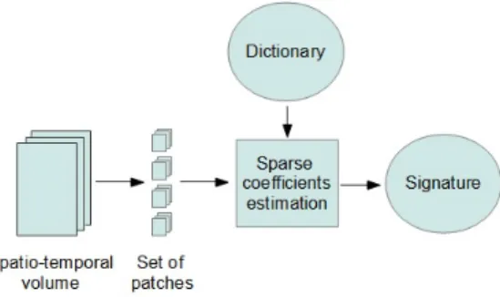
The method described below builds a 3D patch-based dictionary from spatio-temporal volumes which can represent motion. We define a 3D image patch as a succession of 2D image patches (i.e the same patch and its variations through the successive frames of a video). Hence, the dictionary can be considered as a collection of patches called atoms (see Figure 1) which can be used to describe any patches as a combination of these atoms.
The presented algorithm can be decomposed into 3 main steps : (i) Dictio-nary learning, (ii) Signature computation and (iii) Classifier training.
2.1
Dictionary learning
We have a dataset of spatio-temporal volumes at our disposal from which we can extract m 3D patches. From this set of 3D patches, we try to define the most representative dictionary. Different methods exist in the literature to learn dictionaries for sparse representation [8], [9]. We tested different dictionary learning algorithms available in the state of the art [10] and we did not notice any major difference in the results obtained by our method. Therefore, in our proposal, we decided to use the well-known K-SVD algorithm [9] to carry out the learning of the dictionary.
Starting with the notations, let p be a 3D patch of size (s × s × t), with s being the size of a square patch in the spatial dimensions and t being the number of frames considered in the temporal dimension. This patch p is reshaped and treated as a column vector of size n = s2t : p = (a
i)i∈[1,n]with aia feature (gray
level) associated to the pixel i. Each patch is normalized as : pnorm = p−¯kpkp2
where ¯p is the mean of the vector p and k p k2 is the L2-norm.
Let Y = [p1norm, p2norm, ..., pmnorm] ∈ Rn×m be a a matrix composed of 3D
Rn×Natoms be the dictionary of N
atoms atoms dk, where the number Natoms is
chosen empirically.
t = 1 t = 2 t = 3
Figure 1: Example of a 3D atom of (s × s × t) = (5 × 5 × 3) pixels from a dictionary trained with the KTH database. This atom represents a horizontal motion going from right to left.
The formulation of the dictionary learning algorithm is : min
D,X{kY − DXk 2
F} such that ∀i ∈ [1, m] , kxik0≤ T0 (1)
where X = [x1, x2, ..., xm] ∈ RNatoms×m contains the coefficients of the
decom-position of Y using the dictionary D. xi= (αj)j∈k1,Natomsk is a column vector
from X and kxik0 is the norm that counts the number of non-zero entry of the
vector. k · kF is the Frobenius norm: A ∈ Rn×m, kAkF =
q Pn
i=1
Pm
j=1|aij|2.
T0 is the maximum of non-zero entries.
K-SVD is an iterative algorithm performed in two steps on the dataset Y . In the first step, the codes X are optimized with respect to a fixed dictionary D (Sparse coding):
X(k+1)= arg min
X
{kY − D(k)Xk2
F} (2)
such that ∀i ∈ [1, m] , kxik0≤ T0.
This step can be done using the Orthogonal Matching Pursuit (OMP) [11] algorithm which is a greedy algorithm used for its efficiency.
The second step consists in the update of the dictionary D with respect to X and is done according to (Dictionary update):
D(k+1)= arg min
D
{kY − DX(k+1)k2F} (3)
The initial dictionary D(0)is initialized randomly with patches from the learning
set.
The output is an overcomplete dictionary D composed of Natoms whose
atoms can be seen as elementary motion patterns as shown in Figure 2.
2.2
Signature computation
This section explains how to compute the signature of a spatio-temporal volume containing a moving object in a video sequence. Our implementation requires
t = 1
t = 2 t = 3
Figure 2: Example of 25 atoms of size (s × s × t) = (5 × 5 × 3) pixels from a learned dictionary of KTH database. The 3 images taken together can describe elementary motion patterns.
a pre-processing step which consists in finding the localization of the humans to define the spatio-temporal volumes. This step is necessary to narrow down the region where motion occurs and can be done by using a pedestrian detector such as [12]. A spatio-temporal volume V can be decomposed into a set of overlapping 3D patches (see Figure 3). When the dictionary D is built, every patch pnormof the volume V can be described as a linear combination of atoms
dk (Equation 4). pnorm= Natoms X k=1 αk· dk ! + eerr (4)
where αk is the coefficient of atom dk and eerr is the reconstruction error.
The signature is defined as the histogram hV of the volume V characterizing
the motion inside the considered spatio-temporal volume. It is computed over this spatio-temporal volume by summing the sparse coefficients αkof each atom
of the dictionary D for all the patches of the volume.
Formally, each bin hkV associated to the atom dk of the histogram is
com-puted according to : ∀k ∈ [1, Natoms] , hkV = X pnorm∈V |αk| (5) with hV = (hkV)k∈k1,Natomsk.
Figure 3: The spatio-temporal volume is decomposed into an overlapping set of patches p which are also decomposed into a set of coefficients αk using the
learned dictionary D. These coefficients are used to build the signature which is the histogram hV.
In order to handle the use of regions of different sizes, the histogram is then normalized, such that :
Natoms
X
k=1
hkV = 1 (6)
As a consequence, a spatio-temporal volume can be represented using a his-togram. An example of the resulting histogram is displayed in Figure 4.
2.3
Classifier training
The histogram (signature) hV described in section 2.2 can model the human
motion inside the volume V which is a region of a video and can consequently be used to train a classifier in the context of action recognition using only a few frames.
For the training, signatures are computed for labeled spatio-temporal vol-umes. These signatures are then given as input to a classical multiclass SVM classifier (Figure 5). The SVM is trained using a RBF kernel.
2.4
Spatial and temporal arrangement
Since a histogram representation discards the spatial and temporal dependen-cies, decomposing the spatio-temporal volume into smaller ordered volumes can give better results [13], [14]. Moreover, we do not want to increase the number of parameters describing this spatio-temporal volume.
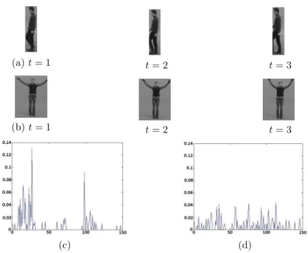
Therefore, in order to improve our representation, we divide the spatio-temporal volumes into spatio-spatio-temporal cells (Figure 6). For 3D patches, cells can be formed in both spatial and temporal dimensions. In the spatial dimen-sions, we can divide the volume into equally distributed smaller volumes which describe the motion at a specific location. In the temporal dimension, it can be done by using multiple blocks of frames: for example, we can use nt= 2 volumes
(a) t = 1 t = 2 t = 3
(b) t = 1 t = 2 t = 3
(c) (d)
Figure 4: Two examples of spatio-temporal volumes containing human actions and the corresponding histogram (signature) computed with a dictionary of Natoms= 150 trained with the KTH database: the spatio-temporal volume (a)
gives the signature (c) of a walking action and the spatio-temporal volume (b) gives the signature (d) of a handwaving action.
by computing a signature for one volume made with t frames, coupled with the signature of a second volume with t frames which results in a signature of twice the size of the original signatures. The final signature used for classification is the concatenation of the feature histograms computed for each spatio-temporal cell. Experimentally, we found that using more cells yield an improved accuracy, while the dimension of the features rises accordingly.
(a) Spatial cells (ns= 4)
(b) Temporal cells (nt= 2)
Figure 6: Examples of ”decomposition” of a spatio-temporal volume into (a) spatial and (b) temporal cells. Spatial cells are obtained by cutting the spatio-temporal volume into ns= 4 parts. Temporal cells are obtained by juxtaposing
nt= 2 consecutive spatio-temporal volumes.
3
Experimentations
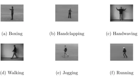
The proposed algorithm has been tested on the KTH database [15] which is a large public dataset containing videos of 25 people executing 6 types of actions (Walking, Running, Jogging, Boxing, Handwaving, Handclapping) in 4 different scenarios. These scenarios include indoor and outdoor sequences, changes in clothes and scale variations (Figure 7).
For the tests, we took 15 people divided in 2 groups, 10 for training / val-idation and 5 for testing. This is the usual ratio with this dataset [15], [16]. For each video, the spatio-temporal volumes corresponding to the human are manually annotated in a few frames, resulting in 10 computed signatures and a dataset of about 3600 samples. During the testing, classification labels are given for each sample.
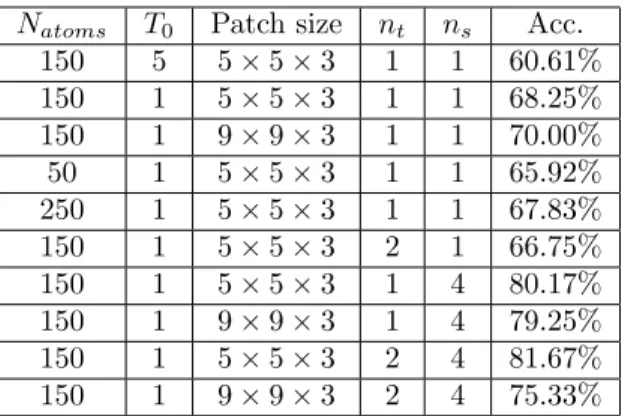
Using this dataset, we aim to perform a classification of volumes using only a few frames. Regarding the parameters of the algorithm, we took as the reference the size (s×s×t) = (5×5×3) for the 3D patches, Natoms= 150 for the dictionary
size and T0= 1 to define the number of atoms used to decompose one patch.
The dictionary is learned using the patches extracted from the spatio-temporal volumes of one person from the dataset for all actions and all scenarios. The SVM classifier is trained using a cross-validation paired with a gridsearch for the parameters. The results presented below are the results of the classification for the motion signature of each spatio-temporal volume taken independantly: no label is given to the videoclips.
The parameters that can be changed in the method are the patch size (s × s × t), the number of atoms in the dictionary Natoms, the number of non-zero
entry T0used for the decomposition of 3D patches and the number of temporal
and spatial cells, ntand ns respectively, to take into account sequentiality and
(a) Boxing (b) Handclapping (c) Handwaving
(d) Walking (e) Jogging (f) Running
Figure 7: Example of the actions performed within the KTH Dataset : ”Box-ing”, ”Handclapp”Box-ing”, ”Handwav”Box-ing”, ”Walk”Box-ing”, ”Jogging” and ”Running”. Each action is executed in different conditions: indoor and outdoor, with clothes and scale variations.
assess the limits of the proposed signature. The results for some of the setups are given in Table 3.
First, for the choice of T0 we found that T0 = 1 gives out slightly better
results than T0 = 5 or T0 = 7. Moreover, the number of atoms contained in
the dictionary and the choice of the patch size also have an influence on the results. We tested different patch sizes: t = 3 and t = 2 for the size in the temporal dimension. The results are slightly better for t = 3. Another reason is to emphasize the spatio-temporal volume aspect. For the spatial dimensions, s = 9 and s = 5 lead to similar results. We evaluated 3 dictionary sizes: Natoms= 50, Natoms= 150 and Natoms= 250. The classification performances
decrease a little for the smaller dictionary and do not vary much between the two others. We found that Natoms = 150 is a good choice for this dataset because
the dimension of the signature increases rapidly when we use the division into cells.
We remind that the final signature is the concatenation of the signatures of the different cells (section 2.2). In the configuration, the spatio-temporal volume is divided into ns = 4 regions in the spatial domain and into nt = 2
regions into the temporal domain resulting in 8 spatio-temporal cells in totals. As a consequence, the final signature size is 1200. The choice of using temporal and spatial cells greatly improved our result from 68.25% to 81.67%.
The confusion matrix given in Table 3 shows the repartition of classification errors for the best configuration.
In [16], some classification results are given for the same dataset using various spatio-temporal features. We are in totally different conditions in our
experi-Natoms T0 Patch size nt ns Acc. 150 5 5 × 5 × 3 1 1 60.61% 150 1 5 × 5 × 3 1 1 68.25% 150 1 9 × 9 × 3 1 1 70.00% 50 1 5 × 5 × 3 1 1 65.92% 250 1 5 × 5 × 3 1 1 67.83% 150 1 5 × 5 × 3 2 1 66.75% 150 1 5 × 5 × 3 1 4 80.17% 150 1 9 × 9 × 3 1 4 79.25% 150 1 5 × 5 × 3 2 4 81.67% 150 1 9 × 9 × 3 2 4 75.33%
Table 1: Table containing the results of accuracy with different configurations of the dictionary or the feature. As we can see, adding nt = 2 temporal and
ns= 4 spatial cells increases the classification accuracy since it gives back some
spatial localization information which is lost when building a histogram.
W alk Box W ave Clap J og Run W alk 0.92 0 0 0 0.10 0.01 Box 0.01 0.84 0.04 0 0 0 W ave 0.02 0.15 0.77 0.05 0 0 Clap 0 0.05 0.19 0.95 0 0 J og 0.05 0 0 0 0.75 0.30 Run 0 0 0 0 0.15 0.69
Table 2: Confusion matrix for a dictionary learned on (5 × 5 × 3) patches, with 150 atoms and 8 spatio-temporal cells. Average accuracy for spatio-temporal volume classification is : 81.67%.
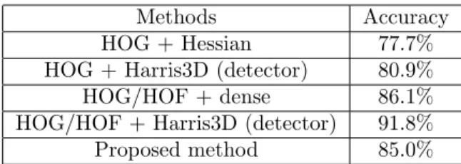
ment since we only evaluated a subset of the KTH database and only a small part of each video. However, in order to propose a comparison with these meth-ods, we used the results of the volume classification as votes to label the videos. The class label assigned to a video corresponds to the class which contains most its volumes. In order to decide between 2 classes with equal number of votes, the longest succession of volumes assigned to the same class is taken into ac-count. Table 3 shows the results obtained. As we can see the accuracy in this configuration increases: 85% instead of 81.67%. This result is due to the fact that even if we have some false classifications within a given video, the majority of frames are well classified resulting in a valid classification for the whole video.
Methods Accuracy HOG + Hessian 77.7% HOG + Harris3D (detector) 80.9% HOG/HOF + dense 86.1% HOG/HOF + Harris3D (detector) 91.8% Proposed method 85.0%
Table 3: Performance comparison for different features for the classification of videoclips. The results for the other features are obtained in [16] using histogram representations and Bag of Words model with a codebook size of 4000. For the proposed method, video labels were given by using the label given to the volumes as votes.
4
Conclusion
We have presented in this paper a new dictionary of 3D patches used to describe human motions. This new system can decompose spatio-temporal volumes into a motion signature that can be applied in the context of action recognition. One advantage of this method is that the classification of an action can be performed using only a reduced number of frames. This method has been tested on the KTH database with good results. Please note that the parameter choices presented in this paper depend on the database.
For future work, we are looking for dictionary reduction methods, to in-crease the dictionary effectiveness and build more complex signatures without increasing drastically their dimensions.
References
[1] A. A. Efros, A. C. Berg, G. Mori, and J. Malik, “Recognizing action at a distance,” ICCV, 2003.
[2] K. Schindler and L. V. Gool, “Action snippets: How many frames does human action recognition require?,” CVPR, 2008.
[3] P. Scovanner, S. Ali, and M. Shah, “A 3-dimensional sift descriptor and its application to action recognition,” Proceedings of the 15th international conference on Multimedia, 2007.
[4] J. Yang, K. Yu, Y. Gong, and T. Huang, “Linear spatial pyramid matching using sparse coding for image classification,” CVPR, 2009.
[5] T. Guha and R. K. Ward, “Learning sparse representations for human action recognition,” IEEE Transactions on Pattern Analysis and Machine Intelligence, vol. 34, 2012.
[6] G. Somasundaram, A. Cherian, V. Morellas, and N. Papanikolopoulos, “Action recognition using global spatio-temporal features derived from sparse representations,” CVIU, 2013.
[7] K. Jia, X. Wang, and X. Tang, “Optical flow estimation using learned sparse model,” ICCV, 2011.
[8] T. Dean, G. Corrado, and R. Washington, “Recursive sparse, spatiotem-poral coding,” Proceedings of the Fifth IEEE International Workshop on Multimedia Information Processing and Retrieval, 2009.
[9] M. Aharon, M. Elad, and A. Bruckstein, “K-svd: an algorithm for designing overcomplete dictionaries for sparse representation,” IEEE Transactions on Signal Processing, vol. 54, 2006.
[10] F. Bach, R. Jenatton, J. Mairal, and G. Obozinski, “Optimization with sparsity-inducing penalties,” Foundations and Trends in Machine Learning, vol. 4, pp. 1–106.
[11] R. Rubinstein, M. Zibulevsky, and M. Elad, “Effcient implementation of the k-svd algorithm using batch orthogonal matching pursuit,” CS Technion, 2008.
[12] P. F. Felzenszwalb, R. B. Girshick, D. McAllester, and D. Ramanan, “Ob-ject detection with discriminatively trained part based models,” PAMI, 2010.
[13] I. Laptev, M. Marszalek, C. Schmid, and B. Rozenfeld, “Learning realistic human actions from movies,” CVPR, 2008.
[14] M. Marszalek, C. Schmid, H. Harzallah, and J. van de Weijer, “Learning object representations for visual object class recognition,” The PASCAL VOC07 Challenge Workshop, in conjonction with ICCV, 2007.
[15] C. Schuldt, I. Laptev, and B. Caputo, “Recognizing human actions: A local svm approach,” ICPR, 2004.
[16] H. Wang, M. M. Ullah, A. Klaser, I. Laptev, and C. Schmid, “Evaluation of local spatio-temporal features for action recognition,” British Machine Vision Conference, 2009.