HAL Id: inria-00171083
https://hal.inria.fr/inria-00171083v4
Submitted on 29 Jan 2008
HAL is a multi-disciplinary open access
archive for the deposit and dissemination of
sci-L’archive ouverte pluridisciplinaire HAL, est
destinée au dépôt et à la diffusion de documents
process number
David Coudert, Jean-Sébastien Sereni
To cite this version:
David Coudert, Jean-Sébastien Sereni. Characterization of graphs and digraphs with small process
number. [Research Report] RR-6285, INRIA. 2008, pp.26. �inria-00171083v4�
a p p o r t
d e r e c h e r c h e
ISRN
INRIA/RR--6285--FR+ENG
Thème COM
Characterization of graphs and digraphs with small
process number
David Coudert — Jean-Sébastien Sereni
N° 6285 — version 2
David Coudert
∗, Jean-S´
ebastien Sereni
†Th`eme COM — Syst`emes communicants Projets Mascotte
Rapport de recherche n° 6285 — version 2 — version initiale Septembre 2007 — version r´evis´ee Janvier 2008 — 26 pages
Abstract: The process number of a digraph has been introduced as a tool to study rerouting issues in wdm networks. We consider the recognition and the characterization of (di)graphs with process number at most two.
Key-words: Rerouting, process number, vertex separation, pathwidth.
This work was partially funded by the anr jc Osera, and by European projects ist fet Aeolus and COST 293 Graal.
∗MASCOTTE, INRIA – I3S(CNRS/UNSA), Sophia Antipolis, France. [email protected] †Institute for Theoretical Computer Science (iti) and Department of Applied Mathematics (kam) Charles
process number
R´esum´e : Le process number d’un graphe orient´e a ´et´e introduit pour ´etudier des probl`emes de reroutage dans les r´eseaux wdm. Nous nous int´eressons ici `a la reconnaissance et `a la caract´erisation des graphes et graphes orient´es ayant un process number au plus 2.
In a Wavelength Division Multiplexing (wdm) network, each connection request — called lightpath in this context — is assigned a route in the network and a wavelength, under the constraint that two lightpaths sharing a link must have different wavelengths.
Usually, when connection requests are added or removed from a wdm network, the routing of older connections is not modified. Hence, it is likely that after some additions and removals the overall use of resources is far from optimal. So a new request may be rejected even if it could be added up to a whole rerouting of older requests. This is the case in the example of Fig. 1, where the wdm network consists of a path of order 6 with two wavelengths λ1 and λ2. Initially (Fig. 1(a)), request (1,6) is routed on λ1, and requests
(1,3) and (5,6) are routed on λ2. Then request (1,6) is removed and a new request, (1,4),
is routed on λ1. Note that this is the only possibility to route this request without doing
any rerouting (Fig. 1(b)). In the depicted situation, a new request (3,6) has to be rejected, although the routing of Fig. 1(c) would allow to satisfy all requests. Thus, operators have to reorganize regularly the routing of all requests so as to make better use of the resources. However, they usually want to also ensure a continuous service, i.e. once a request has been accepted and routed, it is not possible to stop its routing, even for a short time. So the service offered by the operator is never lost. We are interested in the problem of going from a routing to another without loss of services.
2 3 4 5 6
1
1 2
(a) Initial routing of (1,6), (1,3) and (5,6)
2 3 4 5 6
1
1 2
(b) Removal of (1,6) and addi-tion of (1,4) 2 3 4 5 6 1 1 2 (c) Solution with (1,3), (1,4), (3,6) and (5,6)
Figure 1: Starting from the routing of Fig. 1(a), the removal of request (1,6) and addition of request (1,4) gives the routing of Fig. 1(b). Request (3,6) can not be added in Fig. 1(b), although the routing of Fig. 1(c) is possible.
Given a wdm network, a set of connection requests I and two different routings for it in the network, R1 and R2, we want to switch from routing R1 to routing R2. For every
request u, we let Ri(u) be its routing in Ri, for i ∈ {1, 2}. Consider two requests u and
v. If R2(u) ∩ R1(v) 6= ∅, i.e. the routing of request u in R2 uses resources already used
by the routing of request v in R1, then the request v has to be rerouted before we can
reroute request u. A request might be switched to an intermediate route, that uses available resources. For instance, the operator may reserve a dedicated wavelength in the network for temporary routes. We assume that each request cannot be switched to more than one temporary route, that is the next routing of a request routed on a temporary route has to be
its final routing. When a request that was previously switched to a temporary route reaches its final routing, then the freed resources can be used again, for another request. While independent switching of requests can be made simultaneously, we consider, for matter of exposition, that only one request is switched per unit of time.
We model the problem as follows: we construct a directed graph D = (V, A), where each vertex u corresponds to one request, and there is an arc from vertex u to vertex v if and only if R2(u) ∩ R1(v) 6= ∅. A vertex is said to be processed as soon as its corresponding request
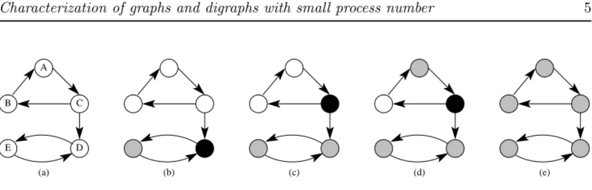
has been rerouted. We introduce the notion of Temporary Memory Unit (tmu): routing the request u on an intermediate route corresponds to putting the vertex u in a tmu. Therefore, a vertex can be processed if and only if all its outneighbors are either processed or in tmu. Note that a vertex without any outneighbor can be processed at any time. There are two basic operations: process a vertex according to the preceding rule; put a vertex in tmu. Fig. 2 shows the processing steps of a graph using one tmu.
Observe that once placed in a tmu, a vertex cannot recover its original state: it has to be processed. Nevertheless, it can occupy its tmu as long as desired. Processing a vertex which occupies a tmu frees the tmu, so that it can immediately be used by another vertex. The digraph is said to be processed when all its vertices have been processed. The problem is hence to find a suitable order to process all the vertices. If we do not want to use any tmu, then such a vertex ordering exists if and only if the digraph is acyclic; and in this case a processing order can be found in linear time. On the contrary, if we can use an arbitrary large number of tmus, then we can first put all vertices in tmu and then process them in any order. We aim at minimizing the number of tmus simultaneously in use. The process number p(D) of a digraph D is the minimum number of tmus for which there exits a process strategy for D. Notice that the process number is upper bounded by the minimum forward vertex set number, that is the smallest number of vertices which intersect all directed cycles. A process strategy that uses p (at most p, at least p, respectively) tmus is called a p-process strategy ((≤ p)-process strategy, (≥ p)-process strategy, respectively).
Observe that adding loops to a digraph D increases the process number by at most one, and it is straightforward to construct a loopless digraph D0 such that p(D) = p(D0). Hence, unless stated, we consider in the sequel loopless digraphs. When D is symmetric, we work for convenience on the underlying undirected graph G = (V, E).
An important invariant for digraphs and graphs is the notion of vertex separation. Let D = (V, A) be a digraph and X a subset of its vertices. The outneighborhood of X in D is
N+(X) := {v ∈ V \ X : there exists u ∈ X such that (u, v) ∈ A}.
A layout L of D is an ordering of the vertices, i.e. a one-to-one correspondence between V and {1, 2, . . . , |V |}. The vertex separation of (D, L) is the maximum, over all indices i ∈ {1, 2, . . . , |V |}, of the size of the outneighborhood of {L−1(1), L−1(2), . . . , L−1(i)}. The vertex separation vs(D) of D is the minimum, over all orderings L, of the vertex separation of (D, L). Note that this notion naturally extends to undirected graphs. In this case, Kin-nersley [9] proved that the vertex separation of any undirected graph equals its pathwidth. The pathwidth is an important invariant of graphs which was introduced by Robertson and Seymour [11].
B C
D E
(a) (b) (c) (d) (e)
Figure 2: Processing of a graph: processed vertices are in grey and vertices in tmu are in black. In (a), every vertex has at least one outneighbor in the initial state, so we must put a vertex in tmu. In (b), the vertex D has been put in tmu, which allows to process the vertex E. To reach the state (c), put C in tmu, which allows to process D since all its outneighbors are either processed or in tmu.
The following result establishes a close link between the vertex separation and the process number of a digraph. It was first proved by Coudert et al. [4], but we recall the proof here for completeness.
Proposition 1. For every digraph D, vs(D) ≤ p(D) ≤ vs(D) + 1.
Proof. Consider a p-process strategy for D, and let L be the order in which the vertices are processed. Observe that if the strategy is stopped just after the ith vertex has been
processed, then any non-processed vertex having a processed inneighbor must be in tmu. As this is true for every i ∈ {1, 2, . . . , |V | − 1}, this exactly means that the vertex separation of (D, L) is p, so vs(D) ≤ p(D).
Let L be an ordering of the vertices of D, and let vs be the vertex separation of (D, L). We consider the process strategy for D that consists of processing the vertices in the increasing order induced by L. At any time, let P be the set of processed vertices and let M be the set of vertices in tmu. At each step, we ensure that M := ND+(P ).
The first vertex can be processed by putting its at most vs neighbors in tmu. Suppose that i ≥ 1 vertices have been processed, and let v be the next vertex to be processed. If v /∈ M , then as the vertex separation of (D, L) is vs we infer that |M ∪ (N+(v) \ P )| ≤ vs,
so we can put all the outneighbors of v that are not in M ∪ P in tmu and process v. This uses at most vs tmus simultaneously. If v ∈ M , then |M \ {v} ∪ (N+(v) \ P )| ≤ vs, so
putting all the outneighbors of v not in M ∪ P in tmu uses at most, and possibly, vs +1 tmus simultaneously. Hence, p(D) ≤ vs +1.
As determining the vertex separation of an arbitrary graph is APX [6], the preceding result shows that the process number problem also is.
The next proposition characterizes the optimal process-strategies for digraphs whose process number is different from their vertex separation.
Proposition 2. For any digraph D, there exists a p(D)-strategy such that each vertex is in tmu before being processed if and only if p(D) = vs(D) + 1.
Proof. Suppose that the digraph D has a p(D)-process strategy such that each vertex is put in tmu before being processed. Let v1, v2, . . . , vn be an enumeration of the vertices
of D in the order in which they are processed. For each i ∈ {1, 2, . . . , n}, we set Xi :=
{v1, v2, . . . , vi}. Stop the strategy just before the vertex viis processed. All the outneighbors
of the vertices of Ximust be in tmu, and so is also vi. Therefore, |N+(Xi)| ≤ p(D) − 1 for
each i ∈ {1, 2, . . . , n}, and hence vs(D) ≤ p(D) − 1. So vs(D) = p(D) − 1 by Proposition 1. Conversely, suppose that p(D) = vs(D) + 1. Let H be the digraph obtained from D by adding a loop to each vertex that does not have one already. Thus, any strategy that processes H must put each vertex in tmu before processing it. Moreover, vs(H) = vs(D) and p(D) ≤ p(H). Since p(H) ≤ vs(H) + 1 by Proposition 1, we infer that p(H) = p(D). Therefore, any p(D)-strategy for H is a p(D)-strategy for D that put each vertex in tmu before processing it, as wanted.
The pathwidth of a graph is also its node-search number, and is closely related to other graph-searching invariants [1, 15]. Further study of the links between the process number, the vertex separation and also the search number has been performed recently [4, 14]. We refer the reader to the recent survey of Fomin and Thilikos about graph-searching [7].
We focus on the problem of recognition and characterization of digraphs and graphs with small process numbers. In Section 2, we first identify graphs whose connectivity equals their process number (Theorem 3). Then, we characterize graphs with process number at most two in terms of excluded minors and we also provide a structural description (Theorem 6). We moreover show how such graphs can be recognized and processed in linear time (Subsec-tion 2.2). We turn to digraphs in Sec(Subsec-tion ??. We characterize digraphs with process number at most two (Lemma 14), and show how to recognize whether a graph D has process number at most two (and if yes how to process it) in time O(n2(n + m)), where n is the number of
vertices of D, and m its number of arcs (Proposition 17).
2
Graphs
We start by characterizing the graphs whose connectivity is equal to their process number. Theorem 3. A p-connected graph G can be p-processed if and only if there exists a neigh-borhood of size p whose deletion induces an independent set in G.
Proof. Let G be a p-connected graph. If there is a set of p vertices of G whose deletion induces an independent set, then G has process number at most p (and hence exactly p since the minimum degree of G is at least p).
Conversely, let G be a p-connected graph with p(G) = p and consider a p-strategy for G. Stop the strategy just before processing the first vertex v. By the p-connectivity, G has minimum degree p, so v has degree exactly p, and all its neighbors are in tmu. Let A be
(a) K4 (b) H0 (c) H1 (d) H2 (e) C5
Figure 3: Some minor-obstructions for 2-processed graphs.
the set of vertices whose neighborhood is included in N (v) — and hence is exactly N (v), by the p-connectivity. Without loss of generality, we can assume that the first steps of the strategy are to process all vertices of A. If all the vertices not in N (v) have been processed, then the set N (v) fulfills the desired condition.
Otherwise, there exists a vertex w /∈ A ∪ N (v). Define z to be the next vertex to be processed. Since the strategy uses p tmus and all the vertices of A have already been processed, z ∈ N (v). Moreover, N (z) ⊂ N (v) ∪ A. Thus, N (A ∪ {z}) ⊆ A ∪ N (v). Consequently, N (v) \ {z} is a set of p − 1 vertices whose deletion disconnects w from A ∪ {z}, a contradiction.
The class of graphs with process number at most p is closed under minors. Indeed, assume that there exists a p-strategy for a given graph G. Let G0 be the minor of G obtained by contracting the edge uv into a single vertex w. Without loss of generality, suppose that u is processed before v — hence v is in a tmu when u is processed. Apply the strategy to G0. The first step concerning the vertices u, v is to put one of them in tmu. Instead, put w in a tmu. The remaining of the strategy can then be applied, ignoring the processing of u, and processing w instead of v. Thus, G0 also has process number at most p.
We focus on graphs with small process number. The first interesting case is when p is two, since only independent sets can be 0-processed and only the stars have process number exactly one. We note here that Bodlaender proved that every minor-closed class of graphs that does not contain all planar graphs has a linear time recognition algorithm [2]. This result follows from a linear time algorithm that determines whether a graph has treewidth, or pathwidth, at most k, and if so finds a tree decomposition, or a path decomposition, of width at most k, respectively. However, this algorithm is rather impracticable [12].
2.1
Graphs with process number two
In this section, we characterize graphs with process number at most two.
Lemma 4. Let K be one of the graphs of Fig. 3. Every graph with a K-minor has process number at least three.
Lemma 5. Let K consist of three subgraphs chosen among Ta, Tb and Tc and merged at
(a) Ta (b) Tb (c) Tc
(d) T1 (e) T2
Figure 4: T1 and T2 are two of the 10 non-isomorphic minor-obstructions for 2-processed
graphs obtained using 3 subgraphs chosen among Ta, Tb and Tc and merged at vertex .
Given a subgraph or a set of vertices X of a graph G, a subgraph H of G − X is attached to a vertex x of X if x is the only vertex of X adjacent to a vertex of H in G. We can now give a complete characterization of graphs that can be 2-processed. Let M1be the collection
of graphs depicted in Fig. 3 and let M2 be the collection of graphs defined in Fig. 4.
Theorem 6. For every connected graph G = (V, E), the following assertions are equivalent. (a) p(G) ≤ 2;
(b) G does not contain any of the graphs of M1∪ M2 as a minor;
(c) G consists of vertices a1, a2, . . . ar, r ≥ 1, such that each consecutive pair ai, ai+1 is
joined by an arbitrary number (at least one) of edges {ai, ai+1} or paths
n
ai, bji, ai+1
o , j ∈ N, along with an arbitrary number of subgraphs Gli attached to ai, l ∈ N, where
each graph Gli is a star.
Proof. The fact that (a) implies (b) follows from Lemmas 4 and 5. Let us show now that (b) implies (c).
We prove the assertion by induction on the number of vertices of G, the result being true if G has at most 3 vertices.
Suppose first that G is 2-connected. Thus, it has a cycle C of length 3 or 4, because G has no C5-minor. If G has a 3-cycle C, then there exists a vertex d adjacent to at least 2
vertices of C, and exactly 2 since G has no K4-minor. Let a and b be those two vertices,
and let c be the third vertex of C. Since G contains no H1, the vertices c and d have degree
2 in G. Therefore, G consists of the edge ab and some vertices of degree 2 adjacent to a and b, and hence G fulfills condition (c). Assume now that G has no 3-cycle, hence G has an induced 4-cycle C. If G is a 4-cycle, then the conclusion follows, so let assume that v is a vertex of G not in C. We can moreover assume that v has at least 2-neighbors in C. Since G has no C5, the vertex v has exactly 2 neighbors in C, which are not adjacent. The
vertices a and c, and hence G satisfies condition (c).
We assume now that G has a cut-vertex v. Let Z1, Z2, . . . Zn be the connected
compo-nents of G − v, and for each index i let Di:= Zi+ v. If each Zi is a star, then setting r := 1
and a1:= v shows that G satisfies (c). So we assume that Z1is not a star. We note that at
most two components Zi may not be stars since G has no graph of M1∪ M2as a minor.
We assume first that only Z1 is not a star. By the induction hypothesis, D1 fulfills
condition (c), so we let A0:= {a01, a02, . . . , a0s} and B0 be as stated in condition (c). Observe
that we can moreover assume that each vertex a0
iwith 1 < i < s is a cut-vertex of D1, such
that exactly two components of D1− ai are not stars. In particular, for i ∈ {1, s} the vertex
a0ihas a neighbor not in A0∪ B0. Moreover, we may assume that no vertex a0iwith 1 < i < s has degree 2, for otherwise we can consider them as vertices of B0. If v ∈ A0 then the graph G fulfills condition (c), the components Z2, . . . , Zn being just additional stars attached to
v. If v ∈ B0, say v = b1
i for some index i, then a0i or a0i+1 has degree 2 in G for otherwise
G would contain a H1 or H2 as a minor. By symmetry, we assume that a0i+1 has degree 2,
hence i = s − 1. Setting A := A0\ {a0
s} ∪ {v} and B := B0\ {v} ∪ {a0s} shows that G fulfills
condition (c). Finally, assume that v belongs to a star S := G1
i. If v cannot be considered
as the center of S, then by our assumption on A0 and because G has no minor from M2, we
infer that i ∈ {1, s}, say i = 1. Moreover, note that va1 is not an edge of G, for otherwise
G would contain H2. Let w be the center of S. Setting A := A0∪ {w, v} yields the desired
conclusion. If v is the center of S, then a similar argument (with w = v) applies if i ∈ {1, s}. So, suppose that 1 < i < s. Then the subgraph induced by ∪j>2Diis a star since G has no
minor from M2. Thus G has the desired structure.
It remains to deal with the case where another component Zi, say Z2, is not a star. Let
A00:= {a00
1, . . . , a00t} and B00be as given by condition (c) applied to the graph D2. We make
the same assumption on A00 as on A0, i.e. every vertex a00i with 1 < i < t is a cut-vertex of D2 and exactly two components of D2− ai are not stars. We also assume that such a
vertex a00i has degree more than 2. If v ∈ A0 then v = a0i with i ∈ {1, s} by condition (b). Similarly, if v ∈ A00 then v = a00j with j ∈ {1, t}. In this case, setting A := A0∪ A00 yields
the desired conclusion. So suppose that v /∈ A0. Let a0
i be a vertex of A0 closest to v. We
infer that i ∈ {1, s} by condition (b), say i = 1. Note that v cannot then belong to B0. So v belongs to a star Gl
1, and let w be the center of this star — if possible w = v. Similarly,
either v ∈ A00 or v belongs to a star attached to a001 or a00t. In the latter case, let u be the center of this star, letting u be w if possible. Setting A := A0∪ {w, v, u} ∪ A00shows that G
fulfills condition (c). In the former case, we set A := A0∪ {w, v}. This concludes the proof of the assertion.
It remains to show that (c) implies (a). The graph G can be 2-processed as follows. (1) Put a1 in tmu and set i := 1, (2) while i < r, process all subgraphs Gli (this uses a second
tmu, which is freed at the end), (3) put ai+1 in tmu, (4) process all vertices bji, (5) process
the vertex ai (which frees a tmu) and increment i.
Figure 5: A typical graph with process number two.
Corollary 7. Given two graphs H and H0 that can be 2-processed and their corresponding paths a1, a2, . . . , ar for H and a01, a02, . . . , a0s for H0, the graph G built from the union of H
and H0 and where vertices ar and a01 are merged can be 2-processed.
Proof. By the construction, G satisfies condition (c) of Theorem 6.
2.2
An algorithm to recognize graphs with process number at most
two
We present a linear time and space complexity algorithm for deciding whether a graph can be 2-processed. The idea of the algorithm is as follows. First, we note that we can decide whether a graph is a star in time O(|N (u)| + |N (v)|), where u is any vertex of that graph and v ∈ N (u), since one of them must be the center of the star. Then, if we are given the vertex a1 of condition (c) of Theorem 6, we can process all attached stars in time linear in
their size, then identify the vertex a2, and so process the graph. Also, starting from vertex
aiand thanks to Corollary 7, we can identify in linear time the vertex a1. Thus, the core of
the algorithm is, starting from any vertex u, to identify in linear time a vertex ai, which is
done using a proper analysis of the size of the neighborhoods at distance one and two of u. Before going into details, we need some more ground work. We show that deciding whether a graph can be 2-processed can be done in linear time. To this end, we first note in Proposition 8 that we can decide very efficiently if a graph can be 1-processed, and in Proposition 9 that we can decide in linear time if a 2-connected graph can be 2-processed.
From now on, we assume that a vertex u of G contains the list N (u) of its neighbors, its degree, a Boolean variable u.active set tofalseif the vertex is in tmu or if it has been
processed, and an integer — or a pointer — u.tag, which is set to a if the vertex u is visited
while processing vertex a. We also assume that we can access any vertex of G in constant time, and finally that χ(u, v) is a function which returns in constant time 1 if v ∈ N (u) and 0 otherwise. More precisely, the function χ uses an array of size |V (G)| initialized to 0. Neighbors of a are set to 1 at the beginning of the processing phase and set back to 0 at the end of the processing phase which can thus be done in time O(|N (a)|). So, the overall cost due to the management of χ for all vertices of type ai (see Theorem 6) is linear in the
if G can be 1-processed or not, where v is any neighbor of u.
Proof. Since a star has at most one vertex of degree more than one, it is sufficient to check that:
if |N(u)| > 1, then every neighbor of u has degree one. This can be checked in time O (|N (u)|);
if |N(u)| = 1, then the unique neighbor v of u cannot have neighbors of degree larger than one, which can be checked in time O (|N (v)|).
So, overall, the time complexity is O (|N (u)| + |N (v)|).
Proposition 9. Given a 2-connected graph G, we can decide in linear time if G can be 2-processed.
Proof. Let n ≥ 3 be the order of G. According to Theorem 3, we know that G should be either K2,n−2 or K2,n−2 plus an edge joining the two vertices of the bipartition of size
two. This can be verified as follows: we choose three arbitrary vertices of G. One of them must have degree two and we call a and b its neighbors. Now it remains to check that the neighborhood of each vertex v ∈ V \ {a, b} is exactly {a, b}. This procedure is linear in time.
Proposition 10. Given a graph G, we can check in linear time if p(G) ≤ 2. Proof. The proof consists of three steps.
(1) First, we prove that if we are given a graph G and a vertex a, then we can decide in linear time if G can be 2-processed under the constraint that a is the vertex a1of condition (c)
of Theorem 6. To this end, let us analyze the algorithm described in the proof of Theorem 6. We set a1:= a, and we suppose that we are at step i ≥ 1 of the loop.
Put the vertex ai in tmu: We just have to set the Boolean variable ai.activetofalse.
Remove from G all subgraphs of kind Gl
i: First, we have to determine which neighbors
of ai belong to stars and which are of type aior b j
i. According to Proposition 8 we can
decide whether a neighbor u of aibelongs to a star or not in time O (|N (u)| + |N (v)|),
where v is a neighbor of u, if any. Note that we consider the degree of u and v minus χ(ai, u) and χ(ai, v), respectively. Simultaneously, we place a tag on all neighbors
of u and v, to avoid double checking. If u belongs to a star, we process it in time O (|N (u)| + |N (v)|), that is setting the Boolean variablesactiveto false. So edges of
stars will be visited twice during the processing of vertex ai. We also visit all edges
Determine the vertex ai+1 and process all vertices bji: To determine the next vertex
ai+1, we have to check that all remaining neighbors of degree one (vertices of type bji,
if any) have the same neighbor, which should also be the remaining neighbor of degree more than 1. (Note that there is such a neighbor for otherwise the previous step would have processed all the neighbors of a.) Then it remains to process vertices of type bji. During this step, we visit all remaining neighbors of ai once.
A graph G satisfies condition (c) of Theorem 6 with the vertex a being the vertex a1 if
and only if this algorithm processes the whole graph. Note that the algorithm fails if more than one vertex are candidate to be the vertex ai+1.
Overall, each edge of G is visited twice and a constant number of operations are performed for each vertex. So we can process G in linear time.
(2) According to the previous step and Corollary 7, given a graph G and a vertex ai, we
can check in linear time if G can be 2-processed or not. Indeed, we process all subgraphs of G attached to ai that can be 1-processed. Now G − ai must contain at most 2 connected
components. If it has no connected components, then p(G) ≤ 2; if it has only one connected component, then we apply step (1) on G from ai; otherwise, let H and H0 be these two
components. We set K := H + aiand K0:= H0+ ai. As observed in the proof of Theorem 6,
the graph G has process number at most 2 if and only if K and K0both satisfy assertion (c) of Theorem 6 with ai being considered as the vertex a1 in the decomposition of K and in
the decomposition of K0. Thus, we apply step (1) on K from a
i. If step (1) succeeds then
we apply step (1) on H0 from a
i to know whether G can be 2-processed.
(3) It remains to find a vertex aiin G. We explain now a procedure that returns a vertex
which can safely be considered as one of the vertices ai, provided that G fulfills condition
(c) of Theorem 6. To this end, choose the vertex u of maximum degree of G. If vertex u has degree two, then G is either a path or a cycle and step (2) will give a correct answer from u. If |N (u)| > 2, then u is either the center of a star or a vertex of type ai. Notice that
the center of a star is at distance at most two from one of the vertices ai. So, let k1 and
k2be the number of vertices of degree at least three that are at distance one and two of u,
respectively. Let x1and x2be any vertices of degree greater than 2 that are at distance one
and two from u, respectively. Suppose that G can be 2-processed and consider the following cases.
If k1+ k2 = 0, then the procedure can safely return u. Otherwise, the vertex u will
be at distance at least three from a vertex of type ai. Hence, the subgraph obtained
by removing the path induced by the vertices ai, and which contains u also contains
a path of length at least four. Therefore, it cannot be 1-processed, which contradicts Theorem 6.
If k1 = 1, then either u or x1 can safely be returned — and possibly both. So, it is
sufficient to check if the subgraph containing x1in G − {u} is a star. If it is true, then
role of x1.
If k1≥ 2 or k1= 0 and k2≥ 2, then u is returned. This is a safe choice: suppose that
p(G) ≤ 2 and yet u cannot be considered as one of the vertices ai. When k1≥ 2, the
vertex u has at least two neighbors of degree at least three, v and w. Suppose first that v and w are not adjacent. If both of them are vertices ai, then u should be a
vertex bji, which is not the case since u has degree more than 2. If at most one of v and w is a vertex of type ai, then the connected component of u in the subgraph of G
induced by the deletion of the vertices ai either is not attached to the vertices ai, or
cannot be 1-processed, a contradiction. Finally, if vw is an edge then G contains the graph H1 or H2 of Figure 3, which contradicts Theorem 6. An analogous argument
holds when k1= 0 and k2≥ 2.
To sum-up, we can find in linear time a vertex of type ai, and starting from that vertex,
we can check in linear time if G can be 2-processed, which concludes the proof.
A precise description of an algorithm to recognize graphs with process number 2 (and obtain a 2-strategy, if any) is given by Algorithms 1, 2, 3, 4 and 5.
Algorithm 1 Function Test-2-process-from
Require: a connected graph G and a vertex a with a stone on it.
Ensure: returnssucceedif the graph G can be 2-processed with a first stone on a. 1: a.active←false
2: CC2←false{CC2 indicates if a connected component that cannot be 1-processed has
already been found.}
3: for all v ∈ N (a) such that v.activeand v.tag6= a do 4: if Is-Star(G, v, a, a) then
5: Process-Star(G, v, a)
6: else if not CC2 then
7: CC2←true 8: else 9: return failed 10: end if 11: end for 12: if not CC2 then 13: return succeed 14: end if
15: F C ←false{F C indicates if we have found a candidate for the next vertex to be visited,
ai+1}
16: for all v ∈ N (a) such that v.activedo 17: if not F C then 18: if |N (v)| = 2 then 19: a0← N (v) − {a} 20: else 21: a0← v 22: end if 23: F C ←true
24: else if (|N (v)| = 2 and N (v) − {a} 6= {a0}) or (|N (v)| > 2 and v 6= a0) then
25: return failed 26: end if
27: v.active←false 28: end for
Algorithm 2 Function Is-Star
Require: a graph G, a vertex u that should belong to a star, a vertex a that should not be considered in the neighborhoods, and a tag t.
Ensure: returnstrueif u belong to a star andfalseotherwise. All visited vertices receive
tag t.
1: c ← u
2: if |N (u)| − χ(a, u) = 1 then
3: c ← N (u) − {a}
4: end if
5: c.tag← a 6: bool ←true
7: for all v ∈ N (c) − {a} do
8: if |N (v)| − χ(a, v) > 1 then 9: bool ←false 10: end if 11: v.tag← t 12: end for 13: return bool
Algorithm 3 Procedure Process-Star
Require: a graph G, a vertex u that belongs to a star and a vertex a that should not be considered in the neighborhoods.
Ensure: Inactivate all vertices of the star attached to u except a.
1: c ← u
2: if |N (u)| − χ(a, u) = 1 then
3: c ← N (u) − {a}
4: end if
5: for all v ∈ N (c) − {a} do
6: v.active←false 7: end for
Algorithm 4 Function First-Vertex Require: a connected graph G. Ensure: Return a vertex of type ai.
{We first choose the vertex of maximum degree of G.}
1: Let u be a vertex of G 2: for all v ∈ V (G) do 3: if |N (u)| < |N (v)| then 4: u ← v 5: end if 6: end for
{Then we count the number of vertices of degree ≥ 3 at distance one and two.}
7: if |N (u)| ≥ 3 then
8: k1← 0, k2← 0
9: for all v ∈ N (u) do
10: if |N (v)| ≥ 3 then
11: x1← v
12: k1← k1+ 1
13: end if
14: end for
15: for all v ∈ N (N (u)) − {u} do
16: if |N (v)| ≥ 3 then 17: x2← v
18: k2← k2+ 1
19: end if
20: end for
{Finally we decide whether u, x1 or x2is of type ai.}
21: if k1= 1 and Is-Star(G, u, x1) then
22: u ← x1
23: else if k1= 0 and k2= 1 and Is-Star(G, u, x2) then
24: u ← x2
25: end if
26: end if
Algorithm 5 Main procedure to 2-process graphs Require: a graph G.
Ensure: returnstrueif G can be 2-processed andfalseotherwise. 1: a ← First-Vertex(G)
2: Initialize χ to 0 and set neighbors of a to 1 O(n)
3: a.active←false, bool ←false,tag← 0
4: for all v ∈ N (a) such that v.activeand v.tag6= a do 5: if Is-Star(G, v, a,tag) then
6: Process-Star(G, v, a)
7: else
8: tag←tag+ 1 9: end if
10: end for
11: if tag> 0 andtag< 3 then
12: for all v ∈ N (a) such that v.tag= 1 do 13: v.active←false
14: w ← v
15: end for
16: a.active←true
17: bool ← Test-2-process-from(G, a)
18: if tag= 2 and bool and w.tag= 1 then 19: for all v ∈ N (a) such that v.tag= 1 do 20: v.active←true 21: end for 22: a.active←true 23: bool ← Test-2-process-from(G, a) 24: end if 25: end if 26: return bool
3
Digraphs
In this section we characterize the classes of directed graphs with process number at most two. We first state a general remark.
Lemma 11. For any digraph D, the process number of D is equal to the maximum of the process numbers of its strongly connected components.
Proof. Let dag-C be the acyclic digraph of the strongly connected components of D, i.e. each vertex of dag-C corresponds to a strongly connected component of D, and there is an arc from a vertex u to a vertex v if and only if there is an arc between the corresponding strongly connected components in D. We can process each strongly connected component of D separately, in the order induced by dag-C.
A digraph can be 0-processed if and only if it has no cycles, that is if it is a dag. In particular a direct path can be 0-processed. Using a topological sort [3], one can check in linear time whether a digraph is acyclic.
3.1
Digraphs with process number 1
First of all, observe that a strongly connected digraph D can be 1-processed if there exists a vertex u such that D − {u} is a dag. In other words, a strongly connected digraph D can be 1-processed if it has a minimum feedback vertex set of size 1, that is if D is a reducible flow graph [8]. This can be checked in linear time [16, 13]. From this follows that we can characterize digraphs that can be 1-processed.
Lemma 12. A digraph D can be 1-processed if and only if all its strongly connected com-ponents are reducible flow graphs.
Note that a digraph D0obtained from a digraph D by contracting each strongly connected component Si to a vertex si is a dag. It follows that we can decide in linear time if a given
digraph can be 1-processed.
Now follows a simple algorithm that decides in linear time and space complexity if a digraph can be 1-processed. This algorithm is an alternative to the algorithms of Shamir [16] and Rosen [13], which better fits our setting. In particular, we can compute the minimum feedback vertex set of 1-processed digraphs in linear time.
Proposition 13. Given a digraph D with n vertices and m arcs, we can decide in time and space complexity O(n + m) if D can be 1-processed.
Proof. We assume in this proof that D is a strongly connected digraph. Otherwise, we identify each strongly connected components in time O(n + m) using a topological sort [3] and apply the following algorithm on each of them without changing the overall complexity. We use the observation that a strongly connected digraph D has process number 1 if and only if there is a vertex v such that D − v is a dag. The following shows how to determine whether such a vertex exists, and find one if any, in time O(n + m).
vertex v must be one of the vertices xi. We maintain a list L of vertices that are candidates
to be the vertex v. To this end, we define L to be an array of k integers, initialized to 0. A vertex xi of C is valid if L[i] is 0.
Suppose that there exists a directed path xiy1y2. . . y`xjwith V (C) disjoint from {y1, y2, . . . , y`}.
If i < j then none of the vertices xi+1, xi+2, . . . , xj−1 can be the sought vertex v. If j < i
then none of the vertices xi+1, . . . , xk, x1, . . . , xj−1 can be the sought vertex v. (We allow `
to be 0, in which case it means that there is an arc from xi to xj.)
For i from 1 to k, we run a Breadth-First Search (bfs) rooted at xi and in which we do
consider neither the outneighbors of the vertices of V (C) \ {xi}, nor the outneighbors of the
vertices already visited during a previous bfs. For each vertex, we record the step in which it is first visited, i.e. we record i if the vertex was first visited during the bfs rooted at xi.
Consider the step i ∈ {1, 2, . . . , k}.
If the bfs reaches a vertex xj, then we set L[`] := i for each ` from j − 1 down to i + 1
(modulo k). Note that if j = i, then it means that only xi remains valid, and so we can
directly set v := xi and returnstrueif and only if D − xi is a dag.
If xi is still valid and the bfs reaches a vertex already visited during, say, step j < i,
then we set L[`] := i for ` from j down to 1 and from k down to i + 1.
To cope with the complexity requirement, we make the vertices not valid in a backward way and stop when a vertex that has been removed previously is found. So doing, each cell of L is modified once, and we test in total at most O(m) times if a vertex is still valid. So the cost due to maintaining the list of valid candidates during the algorithm is O(n + m).
Observe that if a vertex xi ∈ V (C) is still valid once all the bfs are performed, then
all the directed cycles of D that intersect C contain xi. Thus, if LL is non-empty then it
suffices to returntrueif and only if D − xi is a dag. If L contains no valid vertices, then
we can conclude that for each i ∈ {1, 2, . . . , k}, the digraph D − xicontains a directed cycle,
and consequently D cannot be 1-processed.
Overall this algorithm takes time O(n + m). First, we can find a cycle in time O(n), for example by choosing a starting vertex and moving to the first neighbor until we reach a vertex that has already been visited. Second, we visit each arc of D once during the bfs. So this part takes time O(m). Also, the total cost due to L is O(n + m). Finally, we can check whether a subgraph of D is a dag in time O(n + m) using a topological sort.
The space complexity is linear since except the size of the graph, a bfs needs only a stack, which can be implemented using an integer array of size n, and the list of candidates uses an array of size at most n.
3.2
Digraphs with process number 2
Our aim in this subsection is to present a polynomial-time recognition algorithm for digraphs with process number 2.
Let D be a digraph and let a be one of its vertices. We say that D is a (2, a)-digraph if there exists an (≤ 2)-strategy to process D whose first step is to put a in tmu. Note
a a’ H’
Y’ Y
H
(a) General shape of a (2, a)-digraph
a a’ Y’ Y H H’ (b) Example of a (2, a)-digraph
Figure 6: General shape and example of (2, a)-digraphs.
that a digraph can be 2-processed if and only if it is a (2, a)-digraph for some vertex a (see Fig. 6(b)). First, we show how to determine whether D is a (2, a)-digraph.
Lemma 14. Let D be a (weakly) connected digraph and let a be one of its vertices. The digraph D is a (2, a)-digraph if and only if the digraph D − a can be partitioned into two subdigraphs H and H0 satisfying the following conditions:
(i) there exists a vertex a0 of H0 such that (H0, a0) is a (2, a0)-digraph; (ii) ND+(H + a) ⊆ {a0}
(iii) either
p(H) = 0; or
p(H) = 1 and there exists a (possibly empty) set Y ⊂ V (H) such that N− D(a
0) ∩
V (H) ⊆ Y , p(D[Y ]) = 0, and (Y, V (H) \ Y ) is a directed cut of H from Y to V (H) \ Y .
Proof. If a has no outneighbors, then (D, a) is a (2, a)-digraph if and only if p(D − a) ≤ 2. So the characterization is valid with H being empty and H0 being D − a. We assume now that a has at least one outneighbor in D.
Suppose first that there exist two subdigraphs H and H0 as in the statement of the lemma. The following strategy shows that (D, a) is a (2, a)-digraph. Put the vertex a in tmu. If p(H) = 0, then put a0 in tmu, process a and then process H by condition (ii). If p(H) = 1, then set Y0 := V (H) \ Y and process D[Y0]. As N+
D(Y0) ⊆ Y0∪ {a} by the
definition of Y0and by condition (ii), we use at most one more tmu during this processing, and only a is left in tmu once D[Y0] is processed. Now, put a0 in tmu and process the vertices of Y since ND+(Y ) ⊂ V (H) ∪ {a, a0} by condition (ii) and p(D[Y ]) = 0. Hence, in both cases, we have processed H, and a and a0 are in tmus. By condition (ii), we can now process a and then finish to process D since (H0, a0) is a (2, a0)-digraph by condition (i).
it. Note that at most one outneighbor of a is processed after a, since the first step of the strategy consists of putting a in tmu. Stop the strategy just before a is processed. We let H be the subdigraph of D induced by all the vertices processed before a, and H0 be the complement of H in D − a. By the definition, |ND+(H + a) ∩ V (H0)| ≤ 1. If |ND+(H + a) ∩ V (H0)| = 0 then we define a0to be the first vertex of H0to be put in tmu by the strategy, and otherwise we define a0 to be the unique outneighbor of H + a in H0. In this case, the vertex a0 must be already in tmu. As the strategy uses no more than two tmus simultaneously, there are no arcs from H + a to H0− a0, and so condition (ii) is fulfilled.
Recall that we consider the strategy only from the first step up to the last step before processing a. Observe that a is in tmu during all the steps considered, and if a0 is put in tmu, then it stays in tmu until the last step considered. Consequently, no vertex of X := ND−(a0) ∩ V (H) can be put in tmu, and hence p(D[X]) = 0. It also follows from this observation that p(H) ≤ 1. If p(H) = 1, then let v be the first vertex of H to be put in tmu (hence v /∈ X). Let Y0 be the outbranching of v in H, that is
Y0:= {w ∈ V (H) : there exists a directed path from v to w in H}.
By the previous observation, we infer that Y0∩ X = ∅. Moreover, there are no arcs from Y0
to Y := V (H) \ Y0. Thus, condition (iii) is fulfilled.
The remaining part of the strategy ensures that H0+ a is a (2, a0)-digraph, which is more than required by condition (i).
Before using the preceding characterization to derive a polynomitime recognition al-gorithm, we state a useful lemma. Let D be a digraph and let v be a vertex of outdegree at most one of D. Let u be the unique outneighbor of v, if any. The contraction of v consists of removing v, linking every vertex of ND−(v) to u, and removing any parallel arcs created (but not the loops that may appear).
Lemma 15. Let D be a digraph and v a vertex of D with exactly one outneighbor u. Let D0 be obtained by contracting the arc vu into the vertex u. Then p(D) = p(D0). Moreover, D is a (2, a)-digraph if and only if D0 is a (2, a0) digraph where a0 = a if a 6= v, and a0 = u otherwise.
Proof. Consider a p-process strategy for D0. Apply it to D with the extra step that v is
processed as soon as u is processed or in tmu. This shows that p(D) ≤ p. Conversely, consider a p-process strategy for D. We apply it to D0, except that if a step puts v in tmu, we instead put u in tmu (if it is not already in tmu, or processed). This yields a p-strategy for D0. In particular, note that when v is processed then either u was already processed, or was put in tmu by the original strategy. Thus we do not use any extra tmu in the strategy for D0.
The ’moreover’ part follows from above by a straightforward checking.
Proposition 16. Given a strongly-connected digraph D and a vertex a ∈ V (D), Algorithm 6 decides in time O(n(n + m)) if (D, a) is a (2, a)-digraph.
Algorithm 6 Function Is-(2, a)-digraph
Require: a strongly connected digraph D and a vertex a Ensure: returnssucceedif D is a (2, a)-digraph.
1: Put a in tmu and remove it from the neighborhoods of its predecessors 2: C ← set of strongly connected components of D − a
3: Let dag-C be the dag of strongly connected components
4: while it exists C ∈ C such that C is a leaf of dag-C and p(C) ≤ 1 do 5: Process C, and so remove it from D − a, C and dag-C
6: end while{Let D1 be the remaining digraph}
7: D2← Contract-rooted(D1, a)
8: if V (D2) = {a} then
9: return succeed 10: else if |ND+
2(a) − {a} | = 1 then {we have N
+
D2(a) − {a} = {a
0}}
11: return Is-(2, a0)-digraph(D2\ {a})
12: else
13: return failed 14: end if
Algorithm 7 Function Contract-rooted
Require: a connected digraph D, a vertex a and the set V1
Dof vertices of outdegree at most
1 that is part of D.
Ensure: returns a reduced digraph, but vertex a being unchanged.
1: while VD1\ {a} is not empty do
2: Let u be any vertex of VD1− {a}, which we remove from V1 D
3: if N+(u) > 0 then
4: Let v be the outneighbor of u 5: for all w ∈ N−(u) do
6: N+(w) ← N+(w) \ {u} ∪ {v} 7: if |N+(w)| = 1 then 8: V1 D← VD1∪ {w} 9: end if 10: end for 11: end if 12: end while
Proof. Let us prove that Algorithm 6 is correct. We assume that each time a vertex is processed, the neighborhoods of its predecessors are updated and so is the set V1
D of vertices
of out-degree at most 1.
Suppose first that (D, a) is a (2, a)-digraph. We consider the partition (H, H0) of D − a and the subset Y ⊆ V (H) given by Lemma 14. We set Y0 := V (H) \ Y . If p(H) = 0, then we may assume that Y = V (H), and hence Y0= ∅.
the whole digraph D[Y0], because (Y, Y0) is a directed cut of H. Also, since D[Y ] is a dag, every leaf vertex u without an arc to a0 will be removed as {u} is a strong component once D[Y0] is removed. Let Yr ⊆ Y be the remaining part of Y . The digraph D[Yr
] is a dag whose leaf vertices have for unique outneighbor a0. Thus, line 7 and so Algorithm 7 will contract Yr into a0, starting from the leaves.
Now, Algorithm 6 returnsfailedonly if either the vertex a has more than one outneighbor
in H0, or it has an outneighbor b and D2−a is not a (2, b)-digraph. The former case does not
happen by Lemma 14, and in the latter case, it would mean that H0 is not a (2, a0)-digraph
by Lemma 15, a contradiction. Therefore, Algorithm 6 returnssucceed, as desired.
Conversely, suppose now that the algorithm returns succeedfor a given digraph D, and
let us prove that D is a (2, a)-digraph. We start by putting a in tmu. The algorithm starts by removing strongly-connected components that are leaves in dag-C, and have process number at most 1. We can safely process all these components using at most one tmu, which is freed at the end. Note that after these steps, the remaining digraph may not be strongly connected anymore, but the vertex a has outdegree at least one. Thanks to Lemma 15, we can ignore the contraction step of line 7. Then, as the algorithm returnssucceed, either only
a remains, and we just process a to finish, or a has exactly one outneighbor called a0, and the digraph D2− a is a (2, a0)-digraph. Thus, we can put a0 in tmu, process a and then
finish to process D2− a using at most two tmus. This shows that D is a (2, a)-digraph by
Lemma 15.
The computation time of Algorithm 6 has two parts. The first part concerns the partition into strongly connected components (line 2) that takes time O(n + m), the construction of dag-C (line 3) in time O(n), the application on each strongly-connected component of the algorithm of Proposition 13 for an overall cost in O(n+m) including the update operations of line 5, and finally at most n recursive calls (line 11). Overall this part takes time O(n(n+m)). The second part concerns Algorithm 7 and the maintenance of the corresponding data structures. Since the computation time of line 6 depends on the data structures chosen to store the digraph, we assume that the list of in- (respectively out-) neighbors is stored in an unsorted double linked list plus an array of size n recording for each neighbor its pointer in the list. Thus, we may add or remove a vertex of the in- (respectively out-) neighborhood of a vertex in constant time. Since a vertex may be contracted only once, and since in the worst case it has O(n) predecessors, this part takes an overall time of O(n2).
Finally, the computation time of Algorithm 6 is in O(n(n + m)).
We note that Algorithm 7 can me modified to decide if a strongly connected digraph D can be 1-processed, since it would then be contracted into a single vertex with a loop.
The process number of a digraph is at most p if and only if the process number of each of its strong components is at most p. Indeed, suppose that each strong component of a digraph D can be p-processed. The digraph D0 of the strong components of D is acyclic. It suffices to p-process each strong component of D according to a topological order of D0 to p-process D. Thus, we obtain the following result thanks to Proposition 16.
Proposition 17. Given a digraph D we can decide in time O(n2(n + m)) if it can be
2-processed.
4
Conclusion
We modeled a rerouting problem in wdm networks using graph theory. To this end, we introduced a new (di)graph invariant, the process number, which turns out to be closely related to other well-studied invariants of (di)graphs. In particular, as Proposition 1 shows, it is a refinement of the vertex-separation (also called pathwidth in the case of undirected graphs). We also characterized the (optimal) process strategies of digraphs whose process number is different from their vertex separation (Proposition 2).
Our next goal was to characterize and recognize efficiently (di)graphs with small process number. In particular, we gave a linear time algorithm for recognition of graphs with process number at most two (Proposition 10, Algorithm 1), as well as a characterization in terms of excluded minors and a structural description (Theorem 6). For digraphs with process number two, we found a characterization that allows to recognize (and process) them in time O(n2(n + m)). Finally, we linked the process number to the connectivity, by
determining the graphs with process number equal to their connectivity (Theorem 3). As for the excluded minor characterization, we are currently studying [5] graphs with process number 3. It may be the last case achievable, since we have so far a list of 185 266 forbidden minors, which are highly structured. It is interesting to note that for the path-width, such a characterization has been found up to pathwidth three [10] — for which there are 110 forbidden minors. On the other hand, the list for pathwidth 4 is not known, but it contains at least 122 millions forbidden minors and hence is probably out of reach. By Proposition 1, determining the excluded minors for graphs with process number 3 can be viewed as a scaling of this last problem, in the sense that this class contains graphs with pathwidth 3 and graphs with pathwidth 4.
References
[1] D. Bienstock, N. Robertson, P. Seymour, and R. Thomas. Quickly excluding a forest. J. Combin. Theory Ser. B, 52(2):274–283, 1991.
[2] H. L. Bodlaender. A linear-time algorithm for finding tree-decompositions of small treewidth. SIAM J. Comput., 25(6):1305–1317, 1996.
[3] T. Cormen, C. Leiserson, and R. Rivest. Introduction to Algorithms. The MIT Press, 1990.
[4] D. Coudert, S. P´erennes, Q.-C. Pham, and J.-S. Sereni. Rerouting requests in wdm networks. In Septi`emes Rencontres Francophones sur les Aspects Algorithmiques des T´el´ecommunications (AlgoTel’05), pages 17–20, Presqu’ˆıle de Giens, May 2005.
preparation.
[6] N. Deo, S. Krishnamoorthy, and M. A. Langston. Exact and approximate solutions for the gate matrix layout problem. IEEE Transactions on Computer-Aided Design, 6:79–84, 1987.
[7] F. V. Fomin and D. Thilikos. An annotated bibliography on guaranteed graph searching. Theoretical Computer Science, Special Issue on Graph Searching, 2008, to appear. . Available: http://www.ii.uib.no/ fomin/fedor/articles1/abgs.pdf.
[8] M.S. Hecht and J.D. Ullman. Characterizations of reducible flow graphs. Journal of the Association for Computing Machinery, 21(3):367–375, july 1974.
[9] N. G. Kinnersley. The vertex separation number of a graph equals its pathwidth. Inform. Process. Lett., 42(6):345–350, 1992.
[10] N. G. Kinnersley and M. A. Langston. Obstruction set isolation for the gate matrix layout problem. Discrete Appl. Math., 54(2-3):169–213, 1994.
[11] N. Robertson and P. D. Seymour. Graph minors. I. Excluding a forest. J. Combin. Theory Ser. B, 35(1):39–61, 1983.
[12] H. R¨ohrig. Tree decomposition: A feasibility study. Master’s thesis, Max-Planck-Institut fur Informatik, Germany, 1998.
[13] B.K. Rosen. Robust linear algorithms for cutsets. Journal of Algorithms, 3(3):205–217, September 1982.
[14] J.-S. Sereni. Colorations de graphes et applications. PhD thesis, ´Ecole doctorale STIC, Universit´e de Nice-Sophia Antipolis, July 2006.
[15] P. D. Seymour and R. Thomas. Graph searching and a min-max theorem for tree-width. J. Combin. Theory Ser. B, 58(1):22–33, 1993.
[16] A. Shamir. A linear time algorithm for finding minimum cutsets in reducible graphs. SIAM Journal on Computing, 8(4):645–655, 1979.
Contents
1 Introduction 3
2 Graphs 6
2.1 Graphs with process number two . . . 7 2.2 An algorithm to recognize graphs with process number at most two . . . 10
3 Digraphs 18
3.1 Digraphs with process number 1 . . . 18 3.2 Digraphs with process number 2 . . . 19
Unité de recherche INRIA Lorraine : LORIA, Technopôle de Nancy-Brabois - Campus scientifique 615, rue du Jardin Botanique - BP 101 - 54602 Villers-lès-Nancy Cedex (France)
Unité de recherche INRIA Rennes : IRISA, Campus universitaire de Beaulieu - 35042 Rennes Cedex (France) Unité de recherche INRIA Rhône-Alpes : 655, avenue de l’Europe - 38334 Montbonnot Saint-Ismier (France) Unité de recherche INRIA Rocquencourt : Domaine de Voluceau - Rocquencourt - BP 105 - 78153 Le Chesnay Cedex (France)