Research on fatigue damage and dilatancy properties for salt rock under discontinuous cyclic loading

HAL Id: tel-01674225

https://tel.archives-ouvertes.fr/tel-01674225v2

Thèse de doctorat

grade de docteur en Discipline de

l’UNIVERSITE COTE D’AZUR

par

Jinyang FAN

Research on fatigue damage and

dilatancy properties for salt rock

under discontinuous cyclic loading

Dirigée par Prof Alexandre Chemenda Prof Deyi Jiang

Soutenue le 19 May 2017

natural gas or compressed air play a critical role in ensuring the energy supply and adjusting the seasonal imbalance, China government has been constructing many new storage caverns in recent years.

According to the variations of the energy market demand, the stored natural gas or compressed air are released at peak demand and stored (added) at low demand. Consequently, the pressure inside the storages changes cyclically with the market demand. Under the repeated loading/unloading effect, the storage volume progressively shrinks with the evolution of fatigue damage caused by cyclic loading. As the fatigue damage accumulates, the volume loss of storage increases. Moreover, the mechanical instability or gas leakage may occur. Therefore, the investigation of the fatigue of salt under cyclic loading is of great importance to the safe operation of underground salt caverns storages.

Considering the specific characteristics of salt formation (including the burial depth, thickness, ground temperature, etc.), we perform the uniaxial, triaxial, cyclic continuous and discontinuous loading tests in order to investigate the salt mechanical response and the related damage mechanisms defining relation between plastic deformation, dilatancy and damage. Based on this, we constrain a constitutive model for future numerical experimentation.

More specifically the thesis addresses the following issues:

① Definition of the basic mechanical parameters, the uniaxial compression strength and the elastic moduli from uniaxial compression tests. Constraining the evolution of inelastic deformation and damage from uniaxial and triaxial tests.

dislocation theory and fracture mechanics by introducing the weakening parameter to describe the periodic change of the yield surface during the loading intervals. A new constitutive relationship for salt rock under discontinuous cyclic loading has been developed.

Keywords: salt rock, rock testing, rock mechanics, discontinuous fatigue, gas storage, constitutive behavior, plastic flow

1.1.2 Compressed air energy storage(CAES)in the ascendant ... 3

1.1.3 Effect of cyclic loading on engineering ... 6

1.2RESEARCH STATUS OF ROCK FATIGUE ... 6

1.2.1 Research status of fatigue strength ... 7

1.2.2 Research status of fatigue life... 8

1.2.3 Research status of fatigue crack and fatigue damage ... 9

1.3RESEARCH STATUS OF ROCK FATIGUE CONSTITUTIVE MODEL ... 10

1.3.1 Strain softening model ... 11

1.3.2 Damage model based on energy dissipation theory ... 12

1.3.3 Viscoplasticity model ... 13

1.3.4 Numerical simulation of constitutive models ... 15

1.4COMPREHENSIVE UTILIZATION OF SALT CAVERN ... 16

1.5MAIN RESEARCH CONTENT (OF THE THESIS) AND TECHNOLOGY ROADMAP ... 17

1.5.1 Main research content ... 17

1.5.2 Technological roadmap... 18

2 DILATANCY PROPERTIES OF SALT UNDER MONOTONOUS COMPRESSION AND BRIEF INTRODUCTION INTO DISLOCATION THEORY... 19

2.1EXPERIMENTAL CONDITIONS ... 20

2.1.1 Samples... 20

2.1.2 Experimental equipment ... 21

2.2DILATANCY FEATURES IN UNIAXIAL TESTS ... 23

2.3DILATANCY IN TRIAXIAL COMPRESSION TEST ... 29

2.4DISLOCATION THEORY ... 35

2.4.1 Conceptual framework of dislocation ... 35

2.4.2 Dislocation behavior of salt under monotonous compression ... 37

2.5CHAPTER SUMMARY ... 38

3 ELASTOPLASTIC CONSTITUTIVE MODEL CONSIDERING THE EFFECT OF HYDROSTATIC PRESSURE ... 41

3.1ELASTIC FRAMEWORK ... 41

3.2PLASTIC FRAMEWORK ... 42

3.3PARAMETER DETERMINATION ... 43

3.3.1 Yield function ... 43

3.3.2 Dilatancy function (plastic potential function) ... 46

5.2ESSENTIAL FEATURES ... 78

5.2.1 Stress-strain curves ... 78

5.2.2 Residual strains ... 80

5.2.3 Elastic constants ... 83

5.2.4 Dilatancy angle ... 86

5.2.5 Time interval effect ... 87

5.2.6 Rupture form ... 89

5.3LONG INTERVAL EFFECT ... 91

5.3.1 Experiment setup ... 91

5.3.2 Experimental results ... 92

5.4LOWER LIMIT EFFECT ... 94

5.4.1Experiemental conditions ... 94

5.4.2 Stress-strain curve ... 96

5.4.3 Fatigue life ... 98

5.5DISCONTINUOUS FATIGUE LIFE MODEL. ... 98

5.6DISCONTINUOUS FATIGUE CONSTITUTIVE MODEL ... 99

5.7CAUSE OF DISCONTINUOUS FATIGUE ... 101

5.8CHAPTER SUMMARY ... 102

6 EVOLUTION OF FATIGUE DAMAGE IN SALT ... 105

6.1EXPERIMENTAL CONDITIONS ... 106

6.2DAMAGE EVOLUTION OF CONTINUOUS FATIGUE ... 106

6.2.1 Experimental design ... 106

6.2.2 AE experimental result ... 106

6.3DAMAGE EVOLUTION OF DISCONTINUOUS FATIGUE ... 108

6.3.1 Experimental design ... 108

6.3.2 AE experimental results ... 108

6.4DAMAGE INERTIA IN DISCONTINUOUS FATIGUE TEST ... 111

6.4.1 Damage inertia of salt ... 113

6.4.2 Effect of damage inertia ... 113

6.5CHAPTER SUMMARY ... 114

water dissolving (Fig 1.1) . Many developed countries (such as, US, Japan, UK, France, German) have built their national storage systems of strategic energy in recent

20 years [5,6]. In China, a crude oil external dependence exceeded 60% in 2016, as

reported from the data by China’s national bureau of statistics in end of last year. The objective of China crude oil strategic reservation being built is to satisfy 100 days consumption demand. According to the IEA (international energy agency) suggestion that the amount of oil strategic reservation is roughly equivalent to 90 days imports, China need to reserve 540~600 million barrels of crude oil. However, China’s reserved oil only could sustain 29 days in 2015. In the near feature, China will build massive oil storages.

by 2015. Predictablly, the demand for gas in China will reach 4.5 trillion cubic meters. 2015 China’s gas production is 135 billion cubic metres, an increase of 5.6%; import is 61.4 billion cubic meters, a rise of 6.3%; consumption is 193.2 billion cubic meters, a growth of 5.7%. Gas external dependence soars to 32.3% from 2.0% in 2007 (see Fig. 1.2). Operational capacity of underground gas storage by far is unable to match the present consumption. The peak load regulating capacity of storages that have been already built only amounts to 1.7% of annual consumption, unpleasurable for the peak demand of gas in winter. The gas imports and external dependence are expected to reach 180 billion cubic meters, 40%, respectively, by 2030. According to the western developed country’s experience, once the dependence exceeds 30%, the peak load regulating capacity must achieve 12% of annual consumption; once the dependence exceeds 50%, the peak load regulating capacity must achieve 15% of annual consumption, to make sure the correct balance of energy supply。

1.1.2 Compressed air energy storage(CAES)in the ascendant

CAES power plant construction is a good approach for comprehensive utilization

of underground salt caverns [7,8]. On 28th Feb 2017, China smart grid demonstrative

project of underground salt cavern CAES has passed through the technological verification, indicating that the CAES plant comes into a new stage in China. At present, the mismatch between the load regulation ability of State Grid Corporation of China and

the development speed of renewable energy results in a massive waste of energy [9-12].

Since 2008, wind power generation develop strikingly, whose scale has reached an unprecedented state. However, wind power resource is rather unstable, difficult to be accepted by National Grid, which mainly runs with coal power in past decades. Fig. 1.3 shows the problem on the mismatch between the wind power distribution and market demand. Combined with the shortage of needful energy storage measures, the mismatch brings in the phenomenon of “Abandon the wind power brownouts” and this

phenomenon is going worse [13]. 1.5 billion kW²h of wind power in 2011 was

abandoned, equivalent to 12% of total wind power; 20.8 billion kW²h of wind power in 2012, equivalent to 20% of total wind power.

In order to improve the ability of grid in regulation and acceptance, developing the energy storage technology of high efficiency and large capacity should not only help to make full use of the imbalance wind and solar power, but also greatly improve the quality of power supply and echo the world supported policy of energy safety and

Fig. 1.3 Variation of wind resource and power demand in one day

Input

Power Output _Power

Japan, Italy, Russia, Israel and other countries, develop the research, trail, construction

and application of CAES [20].

Fig.1.5 Huntorf CAES power plant in Germany

In a word, CAES owning such properties as geographical applicability and low demand for water is suitable for the drought but resourceful area, for example China

called the fatigue strength[26]. Statistic data shows that more than 80% failures of mechanical component are related to fatigue. No obvious deformation is usually detected before fatigue failure, thus inconspicuous and easy to cause tremendous accidents. Mechanism of fatigue fracture is different from the conventional failure forming in uniaxial or triaxial tests, is extremely complex, therefore, fatigue research is now one of hot topics in the engineering field.

Although there is no similar definition for geomaterials, cyclic load is always present in geo engineering-related situations and exerts influence on the stability and

safety [27-31]. For example, the work face in underground mine incurs periodic weighting,

the road and bridge bear the repeated traffic load and pedestrian load, the water level of dam always repeatedly rises and falls, side slope withstands the change in temperature (cycle of freezing and thawing), underground salt cavern storages and CAES operates with the cycles of production and injection. Therefore, the research of the fatigue properties of geomaterials is necessary

1.2 Research status of rock fatigue

Fatigue phenomenon was discovered in 1829, when German engineer Albert was studying the strength of hinge of winch. After that, the fatigue of materials became a subject of intense studies. Owing to the technological restriction, the earlier research was based on the experimentation and phenomenological theories used to describe experimental results and exploring the fatigue properties under different stress

concentration; thereby the fatigue cracks initiate and grow along the high-angle crystal boundary. Impurities and second phase particle are also contribute to deformation and

fatigue crack during repeated cyclic deformation [39-44]. As the new methods develop and

research goes deep, metal fatigue researches have been paving a broad road for fatigue research.

Fatigue research of geometrical started later. In this domain, due to the extensive

application, concrete fatigue was studied relatively earlier [45-47]. In 1898, Considere and

Dejoly started the fatigue research on mortar concrete. With the recent rapid development of traffic, transport, water conservancy and airline industry, concrete engineering has been intensively developed. At the same time the possibility of failure of concrete member were rising, attracting a great attention from international

researchers [48]. Natural rocks, although having similarities in anisotropy, heterogeneity

and discontinuity with concretes, have experienced complex tectonic loading and transformations during geological history and formed a large number of different sort of discontinues such as microfractures, grain boundaries, stratification with weak intercalated layer etc. This causes serious difficulties in describing the fatigue properties and explaining the fatigue mechanism in geomaterials. In spite of this, considerable progresses have been made in rock fatigue domain.

the size and distribution of microcracks effect the fatigue failure and physical properties; average Young’s modulus increases with the diminishing loading amplitude and frequency; The fatigue indexes (fatigue life and fatigue strength) of wet sandstones are

smaller than those of dry sandstones. Singh[50] conducted the fatigue strength test on

Graywacke to find out the relationship of particle size, compression strength and fatigue strength. The results showed that the both compression and fatigue strengths of sandstone increase with smaller with the reduction of the grain size. When the grain size decreases from 1.79mm, 1.35mm to 0.93mm, the fatigue strength rises from 87%, 88.25% to 89.1% of the initial strength of intact Graywacke. But the fatigue strength and the average compression strength showed the reverse tendency.

1.2.2 Research status of fatigue life

Singh[51] studied the strain hardening and fatigue properties of Australia greywacke.

The results showed rock that the fatigue life increases logarithmically with the stress amplitude reduction; as the maximum stress keep constant, fatigue lives of the rock could go in the increase tendency with stress amplitude, loading rate and hardening rate.

Ren Song et al[52] studied the Pakistan rock salt under different confining pressure and

proposed an empirical model. Momeno et al[53] studied the influence of fatigue(cyclic)

loading on the mechanical behavior of granite. They discovered that the fatigue life grows with increasing loading rate and decreasing maximal stress.

You-Liang Chen[54] conducted fatigue tests under different temperature. The

temperature variation below 400℃ does not make any notable difference in fatigue life. The fatigue life decreases with temperature above 400℃. Hamid Reza Nejati and

model by modifying Paris-Erdogan model. Yi Liu et al [60] studied the fracture mechanism for discontinuous joint rock under cyclic loading effect. Joint inclination, strength and porosity could exert significant influence on the dynamic fatigue properties. All the three fracture modes (splitting, shearing and hybrid) are related to the joint geometry. The difference lies in the number of fracture zones and the scale of stress.

Erarslan and Williams[61, 62] discovered that the fatigue damage can reduce rock’s

fracture toughness in Brisbane tuff fatigue tests. Step fatigue loading can reduce fracture toughness by 46%; sine wave fatigue loading could reduce 29%. Fatigue damage in rocks was caused by decohesion of inner particle and trans-granular crack. Jianqing

Xiao et al[63] studied rock fatigue damage model and proposed an “inverse S” model.

Zhechao Wang et al[64, 65] divided fatigue behavior of granite into three phases

(compression phase, dilatancy phase and strain softening phase). They thought of the fatigue strength as the demarcation point of compression and dilatancy. Moreover, after rock unloads from dilatancy zone to compression zone, there still exists fatigue

phenomenon. N. Gatelier et al[66] conducted fatigue tests on porous sandstone along

different principal stress direction to figure out the damage evolution before peak. At lower confining pressure, damage development was decided by pressure configuration and microcracks and showed prodigious difference because of the loading direction. At higher confining pressure, anisotropy is negligible.

1.3 Research status of rock fatigue constitutive model

Constitutive relations are developed to mathematically describe the macroscopic properties. To solve the boundary value problem, the initial and boundary conditions should be used along with the constitutive equations. Initial and boundary conditions are usually fixed. Therefore, establishing an accurate constitutive equation is a key to correctly solve the mechanical problem.

Characteristic large number of constitutive models has been proposed. Based on

the fracture mechanics theory Giang D. Nguyen et al[79] developed a constitutive model,

where the orientation and scale of shear compaction band were taken into account. X.S.

Liu et al [80] introduced a compaction coefficient in a damage constitutive model, based

on energy dissipation theory. During each cycle, the mechanical properties are changed

to simulate the rock fatigue behavior. Angelo Amorosi et al [81] proposed a new

constitutive model based on critical condition and used it to analyze the mechanical response of Naples yellow tuff in situ plate load test. The results showed that this model can accurately describe the plastic deformation caused by material degradation and isotropic strengthening.

Mas and Chemenda[82-84] found a relation between the internal friction and

dilatancy coefficients and applied it in the their constitutive model for a wide range of confining pressure corresponding from brittleness to ductile rock behavior. Omid

Pourhosseini and Mahdi Shabanimashcool et al[85] established a plastic potential

damage model for saturated soft rock, in which the damage variable is used to represent the evolution of micro-cracking.

Combined visco-plasticity consistency model of compression tests and anisotropy viscoplasticity consistency model of extension test, Timo Saksala and Adnan

Ibrahimbegovic[90] developed a constitutive model to describe the transition from brittle

to ductile deformation regimes. G. Grasselli and P. Egger[91] studied the direct shear test

of 7 different jointed rocks and proposed a constitutive model. M.C. Weng et al[92-95]

proposed an elastic-visco-plastic constitutive model to describe the rock dilatancy.

Based on J integral, Zhennan Zhang and Kai Huang[96] established a double linear

constitutive model to simulate the cracking in quasi-brittle rocks.

1.3.1 Strain softening model

For the ideal elastoplasticity model, the stress after yield is constant, while in

reality, strain hardening or softening occurs. Omid Pourhosseini et al[85] introduced a

softening coefficient η to represent the degradation of the rock strength after yield.

𝐹( ) (1.1)

F is yield function; is stress tensor. In Mohr–Coulomb (MC) criterion,

softening coefficient representing the cohension reduces. It is usually believed that

the friction coefficient is constant in some models. Thus,

(1.2)

[ ] (1.7)

In the plastic domain, stress tensor obeys the consistency condition,

, using which plastic factor can obtain

̇ (1.8)

√ √

(1.9)

Where h is hardening parameter.

1.3.2 Damage model based on energy dissipation theory

When rock undergoes a fatigue damage, the stress-strain curve in each cycle is

different. X.S. Liu et al[80] defined damage variable D based on energy dissipation

approach.

𝐷 (1.10)

where is total energy, dissipated energy. During repeated

loading/unloading, dissipated energy could be considered as the area encapsulated by strain axe and unloading curve in every circle. Thus,

𝐷 (1.11)

is the accumulated energy in i th loading cycle. is the released energy in

unloading process. Compacting factor 𝐾 is introduced to describe the “compacting”

degree in every loading procedure. 𝐾 changes with strain as

𝐾 { *

+

(1.12)

{

𝐾 𝐷 𝐸

𝐾 𝐷 _𝐸 (1.17)

1.3.3 Viscoplasticity model

①Viscoplasticity model with associated flow rule

M.C. Weng et al [92-95] studied Taiwan soft porous sandstone and found that the

plastic flow vector is normal to the yield surface. Based on this fact, they developed a elasto-visco-plasticity model. The elastic part is

(1.18)

is the elastic energy density or elastic potential:

𝐼 𝐼 _{𝐽 𝐽 (1.19)}

where ， ， are material parameters; 𝐼 is the first stress invariant; 𝐽 is the

second deviatoric stress invariant.

( 𝐼

_{𝐼 𝐽 𝐽 )}

𝐼 (1.20)

is the deviatoric stress tensor; is the Kronecker matrix. The viscoplastic model

adopted Cristescu model.

̇ ⟨ ⟩ (1.21)

H is yield function; W is the hardening function representing the plastic work in unit

√

Therefore the plastic potential is obtained. And substitute the equation (1.21),

⟨𝐻 ⟩ 𝐹 𝐹 ( 𝐹 √𝐽 )√𝐽 , * 𝐻(( 𝐹 ) ( 𝐹 √𝐽 ) √𝐽 ) +- (1.25) For the associated rule, the plastic potential, viscoplastic potential and yield function are the same 𝐹( √𝐽 ) 𝐻( √𝐽 ) ( √𝐽 ) ( √𝐽 ) (1.26) In triaxial tests, 𝐹 𝐻 ( √𝐽 ) (1.27) In creep tests, 𝐹 𝐻 ( √𝐽 ) (1.28) ( √𝐽 ) (1.29)

②Viscoplastic model under non-associated flow rule

Kavan Khaledi et al[102] adopt non-associated rule in the visco-plastic constitutive

model. In elastic phase, linear Hooke’s law is applied

̇ ̇ ( ) 𝐼̇ (1.30)

Visco-plastic model is the typical Perzyna model.

̇ ⟨ ⟩

(1.31)

The last term in this equation can be neglected, which yields

𝐽 ( ) 𝐼 [ 𝐼 ] (1.37)

1.3.4 Numerical simulation of constitutive models

The proposed constitutive models must be tested against the engineering experience and experimental data. We will test the model using two approaches. The first one uses industrial numerical software. In the second approach, the new

constitutive models are written in computer language to realize the examination [103-110].

The second method uses the existing algorithm theory to compile calculation procedure

[111-116]

. The later method is of high requirement, more difficult in post-processing, therefore is used rarely. The former approach is relatively simple and practicable and could save a large amount of time and vigor by using mature software to do pretreatment and posttreatment work.

FLAC3D finite-difference code is one of the most popular in geoengineering. I will briefly introduce the stylized research with the second development interface of Flac3D software as followed. In FLAC3D, compiling a new constitutive model has three steps: modifying head file, modifying resource file, creating “.DLL” file.

① Modifying head file

Head file is to declare the functions and variables including the parameters and intermediate variables.

5) Run() is the main function of the model. In every timestep of the calculation, computer should invoke Run() function for every element to obtain the new state.

6) Modify SaveRestore() function. SaveRestore() function is to save the results of calculation.

③ Create “.DLL” file

This step is to generate the library files identifiable by the software.

1.4 Comprehensive utilization of salt cavern

China’s underground salt resource is abundant and distributes widely with the burial depth from several to 4000 meters, having the material basis of constructing

underground salt caverns [2, 5, 7, 117]. East China such as, JiangSu province, ZheJiang

province, ShangDong province, is densely populated, economically developed and

hugely energy-consuming, is appropriate to build salt cavern natural gas storages [118,

119]

. In underpopulated western regions, such as Xinjiang province, there are also many large salt formations recently discovered, which could be the subterranean disposal site for nuclear waste. In Sichuan Zigong and Henan Pingdingshan, there are a large number of abandoned salt caverns after hundreds of year exploitation, posing big threats to environment. Caustic dross disposal medium or gas storages both are good ways to address this problem. Additionally, as stated in section 1.1.2, CAES is a promising direction for China to develop clean renewable power, solar, wind power. Finally, the premise of comprehensive utilization of salt cavern should take the consideration of the

cyclic loading.

The research content includes the following parts:

① The basic properties are the premise of fatigue tests. SEM and X-ray diffraction spectrum are employed to identify the chemical composition and structure of salt. The compression strength (UCS), elastic modulus, Poisson ratio, friction angle and cohesion are calculated from triaxial compression tests data. Dilatancy effect causes the volume expansion and increase of permeability/porosity, growth of cracks, inducing the mechanical instability of engineering. The first part summarized the salt dilatancy general features and find out demarcation point of compression-dilatancy.

② Rock salt is a kind of strongly time-dependent rock material. In conventional loading test, it yields early during the loading, and then appears long-term strain hardening, generating large plastic deformation. Seizing the description of strain hardening is the key of the new constitutive model.

③In terms of the strength, the upper stress limit and lower stress limit are determined for the conventional fatigue test. Considering the effect of geothermal temperature, gas filling and the recovering velocity, the fatigue tests with different temperature and loading velocity were conducted.

④ Plasticity development is related to the loading history. After completing every cycle, the fatigue damage is increased and the mechanical properties change. Therefore, in the new model, the cyclic loading is taken into account.

Fig.1.6 Roadmap of this research Discontinuous fatigue

properties Basic mechanical and

physical properties

Elastoplastic constitutive

model

Fatigue properties under different stress and environmental conditions Fatigue constitutive model Discontinuous fatigue constitutive model Simulation of salt cavern under discontinuous loading

hole inside the hexahedrons. Fresh surface of NaCl crystal appears metallic luster. NaCl crystal easily deliquesces and has full cube cleavage plane.

Fig.2.1 NaCl crystalline

Salt deposit is one kind of chemical sedimentary deposit forming by vaporizing and eliminating water in dry climate conditions during geological process. Deposition

Fig.2.2 SEM image of the salt rock (a) and the chemical elements at the two indicated points detected by X-ray spectrum (b corresponding to point 1 and c corresponding to point 2). The salt

smoothness within ±0.02 mm.

2.1.2 Experimental equipment

The loading equipment is a triaxial rigid testing machine designed and developed in our state key laboratory (Fig. 2.3). The loading power is provided by a computer double servo hydraulic automatic control loading system. This machine is able to perform uniaxial compression tests, triaxial compression tests, fatigue tests and other complicated loading tests for geomaterials.

Fig.2.3 a. High temperature triaxial test machine. b. Structure of the loading machine. 1.salt rock sample; 2.limber; 3.compessiom plate; 4.compessiom plate; 5.engine base; 6-strut; 7.cylinder; 8-servo hydraulic station; 9-confning pressure chamber; 10-axial compression; 11.dissolved liquid

cylinder; 12.brine pump; 13.flowmeter; 14.relief valve; 15.dissolved liquid container; 16-heat tape; 17.temperature sensor; 18-temperature controller.

This machine consists of dual servo hydraulic station, computer test and control system, mainframe and connecting lines. Dual servo hydraulic station independently supplies power to an axial loading system and confining pressure system. Via electro-hydraulic servo valve, computer could control the process of loading, and unloading, loading rate and loading target etc. Mainframe (Fig. 2.3b) is used to load the samples and to apply pressure and temperatures. This system is able to provide an axial load less than 40 tones and the confining pressure less than 30 MPa. The indicated accuracy of pressure measurements is ±0.8%.

Fig.2.4 . Test setup (a); position of AE sensors, in front view (a) and top view (b); and a typical

stress-strain curve (c) from uniaxial compression test. (1) Steel platen; (2) Teflon gasket; (3) lubricant; (4) AE sensor; (5) rock salt sample.

2.2 Dilatancy features in uniaxial tests

①Loading features

To keep in consistency with the subsequent experiments, uniaxial tests employed the stress control mode, with 0.2KN/s loading velocity. The loading continues until failure. Fig. 2.5 shows the load and displacement evolution under stress control mode: after the peak, sample loses the bearing capacity and stress drops rapidly. This also is the disadvantage of stress control mode: the rapid drop cannot give much time to obtain dense enough data. Since the upper and lower stress limits are fixed in fatigue tests, the stress control mode has to be applied.

Volumetric strain is calculated as

(2.1)

Fig. 2.6 shows the curve of axial stress-axial strain, lateral strain and volumetric strain. To avoid the superposition of radial deformation curve and volumetric deformation, the expansion of lateral strain is defined as positive (just applied in figures).

Fig.2.7 Lateral strain and volumetric strain as a function of axial strain

During the continuous loading the axial and radial strains increase all the time, while the volumetric strain decreases first and then increases. Three curves show the main features as follows:

Axial strain at the initial loading stage (OA segment), grows slowly, then experiences a short linear increase (AC segment). Usually the two stages were considered as compaction stage and elastic stage, respectively. Afterwards strain rate rises until failure as the stress increases.

Radial strain at the initial loading stage (OA segment), is hardly detectable, until the stress goes up to a certain value (~8MPa corresponding to A point). Thereafter, strain rate rapidly rises.

Volumetric strain goes down at the beginning, indicating that the sample as a whole is compacted. The reduction trend is transformed into an increase at ~11.5MPa (point B in Fig. 2.), where the demarcation point of compaction-dilatancy is located, indicating the volumetric reduction transformed into expansion. In dilatancy stage, volumetric strain increases.

nucleation and the scale is negligible, the lateral strain and volumetric strain develop linearly with axial strain.

Fracture stage. As the plastic strain accumulates, the connectivity of the microcracks develops which in turn influences the volumetric deformation. Cracks could produce more space inside the samples than dislocations; therefore the volumetric deformation develops faster and faster with axial strain. Once the thoroughgoing crack is formed, the failure occurs (from point D to failure).

One thing to note is that all through the deformation process is elastoplastic behavior, the elasticity and plasticity are intertwined, not mutually independent. Additionally, the segments points are distinguished by ocular estimates, in terms of the curve flatness, having strong subjectivity. The partition for every stage is not accurate, but the purpose is to understand the deformation mechanism in every stages.

③Elastic constants

Since the elasticity reflects the recovery properties, elastic constants are

determined from unloading test. Jiang Deyi et al [43-46] found that the elastic modulus

and Poisson’s ratio are not constant but vary with damage. As the loading proceeds in uniaxial compression test, elastic modulus increases from 6.3GPa to 6.7GPa with fluctuations of ±0.05GPa and Poisson’s ratio increases from 0.04 to 0.1. The reason for these changes is the degradation of inner particle structure. To facilitate the analysis, we assume the average values of the elastic parameters (2.2)

{𝐸 _(2.2)

Fig.2.8 Elasticity and plasticity for uniaxial test

Plastic strains and elastic strain were calculated and are shown in Fig. 2.8. It is seen that the plastic curves are almost the same as in Fig. 2.6. Elastic strain is very small. This demonstrates that the plastic deformation has the overwhelming superiority among the deformation in rock salt. Therefore the description of the plasticity is fundamental for predicting the mechanical response of salt.

Dilatancy is the main mechanism causing in the volume increase. Here the generalized shear strain and shear stress are defined to obtain the parameters reflecting the dilatancy.

{

̅ √𝐽 √ √ ( ) ( )

̅ √𝐽 √ √( )( )

(2.4)

and are the deviatoric strain and deviatoric stress tensors. and are

volumetric strain and mean stress. is Kronecker tensor. In uniaxial tests,

Fig.2.9 Shear stress-plastic vs shear strain Fig.2.10 Plastic volumetric strain vs plastic shear strain

Dilatancy angle is defined as show in Fig. 2.10,

_̅ (2.5)

is the dilatancy factor. Dilatancy angle initially is negative, indicating that the volume reduction then it becomes positive at point B and reaches a constant level around point C, after point D rises gradually with plastic shear strain.

④Rupture features

At the beginning of the loading (OA segment), nothing happens with the sample. In the AC segment, the some changes at the sample surface occur, normally light red color is changed white. This is caused by the grain reduction. The new-forming crystal boundaries and subboundaries block the light path for transmission. In CD segment, the sample surface does not change much. After point D, macrocrack appears on the surface and continuously grows up to cutting through the whole sample (Fig. 2.11).

Fig.2.11 Specimen failed in the uniaxial test

2.3 Dilatancy in triaxial compression test

Both in the salt cavern construction and underground excavation, the surrounding rock is in the 3-D stress state. Investigation of the properties of rocks under triaxial loading is more meaningful for engineering practice.

The same samples and loading equipment are used in triaxial compression tests. The processed samples are grouped to conduct the tests with different confining pressure. First the confining pressure is increased to the designed value with the velocity of 0.05MPa/s, and then the axial stress is increased with the velocity of 0.2KN/s. The tested confining pressure values are: 3MPa、5MPa、7MPa. Because the range of the device measuring the lateral elongation is limited, the deformation cannot be measured all through the test.

The stress-strain curves from triaxial compression tests are similar to those from uniaxial compression tests, showing the same (as previously) features shown in Fig. 2.12~ 2.17. This indicates the same mechanism behind the deformation, which would be explained in the dislocation section.

Fig.2.12 Axial strain, lateral strain and volumetric strain curves from a triaxial test with 3 MPa of confining pressure

Fig.2.13 Lateral strain and volumetric strain as a function of axial strain from a triaxial test with 3 MPa of confining pressure

Fig.2.14 Axial strain, lateral strain and volumetric strain curves from a triaxial test with 5 MPa of confining pressure

Fig.2.15 Lateral strain and volumetric strain as a function of axial strain from a triaxial test with 5 MPa of confining pressure

Fig.2.16 Axial strain, lateral strain and volumetric strain curves from a triaxial test with 7 MPa of confining pressure

Fig.2.17 Lateral strain and volumetric strain as a function of axial strain from a triaxial test with 7MPa of confining pressure

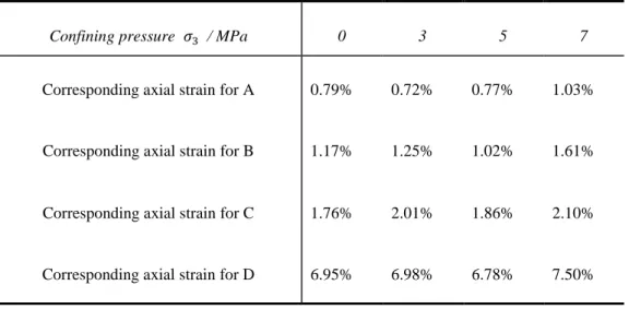
The stress-strain curves have similar characteristics of stages. The axial strains corresponding to the indicated points (see table 2.1) are similar. Point A represents

Corresponding axial strain for D 6.95% 6.98% 6.78% 7.50%

With the increasing confining pressure, the constants change: both the elastic modulus and Poisson’s ratio increase; the compression strength has a remarkable rise. The axial strain corresponding to the peak stress also increases significantly (see table 2.2). All the data are obtained at room temperature 26-30℃ and with the loading velocity of 0.2KN/s.

Table 2.2 Variation of elastic parameter with confining pressure

Confining pressure / MPa 0 3 5 7

Elastic Modulus E / GPa 6.50 7.40 8.10 8.65 Possion’s ratio 0.07 0.11 0.14 0.16 Compression strength / MPa 47.1 75.2 89.3 106 Axial strain corresponding to 8.92% 19.93% 25.3% 29.1%

mainly deformed, without visible macrocracks on the surface (Fig. 2.18). After point D, the macrocracks initiate, propagate and connect, forming the cracks (Fig. 2.19).

Dislocation theory is proposed to explain the plastic deformation. Fig. 2.20 shows the deformation process of an intact crystal lattice overcoming slip resistance under the drive of shear stress.

Fig.2.20 Sliding in the crystal lattice under shear stress

Edge dislocation is an extra half atomic planes during gliding process, typical of dislocation, as shown in Fig. 2.21. Two categories of edge dislocation are positive and negative.

Fig.2.22Screw dislocation

As the dislocations exists in the crystal, the atoms around the dislocation line deviate from the normal position, causing the lattice distortion and generating stress field. The stress state of that area removed the center region could be solved through the elastic theory. Dislocations cause the lattice distortion, leading to energy rise. The energy increment belongs to the dislocation strain energy, including elastic energy and core energy at the dislocation core.

Some vacancy condensation could occur during crystallization, forming dislocation sources. Three mechanisms for dislocation formation are formed by homogeneous nucleation, grain boundary initiation, and interfaces the lattice and the surface, precipitates, dispersed phases, or reinforcing fibers. Under the stress, dislocation source in the stress concentration area would ceaselessly emit dislocations to the glide direction. Once encounting obstacles, such as impurity atom, crystal boundary and subboundary, dislocations are impeded and stop gliding. As the following dislocations come, dislocation would pile up and the stress field would add together. To continue the

subjected to shear stress, the sample surface was polished and then soaked in the glacial acetic acid 15 min. the observed slip lines are shown in Fig. 2.23.

Fig.2.23 Dislocation slide lines in the salt materials

The process of loading on the samples actually is an interactive process between dislocations and external force. There are numerous pores and microcracks inside the natural rock salt. In the compaction stage, salt is subjected to the external force, the original cracks are compacted while the lateral strain does not occur, this corresponds to the nonlinear elasticity, since the lateral stress is fixed. In this phase, stress concentration usually occurs around the crack tips, where the dislocation sources are activated to emit dislocation, leading to irreversible deformation. Therefore the

After point D, the number of plied-up dislocations comes to a critical limit. Cracks start to propagate and connect generating volume increase. In this stage, the volumetric

strain increases rapidlyin a geometric progression. As the lattice structures are distorted

to a limit, some impurity atoms would separate out from the lattice, forming second phase. The second phase would further impede the dislocation and increase the internal stress. The cracks reduce the effective bearing area. When the average stress applied on the effective bearing area is large enough to destroy all the rest bearing element, the peak stress arrives. After peak, the cracks continue propagating and effective bear element continue reducing, resulting in a larger stress concentration.

As the salt samples are confined, crystal boundaries are protected better, needing more energy to open. More dislocations would traverse the crystal boundary. Therefore the plastic deformation is larger under larger confining pressure.

2.5 Chapter summary

In this chapter, the dislocation theory is used to explain the behavior of salt under continuous compression. In the uniaxial compression tests the deformation is mostly plastic, the elastic deformation being very small. The dilatancy behavior of salt could be understood considering three mechanisms and four stages.

Three mechanisms:

Compaction: at lower stress, the pores are compacted.

The process of loading on the salt actually is an interactive process between dislocations and external force (see section2.4.2). In triaxial compression tests, as the confining pressure increase,

①Elastic modulus and Poisson’s rate as well as the strength increase with the

confining pressure .

②Dilatancy difficulty increases and dilatancy angle decrease.

③Crystal boundaries are fortified and more dislocations could traverse the

In previous chapter, we analyzed the elastoplastic deformation in conventional compression tests. It is known however, that the information obtained from the laboratory tests is limited and should be generalized by constitutive modeling.

3.1 Elastic framework

Elastic deformation is reversible, identified from unloading process. The unloading curve is found not a straight line and does not overlap with the previous loading curve, forming a hysteresis loop (Fig. 3.1). Compared to the total deformation, the hysteresis loop is small, the unloading curve is a line and overlaps with the previous loading curve. Therefore, the elastic behavior could be described by Hook’s Law.

Plasticity of material could be caused by shear stress, creating volumetric expansion or contraction. Hydrostatic stress although cannot generates plastic strain, influences the development of plasticity, which must be taken into account in the elastoplastic constitutive model.

Geomaterials usually obey the non-associated flow rule (non-orthogonal flow rule), meaning that the inelastic incremental strain vector does not coincide with the normal to the yield surface. Increment constitutive relation in non-associated flow rule is

(3.3)

where is the plastic potential function. Plastic strain increment could be decomposed

into and . Since the Lode angle (the 3rd stress tensor invariant is neglected,

Equation (3.3) also can be rewritten as.

( ̅ ̅ ) (3.4) Where ； , ̅ √ √ (3.5)

Then, the plastic strain increment is

( _{√ ̅}) (3.6)

Plastic volumetric strain increment

(3.7)

̅ (3.10a)

(3.10b)

is plastic factor, a nonnegative scalar. Substitute equation 3.10a into 3.10b，

_̅ 𝐼 ̅ (3.11)

where is the dilatancy factor (function). Positive dilatancy factor means

volume increase, the negativefactor, means volume reduction or compaction.

3.3.1 Yield function

and are axial strain and lateral strain. 𝐿 𝐿； 𝐿 is the sample

shortening measured during the tests, L is the length of the smaple. ,

is the elongating of extensometer twining around the sample surface, R is the radius of the sample. Generilized shear strain and the plastic shear strain increment are calculated by

̅ √𝐽 _√ (3.12)

̅ ̅ 𝐺 (3.13)

The strain hardening appears during the loading process. Yield stress changes with the hydrostatic stress and plastic shear strain. Taking the values of yield stress and hydrostatic stress at the same plastic shear strain, the relationship between yield stress and hydrostatic stress could be obtained. Then the (undetermined) coefficients in the different yield stress-hydrostatic stress relationships are written as the functions of

Fig.3.2 Relationship between yield stress and hydrostatic stress under different ̅ . The quadratic function was employed in fitting the limited data from one uniaxial test and three triaxial tests, which has been shown in Section 2. The black cross represents the value where the samples fail.

̅ ̅ and ̅ take the values in Table 3.1。

Table3.1 Taking value for the functions ̅ ， ̅ and ̅

̅ ̅ ̅ ̅ 0.15 -0.0032 -0.6414 4.6 0.13 -0.0035 -0.6521 4.4 0.11 -0.0039 -0.6644 4.2 0.09 -0.0042 -0.6628 3.8 0 25 0 60 120 180

I

/MPa

a

Fig.3.3 Fitting the parameters to obtain the function of ̅ ̅ and ̅ .

By fitting the data, ̅ ， ̅ and ̅ are obtained

,

̅ ̅

̅ ̅

̅ ̅

(3.15)

Combining equation 3.10, 3.14, 3.15, the yield function is

𝐹 ̅ ( ̅ _{)𝐼 ̅ 𝐼 ̅ (3.16)}

3.3.2 Dilatancy function (plastic potential function)

Plastic potential function is defines the direction of incremental plastic deformation vector, or the value of dilatancy factor. Plastic volumetric strain is calculated as

𝐼 (3.17)

As stated in chapter 1, point D (in Fig. 2.12~2.17) is the critical point, after which third dilatancy mechanism (microcracks) would take effect and the volume expands

exponentially. Fitting the corresponding values of D points with R² = 0.9877, obtain

√𝐽 𝐼 9 (3.18) To simplify the model, the critical point is neglected. In Fig. 3.4, the

relationship between dilatancy factor and hydrostatic pressure is linear as ̅ is

unchanged.

Fig.3.4 Dependence of dilatancy factor on plastic shear strain and hydrostatic pressure.

̅ and ̅ are the function of ̅ , whose taking values are in Table 3.2。

Table3.2 Taking value for the functions ̅ ， ̅

̅ ̅ ̅

0.1 -0.0109 1.1112

0.08 -0.0107 1.0242

0.06 -0.0104 0.945

Fig.3.5 Fitting the parameters to obtain the function of ̅ ， ̅ .

a

3.4 Comparison of constitutive model to experimental data

Since the parameters are determined by fitting the experimental data, it is meaningless to verify the model by the used experimental data. This section will compare the constitutive model and the measured data in chapter 2 and show the difference.

3.4.1 Yield function

Plot of the yield function (3.16) is shown in Fig. 3.6. This figure intuitively shows the change in yield stress over plastic shear strain. In physics, the model includes the strain hardening.

Fig.3.7 Yield Function measured in compression test with different confining pressure.

Within the range of the measuring device, the measured maximal yield stress (Fig.

3.7) are 28.3 MPa ( ̅ ), 39.7MPa ( ̅ ),

42.1MPa ( ̅ ) and 43.3MPa ( ̅ ). Plotting the

loading path on the yield surface (Fig. 3.8), the maximal yield stress predicted by model are 26.5MPa, 39.2MPa, 41.9MPa and 42.9MPa respectively. The relative error between the two are 6.4%、1.3%、0.5%, 1.2%。

Uniaxial compression experimental results are easily affected by defects of samples, and have a relatively high random error. The results obtained from model are consistent with those from triaxial compression tests, indicating the model have good quality of describing the yield stress of salt, to some degree.

(c)

(b)

(d)

Fig.3.10 Dilatancy function and loading path in stress-strain space.

3.5 Chapter summary

This chapter transforms plastic potential function into dilatancy function, simplifying the formulation of plastic constitutive model. Considering the effect of hydrostatic stress and loading history, the yield function F based on the form of quadratic function and dilatancy function bases on the linear function are developed. The consitituve model could describe the strain hardening effect.

𝐹 ̅ ( ̅ _{)𝐼 ̅ 𝐼 ̅ (3.23a)}

( 9 _̅ ) 𝐼 _̅ (3.23b)

Based on the experiemental results, the failure criteria for salt was also developed, laying a fundament for furture data simulation.

4.1 Experimental design

The samples and the device used in the fatigue tests are the same as in the previous experiments. The experimental scheme is the following:

These series of fatigue tests are uniaxial or triaxial cyclic loading tests. Considering the compression strength obtained before, upper and lower stress limits are determined to conduct the fatigue tests. The tests are divided into 4 groups named 1201a group, 1201b group, 1201c group and 1201d group, to investigate the stress effect, loading velocity effect, temperature effect and confining pressure effect, respectively. 1201a group have two subgroups, 1201a1 and 1201a2, for upper stress limit and lower stress limit. All the tests adopt the velocity of 0.2KN/s to load to the target stress, then apply the designed velocity.

1201a1 group tests hold the lower stress limit constant, 9.4MPa, 20% of the uniaxial compression strength; upper stress limit is 95%, 90%, 85%, 80% of the uniaxial compression strength. Room temperature is 25±2℃; Air humidity is 57±5%; Loading velocity is 2KN/s.

1201a2 group tests hold the upper stress limit constant, 90% of the uniaxial compression strength; lower stress limit is 20%, 30%, 40%, 50% of the uniaxial compression strength. Room temperature is 25±2℃; Air humidity is 57±5%; loading velocity is 2KN/s.

4.2.1 Stress limit effect

Stress ratio is the ratio of the stress limit (the maximum stress or minimum) to the strength. The effect of stress limit on the fatigue has been investigated by many authors. Here just briefly verify the effect on salt fatigue. In 1201a1 group, as the upper (stress) limit decreases from 95% to 90%, 85% and 80%, the fatigue life increases from 26 to 68, 205 and 582 (Fig. 4.1), showing that the decreasing upper limit could augment the fatigue life with the lower limit constant.

(b) Axial stress vs axial strain in cyclic loading test with 20%~90% stress limit

(d) Axial stress vs axial strain in cyclic loading test with 20%~80% stress limit. Fig.4.1 Axial stress vs axial strain curves with different upper stress limits.

With the constant upper limit of 90%, the fatigue life changes from 68, to 85, 42 and 374, respectively, as the lower limit increases from 20% to 30%, 40% and 50%. As an overall trend, the fatigue life augments with the lower limit reduction. It can be found from the loading-unloading curves that the yield stress in the reloading process is close to previous upper limit, 3~5 MPa below the upper limit stress. Since the lower limit just changes below the yield stress, the plastic deformation should not show any difference. In my opinion, the fatigue life changes for other than the yield stress reason. In subsequent section, the reason will be revealed.

One point need note is that the total deformation of sample of 1201a2 group is in positive relation with fatigue life. 68 to 11.6%, 85 to 12.3%，42 to 9.1%，374 to 14.1%.

4.2.2 Loading velocity effect

Numerous researches show that loading frequency could enhance the rock sample’s strength, thus augment the fatigue life. However, within our testing range, the loading frequency has no remarkable effect on the salt fatigue. In 1201b group, loading velocity increases from 0.36KN/s to 10KN/s, the fatigue life just fluctuates slightly.

5 23 10 2300

3 49 9.5 5000

1 23 10.4 5200

0.36 38 12 18000

4.2.3 Temperature effect

Every uniaxial compression test with different temperature is conducted more than three times. The results show that the temperature exerts a notable influence on the salt compression strength. As shown in Fig. 4.2, the strength reduces from 47.1MPa to 40MPa with the temperature increasing from 13℃ to 60℃.

(a) Cyclic loading-unloading test at 13℃

(c) Cyclic loading-unloading test at 60℃

Fig.4.3 Axial stress-axial strain curves from uniaxial compression and fatigue tests at different temperature.

4.2.4 Confining pressure effect

The strength of salt increases with the mean stress or confining pressure. For the salt, the confining pressure enhances the deformability as well. As shown in Fig. 4.4, the compression strength increases from 47.1MPa to 89.3MPa and the total deformation prior the failure increases from 8.92% to 25.3%. However, it is unclear whether the confining pressure could influence the salt fatigue for the same stress ratio, . 1201d group is to work out this.

σ3=0

σ3=3MPa

(c) Axial stress vs axial strain in cyclic loading test with 5MPa confining pressure Fig.4.5 Axial stress-axial strain curve from fatigue tests at different confining pressure.

4.3 Fatigue life model based on energy dissipation

The product of stress and time is defined as stress energy 𝐸_𝑤, in stress

unloading-loading cycle

𝐸𝑤 𝑇 𝑇 𝑇 𝑇 (4.1)

𝑇 and 𝑇 are the loading time and unloading time, is lower stress limit,

is stress ampulitude. Loading with constant velocity,

𝑇 𝑇 (4.2)

Substitute equation (4.2) into equation (4.1),

𝐸_𝑤 (4.3)

There are three stages in fatigue deformation: decelerating deformation stage, uniform deformation stage and accelerating stage. If the stress ratio is smaller, the uniform deformation stage amounts for a greater proportion of total deformation. In uniform deformation stage, every residual strain keeps roughly constant. Supposed that

fatigue life and upper stress limit is exponential function. Viscocity coefficient of rock

usually is 1019~1023Pa.s. Here taking 1020Pa.s for the viscosity coefficient, 𝐶

_{, 𝜍 .}

𝜍 _{𝐶 (4.8)}

Fig.4.6 N-S curve under different upper limit stress.

In this model, temperature and confining pressure can change the fatigue life through the viscosity coefficient.

nearly the same with different confining pressure and stress ratio.

(b) Confining pressure = 3MPa

(c) Confining pressure = 5MPa

Fig. 4.7 Axial stress-plastic axial strain curve from compression fatigue tests.

Fig. 4.8 Shear stress-plastic shear strain curve of uniaxial compression test and unloading test.

4.4.2 Yield function in reloading

Weakening coefficient χ is introduces to characterize the difference between the

two curves in YR segment in Fig. 4.9, 2 representing the second stress cycle

χ ̅ _̅ ̅ (4.9)

̅ is the shear stress in reloading; ̅ is the shear stress in uniaxial compression

Y

R

U

2

Fig. 4.9 Values taken by weakening parameter χ .

By fitting, χ obtain

χ _γ

Y𝑅

(4.11) The yield function in reloading is

𝐹 _χ ̅

𝐹 𝐼 (4.12)

4.4.3 Dilatancy function in reloading

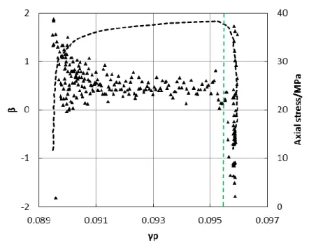
Comparing the monotonous compression test and cyclic loading test, the dilatancy factor does not show big difference. In every reloading, the factor fluctuates around a constant level (Fig. 4.10). At first, the fluctuation range is large, then lessen. On the whole, the dilatancy function of constitutive model in reloading can be considered to be the same as for the continuous loading.

However, if we look into more details, it can be found that the dilatancy factor actually is bigger in the beginning and then decreases to a constant. It is interesting that the plastic deformation develops due to the micro-cracking at the beginning of reloading and then due to the dislocations.

Fig. 4.10 Comparison of dilatancy factor between uniaxial test and fatigue test.

4.4.4 Strengthening coefficient and loosing zone

For the cyclic loading, no matter metal material or geomaterial both use dynamic

model to modify the yield function [122-129]. The yield function in third loading could be

considered as the translation of that in second loading, and so on. Therefore, the yield function in cyclic loading is

𝐹 _χ ̅

(𝐼 ∑ = ) (4.13)

χ _γ

Y𝑅 (4.14)

𝑅 𝑌 , very important to the modified yield function, could be understood as

the influence range of self-weakening and denoted as loosing zone. Its dimension is decided by the residual stress remaining after unloading. By far there is bare relevant research reported. Here, the loosing zone is assumed as a function of the loading history

(the residual strain _𝑅) and stress state.

Y𝑅 Y𝑅( ̅ 𝐼 𝑅) (4.15)

4.5 Chapter summary

This chapter investigated the conventional fatigue properties of rock salt with different stress ratio, loading velocity, temperature and confining pressure. Experimental results showed that:

Upper limit increase the fatigue life, while lower limit did not have significant impact on the fatigue life.

Loading velocity (with the range of 0.36KN/s~10KN/s) does not affect notably the fatigue life.

The rising temperature (within the range of 13℃~60℃) can lightly increase the fatigue life.

Under the same stress limits, confining pressure significantly raise the fatigue live, because the tenacity is strengthening.

A fatigue life model based on energy dissipation theory is established. Temperature and confining pressure can change the fatigue life through viscosity coefficient. Stress ratio changes the fatigue life by plastic work.

𝜍 𝐴

(4.18) Through dislocation theory, the variation of dilatancy factor could reflect the development of dislocations and microcracks. In fatigue tests, the dilatancy factor increases with the cycle number, indicating that the contribution of microcracks to dilatancy growth. Inside the cycles, the dilatancy factor is initially big and then

cycle does not continuously change, but discontinuously changes, Fig. 5.1.

means the balance of supply and demand. The gas pressure keeps constant.

Fig.5.2 Gas consumption for one city in China.

Germany Huntorf plant completes one cycle every day. The underground salt CAES works 10 hours and stop 14 hours. During the period of stop, the air pressure inside CAES is constant. Whether this pressure plateau would exert influence on the fatigue properties is unclear.

Fig.5.3 Sample encased in a plastic fresh-keeper bag.

Three groups of discontinuous cyclic loading tests, 1301group, 1401group and 1501group, are conducted to investigate the basic properties of discontinuous fatigue, the effect of time interval and the effect of lower stress limit, respectively.

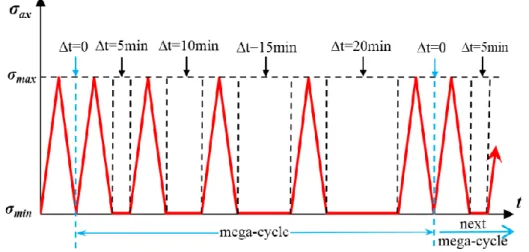
To eliminate the possibility of creep, the lower stress limit is set at zero in group 1301. Regarding the sensitivity of the loading machine, it is difficult to reach real 0KN, the stress limit is set to 3KN. To control the experimental time within 0.5~2hour, the upper (stress ratio) limit is set to 85%. The loading velocity is 2KN/s. After every two continuous cycles the loading is interrupted during a certain time interval (Fig. 5.4). The cycles before these intervals are denoted as B path, while the after, they are denoted as A path.

Fig.5.4 Loading path for 1301group tests.

5.2 Essential features

5.2.1 Stress-strain curves

Discontinuous fatigue tests show a distinct difference from the conventional tests. As shown in Fig. 5.5, the fatigue life of the salt samples from conventional fatigue test and 1301group tests are 89, 34, 24, 13, 20, respectively. The fatigue live of salt from 1301group is significantly lower than that from the conventional one under the same conditions.

(b) Discontinuons fatigue test (∆t=5min)

(e) Discontinuons fatigue test (∆t=20min)

Fig.5.5 Axial stress-axial strain plot from conventional fatigue test and 1301.group of discontinuous fatigue tests.

Calculating the total accumulated plastic deformation (except the last uncomplete cycle), this accumulated plastic deformation of the salt samples from 1301group is 7.2%-8.5%, smaller that from conventional fatigue tests, 9.1%-11%.

5.2.2 Residual strains

Every loading generate a certain deformation. While one part of it (elastic deformation) is recovered during the unloading, the other, is not. The remaining part is

plastic strain, also called the residual strain , where i represents the cycle number.

Calculating the residual strain in every cycle leads to the understanding of the evolution of plastic damage of salt sample under discontinuous cyclic loading. Fig. 5.6 shows the residual strain evolution with stress cycles. The residual strain firstly reduces, then keeps at a constant and finally increases a little when close to failure. In previous studies, the first stage is called as decelerated deformation phase; the second is uniform

deformation phase; the last is accelerated deformation phase [126]. In the aspects of these

three phases, 1301group tests show the same features with the conventional.

However, what is the distinct between two types of fatigue tests is that: In 1301group tests, the residual strain from A path is significantly larger than that from B path. Fig 5.7 accumulated the residual strain separately for A path and B path. It can be

(a) Conventional fatigue test

(d) Discontinuons fatigue test (∆t=15min)

(e) Discontinuons fatigue test (∆t=20min)

Fig.5.6 Evolution of the residual strain with loading cycles from conventional fatigue test and 1301.group of discontinuous fatigue tests.