HAL Id: hal-01609107
https://hal.archives-ouvertes.fr/hal-01609107
Submitted on 6 Nov 2018HAL is a multi-disciplinary open access
archive for the deposit and dissemination of sci-entific research documents, whether they are pub-lished or not. The documents may come from teaching and research institutions in France or abroad, or from public or private research centers.
L’archive ouverte pluridisciplinaire HAL, est destinée au dépôt et à la diffusion de documents scientifiques de niveau recherche, publiés ou non, émanant des établissements d’enseignement et de recherche français ou étrangers, des laboratoires publics ou privés.
An analytical model for the prediction of hot roll
temperatures in a hot rolling process
Vincent Velay, Abderrahim Michrafy
To cite this version:
Vincent Velay, Abderrahim Michrafy. An analytical model for the prediction of hot roll temperatures in a hot rolling process. Materials Science and Engineering Technology / Materialwissenschaft und Werkstofftechnik, Wiley-VCH Verlag, 2016, 47 (12), p. 1202-1215. �10.1002/mawe.201600554�. �hal-01609107�
An analytical model for the prediction of hot roll
temperatures in a hot rolling process
Vorhersage der Warmwalztemperatur in einem Warmwalzprozess
durch ein analytisches Modell
V. Velay1, A. Michrafy2
Temperature variations in the hot roll during a hot rolling process were analysed by solving heat conduction equations for boundary conditions using an analytical meth-od. The analysis was conducted in a steady-state regime, taking into account the effects of process parameters such as the contact surface, roll velocity and various cooling boundary conditions. Assuming the periodicity of the process, the develop-ment of a solution in the Fourier series was employed to solve the governing equa-tions. The temperature and its gradient distributions in the roll depth were analyti-cally expressed according to the process parameters. The accuracy of the predicted results was examined through comparison with predictions presented in the litera-ture (finite element solutions and measurements). Results showed that an increase in the rolling speed leads to a shorter contact time, which decreases the temperature field in the work-roll.
Keywords: Hot rolling process / thermal transfer / process parameters
Schlüsselwörter: Warmwalzprozess / Wärmeübergang / Prozessparameter
1 Introduction
The hot rolling process is an important industrial process for manufacturing sheets with the appropri-ate mechanical properties. In this process, the work-rolls are subjected to severe and periodic thermal loading during contact with the hot strip [1]. The re-peated thermal cycles are responsible for the failures observed on the roll surface [2–7]. These failures are essentially a consequence of the thermal gradient, resulting from the heat transfer in the contact zone between the strip, where the temperature can reach 1273 K (1000°C), and the external cooling
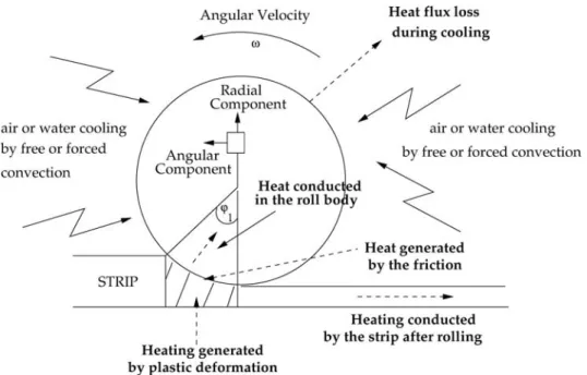
condi-tions applied on the roll [8]. In addition to the differ-ence in temperature between the strip and the roll, plastic strains generated by pressure applied by the roller and frictional conditions required for success-ful hot rolling cause a rise in the temperature at the contact surface [9, 10]. The changing conditions of heating and cooling operations are of considerable importance, since they reduce the lifetime of the work-roll, which is continuously subjected to ther-mal gradients generating high therther-mal stresses. Fig-ure 1 summarizes the various heat flows generated in a hot rolling process from the heat exchange in the contact zone between the strip and the roll and the heat lost by air or water spray cooling. With the aim of increasing the lifetime of the roll, it is
essen-Corresponding author: Vincent Velay, Université de Toulouse – CNRS, Mines-Albi, INSA, UPS, ISAE-SUPAERO; ICA (Institut Clément Ader), Campus Jar-lard – 81013 Albi – Cedex 09 – France,
E-Mail: [email protected]
1 Université de Toulouse – CNRS, Mines-Albi, INSA,
UPS, ISAE-SUPAERO; ICA (Institut Clément Ader), Campus Jarlard – 81013 Albi – Cedex 09 – France
2 Laboratoire de Génie des Procédés des Solides
Di-visés – UMR CNRS 2392, Ecole des Mines d’Albi-Carmaux, Campus Jarlard – 81013 Albi Cedex 09 – France
tial to know the temperature distribution in the work-roll during the hot work-rolling process. Several studies have been conducted to calculate temperature distri-bution in the work-roll using numerical, semi-analy-tical and analysemi-analy-tical techniques [11–17]. The main advantage of the finite element method is to solve the governing heat-conduction equations for both the strip and the work-roll simultaneously [14, 18]. However, this technique requires fine meshes near the contact zone and hence high CPU time, which makes it difficult to use as an on-line process control method.
In contrast, the analytical solution seems to be more suitable for providing closed form equations for the temperature field and thermal stresses which compute very efficiently [12].
In this investigation, the contact between the roll and the strip is assumed perfect and the heat transfer generated by both plastic deformation of the strip and by friction is taken into account through a global contact temperature. Unlike several other studies the strip is not explicitly considered and the analysis of the heat transfer is focused only on the roll [9, 10, 19–21]. The analysis is based on the temperature of the contact surface, the process parameters, such as the angular velocity ω, the entry thickness of the strip – which corresponds to theφ1angle – and
var-ious cooling boundary conditions denoted by theφ2
angle.
The objective of this work is to develop a semi-analytical formulation of the heat transfer in the roll during the hot rolling process with accurate and ap-propriate time computation. In addition, this devel-opment could be used as a predictive tool for the optimization of the hot rolling process. The type of solution will strongly depend on the process para-meters considered (cooling conditions, angular velo-city of rotation) [22–24].
2 Heat equation and boundary conditions The heat transfer equation in the roll during hot roll-ing is described by Eq. (1).
dT
dt ¼aΔT ð1Þ
where a ¼ λ
ρCp is the thermal diffusivity and λ, ρ
and Cpare respectively the thermal conductivity, the
density and the specific heat of the material.
The stationary state leads to the following rela-tion: dT dt ¼ @T @φ φ ¼_ @T @φ ω ð2Þ
Thus, the assumption of Eq. (2) combined with Eq. (1) expressed in a polar coordinate system pro-vides the following relation:
@2T @ξ2 þ 1 ξ2 @2T @φ2þ 1 ξ @T @ξ% ωR2 a @T @φ¼ 0 ð3Þ The temperature field will depend on the angle φ 2 0; 2π½ ' and a dimensionless radius ξ 2 0; 1½ ', de-fined as the ratio between r and the radius of the roll R, with 0 ( r ( R. Various boundary conditions are considered along thesurface of the roll. They can greatly influence the temperature field within the body of the roll. On the first part, delimited by angle φ1, an applied temperature is considered (Dirichlet
condition), which reproduces the temperature of the strip. Consequently, the angle φ1 is considered as
the contact arc length between the roll and the strip. On the remaining part of the roll, different cooling conditions can be applied (Neumann boundary con-ditions). For instance, the roll can be cooled by water or by air jet. Depending on the industrial pro-cess, these kinds of cooling can occur separately, or both of them may be be used in conjunction. In this last case, another angleφ2is introduced to define the
part of the roll surface cooled by water jet and the part cooled by air jet.
Finally, both boundary conditions (Dirichlet and Neumann conditions) can be illustrated as:
ξ ¼ 1; β φð Þ @T@ξþ T % θ φð Þ ¼ 0 ð4Þ where: β φð Þ ¼ 0 if 0 ( φ ( φ1 λ Rhð Þφ if φ1( φ ( 2π 8 < : and: θ φð Þ ¼ θ1 if 0 ( φ ( φ1 θ2ð Þ if φφ 1 ( φ ( 2π (
θ1is the applied temperature, selected so as to be
close to the strip temperature. θ2(φ) is the
tempera-ture of the cooling fluid (water or air). Its value is constant if only one kind of cooling is considered, but it can evolve with φ, φ1 ( φ ( 2π if several
kinds of cooling are applied. The thermal exchange coefficient is represented by h(φ). Its value will strongly depend on the cooling conditions (fluid and rate).
3 Temperature as Fourier series development
The periodicity aspect of problems (3) and (4) re-quires us to seek the solution as a development of the Fourier series [25, 26]. The temperature field can be then written as:
Tðξ; φÞ ¼ X N n¼%N Tnð Þ eξ inφ ð5Þ where: Tn 2 ℂ and T%n ¼ Tn Tn is the conjugate of Tn i is such that i2 ¼ %1 and N ! 1:
In fact, the numerical implementation requires an integer value for N. This point will be discussed later in the paper.
Introducing Eq. (5) into Eq. (2) and considering all the terms of the Fourier series, the following equations are obtained:
@2Tn @ξ2 þ 1 ξ @Tn @ξ % n2 ξ2þ i ε2 n ! " Tn¼ 0 ð6Þ where: 1 εn ¼ R ffiffiffiffiffiffi nω a r 8n ¼ )1; . . . ; )N
It is obvious that the solution of the ordinary dif-ferential Eq. (6) is provided through a Bessel func-tion Jnof the first kind of order n. Indeed, the func-tion Tn(ξ) can be written as:
Tnð Þ ¼ Aξ nJn ξ 1 % ið ffiffiffi Þ 2 p εn ! " where Anis a constant.
Moreover, an asymptotic expression of the Bessel function leads to the following form of the equation [27]: Tnð Þ ¼ξ τn ξ e 1þi ð Þ ξ%1ffiffið Þ 2 p εn ð7Þ
where:τn 2 ℂ and its conjugate τn ¼ τ%n.
Hence, the computation of Tn results from the
determination ofτn. Representingβ(φ) and θ(φ) (see
Eq. (4)) in terms of the Fourier series:
β φð Þ ¼ X N n¼%N βneinφ; θ φð Þ ¼ XN n¼%N θneinφ ð8Þ
and including Eq. (8) into the boundary condition Eq. (4), we obtain the Eq. (9) that includes the boundary conditions. XNþn j¼%Nþn βj @Tn%j @ξ þ Tn% θn ¼ 0; ξ ¼ 1 ð9Þ 8n ¼ 0; )1; . . . ; )N
Then, using Eq. (7) in the previous Eq. (9), the following form can be found:
Xn%1 j¼%Nþn τn%jβj 1 þ iffiffiffi 2 p εn%j% 1 2 ! þ X Nþn j¼nþ1 τj%nβj 1 % iffiffiffi 2 p εj%n% 1 2 ! þ τn% θn%12τ0βn¼ 0 ð10Þ
More details are given in appendix A.
Consequently, the computation ofτnfrom Eq. (10)
completely determines the temperature field. How-ever, this determination requires knowledge of θn andβn, which can be derived from the Fourier Series properties (2π periodicity) of θ(φ) and β(φ).
θ φð Þ ¼ X N n¼%N θneinφ where: θ0 ¼21 π ðθ1φ1þ θ2ð2π % φ1ÞÞ θn ¼21 πn ðθ1% θ2Þðe%inφ1% 1Þ i 8 > > < > > :
in the case where one type of cooling condition is applied: β φð Þ ¼ X N n¼%N βn einφ where: β0¼2πRhλ ð2π % φ1Þ βn¼2 λ πRhn i 1 % e%inφ1 $ % 8 > > < > > :
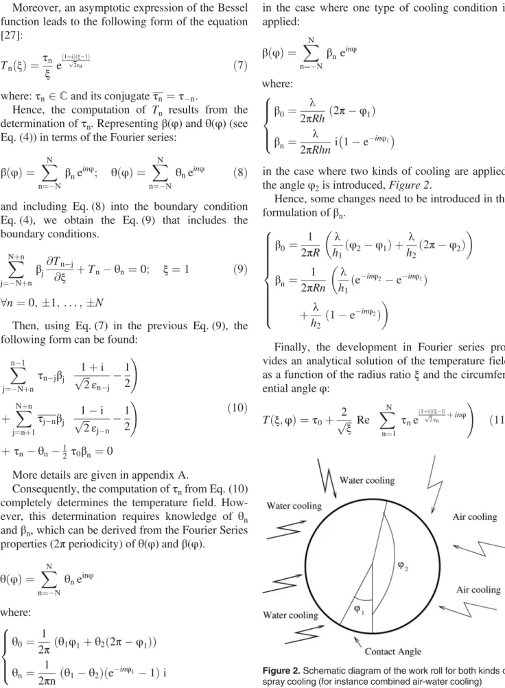
in the case where two kinds of cooling are applied, the angleφ2is introduced, Figure 2.
Hence, some changes need to be introduced in the formulation ofβn. β0¼ 1 2πR λ h1ðφ2% φ1Þ þ λ h2ð2π % φ2Þ ! " βn¼ 1 2πRn λ h1ðe %inφ2 % e%inφ1Þ ! þhλ 2 ð1 % e %inφ2Þ " 8 > > > > > > > > < > > > > > > > > :
Finally, the development in Fourier series pro-vides an analytical solution of the temperature field as a function of the radius ratio ξ and the circumfer-ential angleφ: Tðξ; φÞ ¼ τ0þp Re2ffiffiffiξ XN n¼1 τne 1þi ð Þ ξ%1ffiffið Þ 2 p εn þ inφ ! ð11Þ
Figure 2. Schematic diagram of the work roll for both kinds of spray cooling (for instance combined air-water cooling)
Where Re (z) is the real part of the complex num-ber z.
Following on from this, the thermal gradient dis-tributions can be computed by derivation from the previous equation: @T @r ðξ; φÞ ¼ 2 R ffiffiffip Reξ XN n¼1 τn 1 þ iffiffiffi 2 p εn% 1 2ξ ! " * eð1þipÞ ξ%1ffiffi2ðεn Þþ inφ " @T @φ ðξ; φÞ ¼ 2 ffiffiffiξ p Re X N n¼1 inτne 1þi ð Þ ξ%1ffiffið Þ 2 p εn þ inφ !
More developments are given in appendix B.
4 Numerical implementation
The objective of the numerical procedure is to com-pute the temperature field T and its gradient in the hot roll during the hot rolling process. This consists in the computation of τi; i¼ 0; )1; . . . ; )N from
the system of equations described below.
The objective of the numerical implementa-tion is to evaluate Eqs. (7) and (10). The main difficulty is then to calculate the coefficient τn8n ¼ 0; )1; . . . ; )N. For this purpose, Eq. (10)
is re-written under a matrix form which leads to the following relation: n ¼ 0: βð %NαNτNþ . . . þ β%1α1τ1Þ þ βð 1α1τ1þ . . . þ βNαNτNÞ þ τ0%τ2 β0 0¼ θ0 .. . .. . n ¼ N: βð 0αNτNþ . . . þ βN%1α1τ1Þ þ β$ Nþ1α1τ1þ . . . þ β2NαNτN%þ τN%τ2 β0 N ¼ θN with: αn ¼ 1 þ iffiffiffi 2 p εn% 1 2
The system could be written in matrix form, such as: %β20 α1β%1 . . . αNβ%N .. . .. . . . . .. . %β2N α1βN%1 . . . αNβ0 0 B B B B B B @ 1 C C C C C C A |fflfflfflfflfflfflfflfflfflfflfflfflfflfflfflfflfflfflfflfflfflfflfflfflfflfflfflfflffl{zfflfflfflfflfflfflfflfflfflfflfflfflfflfflfflfflfflfflfflfflfflfflfflfflfflfflfflfflffl} A τ0 .. . τN 0 B B B B @ 1 C C C C A þ α1β1 . . . αNβN .. . . . . .. . α1βNþ1 . . . αNβ2N 0 B B B @ 1 C C C A |fflfflfflfflfflfflfflfflfflfflfflfflfflfflfflfflfflfflfflfflfflffl{zfflfflfflfflfflfflfflfflfflfflfflfflfflfflfflfflfflfflfflfflfflffl} B τ1 .. . τN 0 B B B @ 1 C C C A |fflfflfflffl{zfflfflfflffl} ! τ þ τ0 .. . τN 0 B B B @ 1 C C C A¼ θ0 .. . θN 0 B B @ 1 C C A where: A 2 MNþ1; Nþ1ð Þ; B 2 Mℂ Nþ1; Nð Þ;ℂ τ; !τ 2 ℂN; θ ¼ θ1 .. . θN 0 B @ 1 C A 2 ℂN We note: ~θ ¼ θ0 θ ! " 2 ℂNþ1; ~τ ¼ τ0 τ ! " 2 ℂNþ1; ~ ! τ ¼ τ!τ0 ! " 2 ℂNþ1; ~ B ¼ 0 .. . 0 B 0 @ 1 A 2 MNþ1; Nþ1ð Þℂ
Knowing that ~B!~τ ¼ B!τ, the following linear sys-tem is obtained:
A þ INþ1
where A ¼ Re Að Þ þ i Im Að Þ ~ B ¼ Re ~B$ %þ i Im ~B$ % ~τ ¼ a þ ib; a; b 2 ℝNþ1 8 < : and a ¼ a0 .. . aN 0 B @ 1 C A; b ¼ b0 .. . bN 0 B @ 1 C A
In the previous system, Re (A) (respectively Im (A)) is the real part of the complex number A (respectively the imaginary part).
Equaling real and imaginary parts of the Eq. (12), it follows: Re Að Þ þ Re ~B$ %þ INþ1 $ % a þ Im ~B$ $ %% Im Að Þ%b ¼ Re ~θ$ % Im Að Þ þ Im ~B$ % $ % a þ Re A$ ð Þ % Re ~B$ %þ INþ1%b ¼ Im ~θ$ % and we note: C1¼ Re Að Þ þ Re ~B$ %þ INþ1 C2¼ Im ~B$ %% Im Að Þ C3¼ Im Að Þ þ Im ~B$ % C4¼ Re Að Þ % Re ~B$ %þ INþ1 8 > > > < > > > :
It results that the real and imaginary parts ofτ can be obtained from the linear system:
a b ! " ¼ CC1 C2 3C4 ! "%1 Re ~$ %θ Im ~$ %θ ! ð13Þ
Finally, an explicit formulation of the coefficient Akj(respectively ~Bkj) of the matrix A (respectively of
matrix ~B) completes the numerical implementation. From Eq. (12), we can write:
A~τ þ ~τ þ ~B!~τ
$ %
k ¼ ~θk 8k ¼ 1; . . . ; N þ 1
or under index form:
XNþ1 j¼1 ð~Akj~τjþ ~Bkj!~τjÞ þ ~τk¼ ~θk 8k ¼ 1; . . . ; N þ 1 with: Akj¼ % βk%1 2 ; 8k ¼ 1; . . . ; N þ 1; j ¼ 1 αj%1βk%j; 8 k; jð Þ ¼ 1; . . . ; N þ 1; j 6¼ 1 8 < : ð14Þ ~ Bkj ¼ 0; 8k ¼ 1; . . . ; N þ 1; j ¼ 1 αj%1βkþj%2; 8 k; jð Þ ¼ 1; . . . ; N þ 1; j 6¼ 1 8 > < > :
The different steps leading to the temperature field formulation are illustrated, Figure 3.
5 Results
Based on the previous numerical procedure, a pro-gram was developed under MATLAB software to solve the distribution of the temperature in the roll. This methodology can be applied to investigate the influence of several process parameters, like the strip temperature and the kinds of cooling employed. The thermo-physical properties of the roll material and the process parameters are given, Table 1.
Table 1. Process and physical properties
φ1= 12π/180 Contact arc length [rad]
R = 0.35 Roll body radius [m]
ω = 0.3 Angular velocity of rotation of the roll [rad/s] Cp= 510 Heat capacity [J/kg/K]
ρ = 7800 Density [kg/m3]
λ = 16 Thermal conductivity [W/m/K] θ1= 885(552) Strip temperature [K (°C)]
θ2= 293(25) Air or water temperature [K (°C)]
h = 1500 Forced air cooling thermal exchange coefficient [W/m2/K]
5.1 Number of terms in Fourier series
The first analysis is related to the number of terms N considered in the Fourier series in order to obtain re-levant results. A minimal number of terms of 3000 is required in order to reproduce the boundary condi-tions on the arc length in contact with the strip. The model response for different values of the parameter N is compared, Figure 4. A mean temperature of 824 K (551°C) is found close to those considered in the Dirichlet boundary condition intended to re-produce the strip temperature (T = 825 K (552 °C)).
However, smaller values are not suitable, because they induce an important drop in the temperature along the arc length, Figure 4.
All the results presented below are computed using N = 3000.
Different boundary conditions were applied and predictions of temperature profiles were examined in comparison with results using the Finite Element Method and measurements from [9, 28].
The evolution of the temperature versus the roll-ing angle for different thicknesses is shown,
Fig-Figure 3. Calculation stages of the temperature field
Figure 4. Influence of the number of terms in the Fourier series
ure 5. As can be seen, the temperature at the roll sur-face reaches 818 K (545°C) along the contact arc of 12°. Afterwards, the temperature decreases rapidly with the rolling angle. However, a little further from the surface (10 mm in depth), the temperature barely reaches 473 K (200°C). From this depth to the roll center, the temperature does not evolve any more. The obtained temperature profiles confirm the very localized heated zone on the roll and are in agree-ment with results obtained using the finite eleagree-ment method and available measurements [13, 19, 28]. However, the maximum temperature at the roll sur-face in the contact arc depends on the roll speed (contact time), the coefficient of heat transfer, the roll diameter (contact angle) and the thermo-physical properties of the roll material.
A comparison of the temperature evolution for three different spray cooling conditions was plotted (air or water spray cooling and a combined air-water cooling), Figure 6. For the air-water spray cool-ing, the model prediction shows a rapid decrease in the temperature from 833 K (560°C) down to 298 K (25°C), whereas a higher value (around 373 K (100°C)) was found in the case of air cooling.
The third case is a combination of air and water spray cooling. First, the air spray cooling is applied followed by the water spray cooling. The separation angle is equal toφ2¼ 90+Figure 6.
The temperature distribution obtained at the roll surface is quite close to the curve obtained with air spray cooling for the first part φ2¼ 90+) and
pre-sents a similar profile to the temperature distribution
in the water spray cooling case in the second part (90+ <φ
2 < 360+).
However, an offset of the curve is observed in the transition zone (air to water spray cooling).
5.2 Effects of process parameters on the temperature distribution
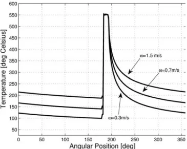
The distribution of the temperature in the roll de-pends on the process parameters, such as the roll pressure and roll diameter, both of which affect the contact arc, and is also dependent on the roll speed which determines the contact time and hence has an effect on the heat exchange conditions.
In the proposed modelling the temperature dis-tribution is directly expressed as a function of the process parameters (contact angle, angles where the spray cooling is applied and roll speed). In this mod-el the strip is only represented by the contact arc and heat exchange coefficient. The impact of roll pres-sure can be then appreciated through the contact an-gle.
To examine the influence of the contact angle and the roll speed on the maximum temperature and the heat flux on the roll surface, simulations were con-ducted by varying their values. Results are pre-sented, Table 2. These results indicate that the in-crease in the contact angle inin-creases the heat transfer between the strip and the roll. Furthermore, it is shown that a low roll speed favors the heat exchange from the strip to the roll, Figure 7. These results are consistent and supported by the general observations in the literature.
5.3 Impact of the contact conditions
The contact between the strip and the roll is not perfect in general. This is due to the existence of a thermal resistance Rc which limits the heat transfer.
In the previous results, the contact between the strip and the roll was assumed as a perfect contact, and was modelled as a Dirichlet condition. The new
Figure 6. Comparison of the temperature evolution for air or water spray cooling and for a combined air-water spray cool-ing
Table 2. Influence of the contact arc length on the mean temperature and on the thermal flux undergone by the roll Contact angle
[°] T[K (°C)]mean Thermal flux[W/m2]
5 807.5 (534.4) 3.3 × 10⁵
11.7 818 (545) 4.71 × 10⁵
boundary condition requires some changes in the model formulation by replacing Dirichlet with Neumann boundary conditions. The development of these changes is reported in Appendix C.
The temperature distribution from the roll surface is plotted for three thicknesses, Figure 8. The curves obtained have the same trends as the previous ones but the maximum temperature along the arc length is lower (T = 791 K (518°C)). Furthermore, it can be noted that the peak temperature has shifted towards the rotation direction in accordance with the depth [29]. This is essentially due to convection caused by the rotation of the roll.
6 Conclusion
In this work, an analytical methodology was devel-oped in order to assess the temperature field of work rolls during the hot rolling process. The model gives relevant results to predict the very high thermal gra-dient occurring at the surface of the roll body. This approach seems to be more suitable than a standard finite element calculation, which requires a very thin mesh close to the surface of the roll and conse-quently will require more time-consuming calcula-tions without ensuring good reliability. The present model considers a stationary thermal behaviour and does not take into account the transient phenomena. It allows several process parameters to be investi-gated, such as the arc length in contact with the strip, the angular velocity of rotation, or the cooling and heating conditions. Moreover, the number of terms considered in the Fourier series have to be carefully calibrated (N > 2000) in order to reproduce the boundary condition along the thermal contact. From this investigation, future work will seek to evaluate the stress levels within the rolls generated by the thermal gradient.
Appendix A
It is obvious that Eqs. (7) and (9) lead to the follow-ing form: X Nþn j¼%Nþn τn%jβj 1 þ iffiffiffi 2 p εn%j% 1 2 ! þ τn% θn ¼ 0 8n ¼ 0; )1; . . . ; )N
Moreover, the Fourier series properties give T%n ¼ Tnand thenτ%n ¼ τn.
Hence, the previous equation can be re-written as:
%12 τ0βnþ Xn%1 j¼%Nþn þ X Nþn j¼nþ1 ! * τn%jβj 1 þ iffiffiffi 2 p εn%j% 1 2 !! þ τn% θn ¼ 0 8n ¼ 0; )1; . . . ; )N
Figure 7. Influence of the angular velocity on the temperature distribution within the roll
Figure 8. Temperature evolution for different thicknesses within the roll in the case of a thermal contact resistance Rc=
where: XNþn j¼nþ1 τn%jβj 1 þ iffiffiffi 2 p εn%j% 1 2 ! ¼ X Nþn j¼nþ1 τj%nβj 1 þ i ipffiffiffi2εj%n% 1 2 ! ¼ X Nþn j¼nþ1 τj%nβj 1 % iffiffiffi 2 p εj%n% 1 2 ! Finally: %12 τ0βnþ Xn%1 j¼%Nþn τn%jβj 1 þ iffiffiffi 2 p εn%j% 1 2 !! þ X Nþn j¼nþ1 τj%nβj 1 % iffiffiffi 2 p εj%n% 1 2 !! þ τn% θn¼ 0 8n ¼ 0; )1; . . . ; )N
If only n ¼ %N; . . . ; %1;0 are considered, the following form is deduced:
%12 τ0βnþ Xn%1 j¼%Nþn τn%jβj 1 þ iffiffiffi 2 p εn%j% 1 2 !! þ X Nþn j¼nþ1 τj%nβj 1 % iffiffiffi 2 p εj%n% 1 2 !! þ τn% θn ¼ 0 IE: %12 τ0β%nþ Xn%1 j¼%Nþn τj%nβ%j p1 % iffiffiffi2ε n%j% 1 2 !! þ X Nþn j¼nþ1 τj%nβ%j p1 þ iffiffiffi2ε j%n% 1 2 !! þ τ%n% θ%n ¼ 0
A change index leads to:
%12 τ0β%nþ X N%n j¼%nþ1 τ%j%nβj 1 % iffiffiffi 2 p εnþj% 1 2 !! þ X %n%1 j¼%N%n τ%j%nβj 1 þ iffiffiffi 2 p ε%j%n %12 !! þ τ%n% θ%n ¼ 0
Now, assuming m = –n, m = 0, …, N, have to be considered: %12 τ0βmþ X Nþm j¼mþ1 τ%jþmβj ffiffiffi1 % i 2 p ε%mþj %12 !! þ X m%1 j¼%Nþm τ%jþmβj ffiffiffi1 þ i 2 p ε%jþm% 1 2 !! þ τm% θm ¼ 0
And the final formulation is found:
X Nþn j¼nþ1 τ%jþnβj 1 % iffiffiffi 2 p ε%nþj% 1 2 !! þ X n%1 j¼%Nþn τ%jþnβj 1 þ iffiffiffi 2 p ε%jþn %12 !! þ τn% θn%12 τ0βn¼ 0 Appendix B
First, we know that: Tnð Þ ¼ τξ np e1ffiffiffiξ
1þi ð Þ ξ%1ffiffið Þ
2 p
εn close to
the surface of the roll (ξ ¼ 1). Note that for n ¼ 0, a constant function provides a solution of the next dif-ferential equation:
T00 0ð Þ þξ
1
Thus: T0ð Þ ¼ Tξ 0ðξ ¼ 1Þ ¼ τ0 Calculation of Tðξ; φÞ: Tðξ; φÞ ¼ X N n¼%N Tnð Þ eξ inφ ¼ T0ð Þ þξ X%1 n¼%N þX N n¼1 ! Tnð Þ eξ inφ which implies: Tðξ; φÞ ¼ τ0þ X%1 n¼%Nþ XN n¼1 ! τn ffiffiffiξ p eð1þipÞ ξ%1ffiffi2ðεn Þeinφ Then: X%1 n¼%N τn ffiffiffi ξ p eð1þipÞ ξ%1ffiffi2ðεn Þeinφ ¼X N n¼1 τn ffiffiffi ξ p eð1%ipÞ ξ%1ffiffi2ðεn Þe%inφ ¼X N n¼1 τn ffiffiffiξ p eð1þipÞ ξ%1ffiffi2ðεn Þeinφ Finally: Tðξ; φÞ ¼ τ0þ XN n¼1 τn ffiffiffiξ p eð1þipÞ ξ%1ffiffi2ðεn Þeinφ þX N n¼1 τn ffiffiffi ξ p eð1þipÞ ξ%1ffiffi2ðεn Þeinφ and: Tðξ; φÞ ¼ τ0þp Re2ffiffiffiξ XN n¼1 τne 1þi ð Þ ξ%1ffiffið Þ 2 p εn þ inφ ! " Calculation of@T @r ðξ; φÞ:
This form is provided by a derivation of the tem-perature formulation. @T @r ðξ; φÞ ¼ 1 R @T @ξ ðξ; φÞ ¼R1 X %1 n¼%N þX N n¼1 ! τn ffiffiffiξ p 1 þ iffiffiffi 2 p εn% 1 2ξ ! " eð1þipÞ ξ%1ffiffi2ðεn Þþ inφ ¼Rp1ffiffiffiξ X N n¼1 τn 1 þ iffiffiffi 2 p εn% 1 2ξ ! " eð1þipÞ ξ%1ffiffi2ðεn Þþ inφ þX N n¼1 τn 1 % iffiffiffi 2 p εn% 1 2ξ ! " eð1%ipÞ ξ%1ffiffi2ðεn Þ% inφ ! ¼Rp1ffiffiffiξ X N n¼1 τn 1 þ iffiffiffi 2 p εn% 1 2ξ ! " eð1þipÞ ξ%1ffiffi2ðεn Þþ inφ þX N n¼1 τn 1 þ iffiffiffi 2 p εn% 1 2ξ ! " eð1þipÞ ξ%1ffiffi2ðεn Þþ inφ ! ¼Rp Re2ffiffiffiξ X N n¼1 τn 1 þ iffiffiffi 2 p εn% 1 2ξ ! " eð1þipÞ ξ%1ffiffi2ðεn Þþ inφ ! Calculation of@T @φðξ; φÞ As previously: @T @φ ðξ; φÞ ¼ X%1 n¼%N þX N n¼1 ! in τnffiffiffi ξ p eð1þipÞ ξ%1ffiffi2ðεn Þþ inφ ! " ¼p Re2ffiffiffiξ X N n¼1 inτne 1þi ð Þ ξ%1ffiffið Þ 2 p εn þ inφ ! Appendix C
The coefficient of the complex Fourier series can be determined from the coefficient of the real Fourier series. If we consider a function f, the Fourier series associated to f is the functions series Pfn whose
general term is the function fndefined by:
With: a0 ¼21 π Z2π 0 f tð Þ dt; an ¼1 π Z2π 0 f tð Þ cos ðntÞ dt 8n 2 ℕ, b0 ¼ 0; bn¼1 π ZT 0 f tð Þ sin ðntÞ dt 8n 2 ℕ, 8 > > > > > > > > > > > > > > > > > < > > > > > > > > > > > > > > > > > :
a0, b0, anand bnare the coefficients associated to the
function f.
The complex form of the development in terms of a Fourier series of a real function f is described by:
f tð Þ ¼ Xþ1 n¼%1 cneinφ with: cn ¼ 1 2π Z2π 0 f tð Þ e%inφdt
In this case, the complex Fourier coefficients cn
can be deduced from the real Fourier coefficients:
c0 ¼ a0 cn ¼12ðan% ibnÞ 8n 2 ℕ, thus: c%n ¼ cn 8 > < > :
The above remarks lead to the following relations for the Fourier coefficientsθnandβnof the functions
θ(φ) and β(φ). Calculation ofθn: θ0 ¼ a0 ¼ 1 2π Zφ1 0 θ1dφ þ Z2π φ1 θ2dφ ¼θ1φ1þ θ22ðπ2π % φ1Þ and 8n 6¼ 0: an¼1 π Zφ1 0 θ1cos ðnφÞ dφ þ Z2π φ1 θ2cos ðnφÞ dφ 0 B @ 1 C A Thus: an¼ 1 nπsin ðnφ1Þ θð 1% θ2Þ and: bn¼1 π Zφ1 0 θ1sin ðnφÞ dφ þ Z2π φ1 θ2sin ðnφÞ dφ 0 B @ 1 C A
Lastly, the following formulation is deduced:
bn¼ 1 nπðθ1ð1 % cos ðnφ1ÞÞ þ θ2ðcos ðnφ1Þ % 1ÞÞ ¼n1πð1 % cos ðnφ1ÞÞ θð 1% θ2Þ thus: θn¼an% ib2 n¼2n1 π ðθ1% θ2Þ e%inφ1 % 1 $ % i 8n 6¼ 0
Calculation of βn for mixed Dirichlet–Neumann boundary conditions: this part concerns the case where an applied temperature is considered for the arc length in contact with the strip:
one kind of spray cooling:
h is taken to be the thermal exchange coefficient ap-plied between [φ1, 2π]. Note: B ¼ λh β0¼ a0¼21 π Zφ1 0 0 dφ þ Z2π φ1 B R dφ 0 B @ 1 C A ¼2BπR ð2π % φ1Þ 8 > > > > > > > > > > < > > > > > > > > > > :
and 8n 6¼ 0: an¼1 π Z2π φ1 B R cos ðnφÞ dφ bn¼1 π Z2π φ1 B R sin ðnφÞ dφ βn¼ an% ibn 2 ¼ B 2πRni 1 % e%inφ1 $ % 8n 6¼ 0 8 > > > > > > > > > > > > > > < > > > > > > > > > > > > > > :
Both kinds of spray cooling:
h1 respectively h2 is taken to be the thermal
ex-change coefficient applied between [φ1, φ2]
respec-tively between [φ2, 2π]. Note: B1 ¼ λ h1 B2 ¼ λ h2 8 > > > < > > > : Then: β0¼ 1 2πR Zφ2 φ1 B1dφ þ21 πR Z2π φ2 B2dφ β0 ¼21 πR ðB1ðφ2% φ1Þ þ B2ð2π % φ2ÞÞ Moreover: an¼ 1 πR Zφ2 φ1 B1cos ðnφÞ dφ þ Z2π φ2 B2cos ðnφÞ dφ 0 B @ 1 C A and: bn¼ 1 πR Zφ2 φ1 B1sin ðnφÞ dφ þ Z2π φ2 B2sin ðnφÞ dφ 0 B @ 1 C A
Finally, the following form is obtained:
βn¼ an% ibn 2 ¼2 i πRn B1 e%inφ2% e%inφ1 $ % þ B2$1 % e%inφ2% $ % 8n ¼ )1; . . . ) N
Calculation of βn for Neumann boundary
condi-tions: this part concerns the case where a thermal contact resistance (Rc) is considered for the arc
length in contact with the strip.
Similar calculations to those considered pre-viously provide the following results:
one kind of spray cooling:
β0 ¼ 1 2πR ðλRcφ1þ B 2π % φð 1ÞÞ βn ¼ i 2πRn ðB % λRcÞ 1 % e%inφ1 $ % 8n 6¼ 0
Both kinds of spray cooling:
β0 ¼
1
2πR ðλRcφ1þ B1ðφ2% φ1Þ þ B2ð2π % φ2ÞÞ βn ¼
i
2πRn ðλRcðe%inφ1 % 1Þ þ B1ðe%inφ2 % e%inφ1Þ þ B2ð1 % e%inφ2ÞÞ 8n ¼ )1; . . . ) N
7 References
[1] C. Vergne, C. Boher, R. Gras, C. Levaillant, Wear 2006, 260, 957.
[2] R.D. Mercado-Solis, J. Talamantes-Silva, J.H. Beynon, M.A.L. Hernandez-Rodriguez, Wear 2007, 263, 1560.
[3] R. Colás, J. Ramírez, I. Sandoval, J.C. Morales, L.A. Leduc, Wear 1999, 230, 56.
[4] A.A. Tseng, F.H. Lin, A.S. Gunderia, D.S. Ni, Metall. Trans. A 1989, 20A, 2305.
[5] S.-H. Lee, G.-H. Song, S.-J. Lee, B.-M. Kim, J. Mech. Sci. Technol. 2011, 25, 2101.
[6] Y. Choi, X. Yang, J. Mech. Sci. Technol. 2012, 26, 1865.
[7] H.-S. Park, T.-V. Anh, J. Mech. Sci. Technol. 2011, 25, 2127.
[8] E.J. Patula, J. Heat Trans. 1981, 103, 36. [9] A.A. Tseng, J. Heat Trans. 1984, 106, 543. [10] O.U. Khan, A. Jamal, G.M. Arshed, A.F.M.
Arif, S.M. Zubair, Numer. Heat Transfer A 2004, 46, 613.
[11] H. Sheikh, Appl. Math. Model. 2009, 33, 2187. [12] A. Pérez, R.L. Corral, R. Fuentes, R. Colás, J.
Mater. Proc. Technol. 2004, 153, 894.
[13] S. Serajzadeh Inter. J. Advan. Manuf. Technol. 2008, 35, 859.
[14] S. Serajzadeh, H. Mirbagheri, A. Karimi Taheri, J. Mater. Proc. Technol. 2002, 125, 89.
[15] S.-M. Hwang, C.-G. Sun, S.-R. Ryoo, W.-J. Kwak, Comput. Method. Appl. Mech. Eng 2002, 191, 4015.
[16] A. Ktari, Z. Antar, N. Haddar, K. Elleuch, J. Mech. Sci. Technol. 2012, 26, 123.
[17] D.H. Na, S.H. Cho, Y. Lee, J. Mech. Sci. Tech-nol. 2011, 25, 2439.
[18] W.Y.D. Yuen, J. Heat Transfer 1984, 106, 578. [19] J. Kim, J. Lee, S.-M. Hwang, Inter. J. Heat
Mass Transfer 2009, 52, 1864.
[20] C.H. Huang, T.M. Ju, A.A.Tseng, Inter. J. Heat Mass Transfer 1995, 38, 1019.
[21] R.E. Johnson, R.G. Keanini, Inter. J. Heat Mass Transfer 1998, 41, 871.
[22] A. Shirizly, J.-G. Lenard, J. Mater. Proc. Tech-nol.2000, 101, 250.
[23] W.-C. Chen, I.-V. Saramasekera, E.-B. Haw-bolt, Metall. Trans. A Metall. Mater. Sci. 1993, 24, 1307.
[24] A.-R. Shahani, S. Setayeshi, S.-A. Nodamaie, M.-A. Asadi, S. Rezaie, J. Mater. Process. Tech. 2009, 209, 1920.
[25] S.P. Timoshenko Theory of elasticity, Mc Graw-Hill, Auckland, 1970.
[26] S.P. Timoshenko, J.N. Goodier Theory of elas-ticity, Mc Graw-Hill, Auckland, 1970.
[27] M. Abramowitz, I.A. Stegun, Appl. Math. Ser-ies 1972, 55.
[28] P.G. Stevens, K.P. Ivens, P. Harper, J. Iron Steel Inst. 1971, 209, 1.
[29] F.D. Fisher, W.E. Schreiner, E.A. Werner, C.G. Sun, J. Mater. Proc. Technol. 2004, 150, 263.