HAL Id: hal-01966812
https://hal.archives-ouvertes.fr/hal-01966812
Submitted on 29 Dec 2018HAL is a multi-disciplinary open access archive for the deposit and dissemination of sci-entific research documents, whether they are pub-lished or not. The documents may come from teaching and research institutions in France or abroad, or from public or private research centers.
L’archive ouverte pluridisciplinaire HAL, est destinée au dépôt et à la diffusion de documents scientifiques de niveau recherche, publiés ou non, émanant des établissements d’enseignement et de recherche français ou étrangers, des laboratoires publics ou privés.
Mapping the asynchrony of cortical maturation in the
infant brain: a MRI multi-parametric clustering
approach
Jessica Lebenberg, Jean-François Mangin, Bertrand Thirion, Cyril Poupon,
Lucie Hertz-Pannier, François Leroy, Parvaneh Adibpour, Ghislaine
Dehaene-Lambertz, Jessica Dubois
To cite this version:
Jessica Lebenberg, Jean-François Mangin, Bertrand Thirion, Cyril Poupon, Lucie Hertz-Pannier, et al.. Mapping the asynchrony of cortical maturation in the infant brain: a MRI multi-parametric clustering approach. NeuroImage, Elsevier, 2019, 185, pp.641-653. �10.1016/j.neuroimage.2018.07.022�. �hal-01966812�
1/38
Mapping the asynchrony of cortical maturation in the infant brain:
a MRI multi-parametric clustering approach
J. Lebenberg1,2, J.-F. Mangin1, B. Thirion3, C. Poupon4,
L. Hertz-Pannier5, F. Leroy2, P. Adibpour2, G. Dehaene-Lambertz2, J. Dubois2
1 UNATI, CEA DRF/Institut Joliot, Université Paris-Sud, Université Paris-Saclay, NeuroSpin
center, 91191 Gif/Yvette, France
2 Cognitive Neuroimaging Unit U992, INSERM, CEA DRF/Institut Joliot, Université Paris-Sud,
Université Paris-Saclay, NeuroSpin center, 91191 Gif/Yvette, France
3 PARIETAL, CEA DRF/Institut Joliot, INRIA, Université Paris-Saclay, NeuroSpin center, 91191
Gif/Yvette, France
4 UNIRS, CEA DRF/Institut Joliot, Université Paris-Sud, Université Paris-Saclay, NeuroSpin
center, 91191 Gif/Yvette, France
5 UNIACT, CEA DRF/Institut Joliot, INSERM U1129, Université Sud, Université
Paris-Saclay, Université Paris-Descartes, NeuroSpin center, 91191 Gif/Yvette, France Corresponding address:
CEA/SAC/DRF/ Institut Joliot /NeuroSpin/UNATI Bât 145, point courrier 156
91191 Gif-Sur-Yvette, France
Email: jessica.lebenberg@gmail.com
Article for NeuroImage, special issue “Imaging baby brain development” Revised manuscript NIMG-17-2415-R2
July 1st 2018
Highlights
• The cortical maturation was studied in infants between 1 and 5 months of age.
• Diffusion and relaxometry MRI were analyzed in univariate and multivariate manner. • Clustering analyses provided reliable results both at the subject and group levels. • Distinct maturation profiles were shown across regions of the infant cortex.
2/38
Abstract
While the main neural networks are in place at term birth, intense changes in cortical microstructure occur during early infancy with the development of dendritic arborization, synaptogenesis and fiber myelination. These maturational processes are thought to relate to behavioral acquisitions and the development of cognitive abilities. Nevertheless, in vivo investigations of such relationships are still lacking in healthy infants. To bridge this gap, we aimed to study the cortical maturation using non-invasive Magnetic Resonance Imaging, over a largely unexplored period (1 to 5 post-natal months). In a first univariate step, we focused on different quantitative parameters: longitudinal relaxation time (T1), transverse relaxation time (T2), and axial diffusivity from diffusion tensor imaging (λ//). These individual maps,
acquired with echo-planar imaging to limit the acquisition time, showed spatial distortions that were first corrected to reliably match the thin cortical ribbon identified on high-resolution T2-weighted images. Averaged maps were also computed over the infants group to summarize the parameter characteristics during early infancy. In a second step, we considered a multi-parametric approach that leverages parameters complementarity, avoids reliance on pre-defined regions of interest, and does not require spatial constraints. Our clustering strategy allowed us to group cortical voxels over all infants in 5 clusters with distinct microstructural T1 and λ// properties. The cluster maps over individual cortical
surfaces and over the group were in sound agreement with benchmark post mortem studies of sub-cortical white matter myelination, showing 1) a progressive maturation of primary sensori-motor areas, 2) adjacent unimodal associative cortices, and 3) higher-order associative regions. This study thus opens a consistent approach to study cortical maturation
in vivo.
Key words
Magnetic resonance imaging MRI, diffusion tensor imaging DTI, quantitative T1 and T2 mapping, cortical maturation, infancy, clustering, Human Brain Project (HBP)
Funding
This project has received funding from the European Union’s Horizon 2020 Research and Innovation Programme under Grant Agreement No. 785907 (HBP SGA2), No. 720270 (HBP SGA1) and No. 604102 (HBP’s ramp-up phase). Infant MRI acquisitions were financed thanks to grants from the Fyssen Foundation, the “Fondation de France” and the Bettencourt-Schueller Foundation. The authors thank the UNIACT clinical team from NeuroSpin for precious help in scanning and segmenting infants’ images as well as Thierry Delzescaux for his advices and tools about the intra-subject registration.
3/38
1 Introduction
Since the seminal post mortem descriptions of Brodmann (Brodmann, 1909), Flechsig (Flechsig, 1920) and others, mapping the microstructural properties of human cortical areas has been a major challenge in vivo. In the recent years, different Magnetic Resonance Imaging (MRI) modalities and approaches have been tentatively used to propose proxy maps of the myelin content, based on the ratio between T1- and T2-weighted signals (noted T1w/T2w ratio) (Glasser et al., 2014; Glasser and Van Essen, 2011; Kuehn et al., 2017), T1/T2* ratio (De Martino et al., 2015), quantitative R1 (=1/T1) (Lutti et al., 2014; Sereno et al., 2013), T2* (Stüber et al., 2014), or Magnetization Transfer Ratio (MTR) (Sanchez-Panchuelo et al., 2014), as well as proxy maps of cytoarchitectural properties using diffusion MRI (Fukutomi et al., 2018). These maps show spatial gradients and relatively sharp transitions between regions, with primary and unimodal association cortices displaying higher apparent myelination or more complex microstructure than multimodal association areas. Nevertheless, the exact sources of observed MRI contrasts are not straightforward (Glasser and Van Essen, 2011) and might reflect myelin, i.e. concentrations in free and myelin-bound water, related to phospholipid content, but also iron (Stüber et al., 2014) or the spatial arrangement of neuronal cell bodies, cell types in layers and columns (Fukutomi et al., 2018). This overall pattern observed across cortical regions in the adult brain is strikingly similar to the primal sketch of sub-cortical white matter myelination described in post
mortem studies of infants’ brains (Brody et al., 1987; Flechsig, 1920; Kinney et al., 1988).
These studies showed that fibers in primary sensory and motor regions myelinate first, followed closely by fibers in non-primary regions that are heavily myelinated in the adult brain (including the orbito-frontal region, retrosplenial cortex, the subiculum, a heavily myelinated region in the intraparietal sulcus IPS, the middle temporal motion-related area MT, and the cingulate motor area), and later on by lightly myelinated regions (including prefrontal, inferior parietal, middle and inferior temporal, and anterior cingulate regions). During the first post-natal weeks and months, the development of cortical microstructure also depends on the intense growth of dendritic arborization and synaptogenesis (Huttenlocher and Dabholkar, 1997; Travis et al., 2005), which both show heterogeneity across cortical regions.
While these post mortem benchmark approaches have provided the community with detailed descriptions of cortical maturation, in vivo MRI assessments at the individual level have been rather scarce throughout development so far. A few years ago, Leroy and colleagues highlighted the differential maturation of linguistic regions in infants based on an index comparing T2w signal in the cortex to surrounding cerebro-spinal fluid (CSF) (Leroy et al., 2011a). Changes with age in T1w intensity (Travis et al., 2014; Westlye et al., 2010) and T1w/T2w ratio (Grydeland et al., 2013) have also been mapped over the cortical surface. Recently, a few studies used quantitative parameters that do not depend on the scanner’s
4/38
properties or on the pulse sequence, such as T1 (Deoni et al., 2015; Friedrichs-Maeder et al., 2017), myelin water fraction (Deoni et al., 2015) or magnetic susceptibility (W. Li et al., 2014). Although the global pattern of changes from 1 to 6 years of age reflected the progressive maturation of cortical regions, some discrepancies were observed at the level of cortical sulci (Deoni et al., 2015). Parameters from diffusion MRI (notably diffusion tensor imaging DTI) have also been described as good markers of the cortical microstructure, especially during the preterm period when the immature radial organization (with limited dendritic arborization, predominance of neuronal apical dendrites, and presence of radial glia fibers) leads to an early diffusion anisotropy that decreases afterwards until term age (Ball et al., 2013; McKinstry et al., 2002; Ouyang et al., 2018). During later development, mean diffusivity seems to reflect cortical maturation in a different way than T1 (Friedrichs-Maeder et al., 2017) and T1w/T2w ratio (Grydeland et al., 2013). These changes in DTI anisotropy and mean diffusivity are notably relying on age-related decreases in axial diffusivity (λ//,
primary eigenvalue of the diffusion tensor) (Ouyang et al., 2018). Altogether, these quantitative parameters provide complementary information on the cortex microstructure and maturation. Combining them might thus provide a more accurate description than univariate approaches, as previously suggested for white matter bundles (Dubois et al., 2014a; Kulikova et al., 2015; Nossin-Manor et al., 2015; Yeatman et al., 2014).
In this study, we aimed to evaluate the cortical maturation based on these complementary quantitative MRI parameters. We focused on early infancy (first 6 post-natal months), which is a largely unexplored period given the difficulty of imaging healthy babies and processing MRI images with low grey / white matter contrast. Because of inter-individual differences in brain size and folding (Dubois et al., 2018), we avoided common approaches based on regions of interest, and the study was conducted without spatial constraints over the cortical surface. In a first analysis step, we described individual maps of longitudinal relaxation time (T1), transverse relaxation time (T2), and DTI axial diffusivity (λ//). This latter parameter was
preferred to DTI anisotropy (Ball et al., 2013; McKinstry et al., 2002) or mean diffusivity (Grydeland et al., 2013; Friedrichs-Maeder et al., 2017) because it provided the best contrast between cortex and white matter in the developing brain (Dubois et al., 2014a), and it could be specifically measured within the cortical ribbon which shows lower values than the underlying white matter regardless of the maturational stage. We expected a maturation-related decrease of T1, T2 and λ// in each region of the cortex, while we assumed that these
parameters could provide complementary information on its microstructural properties. To limit the acquisition time in infants, these parametric maps were acquired with echo-planar imaging (EPI) (Poupon et al., 2010), which required to implement a dedicated strategy to correct spatial distortions and reliably match the maps with the thin cortical ribbon for each infant. Averaged maps over the infant group were also computed based on a registration method that took into account the cortical morphology (Lebenberg et al., in revision). In a second step we considered a multi-parametric approach: like a previous study that
5/38
segmented tissues of the adult brain based on multiple MRI parameters (de Pasquale et al., 2013), we set up a clustering strategy to group cortical voxels, over all infants, according to their relative microstructural properties based on MRI parameters. We then tested whether one or several parameters among T1, T2 and λ// would be relevant. The best solution of
cortical clusters showed distinct patterns of maturation and a spatial distribution in notable agreement with benchmark post mortem studies of sub-cortical white matter myelination.
2 Material and Methods
2.1 MRI data2.1.1 Image acquisition
The study was conducted in 17 healthy term-born infants (10 boys, 7 girls), aged between 3 and 21 weeks (maturational age, corrected for gestational age at birth, with a reference gestational period of 41 weeks) (Supplementary Figure 1a). The protocol was approved by the Institutional Ethical Committee, and all parents gave written informed consent. Infants were spontaneously asleep along the imaging protocol, thus making the MRI acquisitions possible. Particular precautions were taken to minimize noise exposure by using customized headphones and covering the magnet tunnel with a special noise protection foam.
Acquisitions were performed on a 3T-MRI Trio system (Siemens HealthCare, Erlangen, Germany) using a 32-channel head coil. Sequences dedicated to infants were used to maintain reduced acquisition times. For parametric mappings (T1 and T2 relaxometry, DTI), spin-echo EPI sequences were acquired in less than 11min, with a 1.8mm isotropic spatial resolution, and using the y-axis as the phase-encoding direction as detailed in (Kulikova et al., 2015). For T1 and T2 mappings, 8 inversion times (TI: 250→2500ms) and 8 echo times (TE: 50→260ms) were used respectively. For DTI, 30 diffusion gradient orientations were used at b=700s.mm-2 (Dubois et al., 2016b). Regarding anatomy, T2-weighted images (T2w)
were acquired with a fast-spin echo sequence providing a high spatial resolution of 1x1x1.1mm3 (Kabdebon et al., 2014) (Figure 1a).
2.1.2 Processing of anatomical images
As detailed below, anatomical images were used to delineate the cortical ribbons which are the purpose of this study (Paragraph 2.2.1), and to perform an inter-subject registration required by the group analysis (Paragraph 2.2.1). Images were semi-automatically processed using BrainVISA software (http://brainvisa.info/web/index.html, (Cointepas et al., 2001)), with a Morphologist-like pipeline adapted to infant T2-w MRI (Fischer et al., 2012; Leroy et al., 2011b). Briefly, this pipeline allows for the segmentation of grey and white matters (GM and WM respectively) through histogram analyses and morphological operations applied to bias-corrected T2-w images. Interactive manual corrections were performed for each infant,
6/38
sequentially by two operators (JL and JD), in regions displaying low contrast between cortex and WM because of ongoing myelination (mainly in primary sensorimotor regions, like around the central sulcus and the calcarine scissure). 3D reconstructions of inner and outer cortical surfaces were generated from these segmentations (Dubois et al., 2016a), and we computed hemispheric brain volume, cortical surface and sulcation index (Dubois et al., 2018). To perform inter-subject registration (Paragraph 2.2.1), cortical sulci were further extracted (Mangin et al., 2004) and semi-automatically labelled using a machine learning approach (Perrot et al., 2011).
2.1.3 Processing of EPI images
Regarding the EPI images, motion-related artifacts were corrected both within each volume and across volumes, as detailed in (Dubois et al., 2014b). T1, T2 and DTI parameters (focusing on fractional anisotropy FA and axial diffusivity λ//) were estimated in each voxel of
semi-automated extracted brains using the Connectomist and Relaxometrist toolboxes (Duclap et al., 2012; Kulikova et al., 2015). CSF was automatically removed from these parametric maps using a histogram analysis (threshold fixed at Q3+1.5*IQR, with Q3, the 3rd quartile of the
range of parameter values, and IQR, the interquartile range, i.e. the difference between the 3rd and the 1st quartiles) (Figure 2).
When comparing anatomical images and parametric maps (Paragraph 2.2.1), an important difficulty was related to the distortions in the latter maps, induced by magnetic field inhomogeneities all along the phase-encoding direction and by large differences in magnetic susceptibility close to the interfaces between air, skull and brain such as the occipital and frontal parts (Greve and Fischl, 2009). Precise correction of these distortions was required to reliably study the cortical ribbon (Paragraph 2.2.1). Because of limited acquisition time in unsedated infants, we could not apply the common approach used to correct the geometrical deformations observed on EPI images, based on field map calibration (Jezzard, 2012) (such field maps were not acquired because of time constraints). Here, we directly registered distorted T1, T2 and λ// maps onto undistorted anatomical images for each infant, since they
showed better tissue contrasts than the raw EPI images. Parametric maps were independently aligned, one after the other, on undistorted anatomical T2w images as proposed in (Bhushan et al., 2012; Huang et al., 2008; Lebenberg et al., 2015). The transformation estimated on λ// map was also applied to FA map, obtained from the same
DTI acquisition.
All maps and images were first masked to extract the brain, by excluding subarachnoid CSF. A global rigid transformation based on mutual information (MI) was estimated between each parametric map and T2w images. An elastic deformation, based on cubic B-splines and using MI as a similarity criterion, was then estimated to locally improve the correction (Rueckert et al., 1999). This algorithm uses coarse-to-fine uniform 3D grids of control points to estimate
7/38
the registration locally. Adult brain studies based on a similar approach often restricted the deformation of EPI images along the phase-encoding direction, where geometrical distortions appear due to inhomogeneities related to frontal sinuses and the accumulating dephasing along EPI read echotrains (Bhushan et al., 2012). Here, a supplementary difficulty came from the fact that distortions appeared in several directions because the baby's head was not perfectly aligned with the MR scanner axes. Moreover, the infant brain is often not perfectly centered within the skull: the distance between brain and skull varies across regions, e.g. it is very thin in occipital regions (Erreur ! Source du renvoi introuvable.a and (Kabdebon et al., 2014)). The elastic deformation was consequently estimated in all directions. A quantitative evaluation of the distortion correction was performed in 4 infants with regularly-spaced ages (3, 6, 13 and 19 weeks) using manual landmarks delineated on parametric maps before and after the non-linear registration, at the level of frontal and occipital lobes and on the lateral ventricles. Geometric Chamfer distances were computed between these landmarks and similar marks pinned on anatomical T2w images.
Figure 1: Correction of geometric distortions in parametric maps. T2w-MRI of a 6 week-old infant is presented with (a) and without the skull (b). The yellow arrows point to the direct contact between cerebral tissues and skull (no CSF). The linearly registered T1 map (c: with superimposition of a homogeneous grid) shows important geometrical distortions (red circles), that are mostly corrected in the non-linearly registered T1 map (d: note the large deformations of the grid in frontal and occipital regions, showing the local corrections of distortions). Mean Chamfer distances and standard-deviations were computed on 4 infants (e), between landmarks delineated on T2w-MRI and T1 (resp. T2 and λ//) maps before (red
cross) and after (green circle) the non-linear registration. Distances reached less than a millimeter after the registration step.
8/38 2.2 Univariate analysis of parametric maps
As detailed in the next two sections, properties were first evaluated for each subject based on T1, T2 and λ// parameters, focusing on an estimate of the cortical ribbon that was
extracted from both T2w images and parametric maps (Paragraph 2.2.1). In a second step, analyses were performed over the infant group (Paragraph 2.2.2).
2.2.1 Analysis of individual images
The cortical ribbon is very thin in the developing brain (Li et al., 2015; Lyall et al., 2015; Meng et al., 2017). Here it was identified in each infant using a 2-step procedure. The cortex segmentation resulting from T2w images was first dilated (morphological radius of 1.1mm) to compensate for residual mismatch between parametric maps and T2w images. The FA map was secondly used to select only cortical voxels, corresponding to values below a threshold experimentally fixed for each infant (between 0.18 and 0.25 with a median value equal to 0.20) (Figure 2a,b).
For visualization purposes, we aimed to display T1, T2 and λ// values in each point of the
inner cortical surface for each infant. We identified and projected reliable measures in the following way, by screening values of the cortical ribbon within a cylinder perpendicular and on either side of the apparent boundary between cortex and white matter (total height = 4 voxels). Since λ// values are lower in the cortex than in the underlying WM at any stage of
9/38
cylinder. This strategy was more complex for T1 and T2 since the cortex shows lower T1 and T2 values than the underlying WM in immature regions, while the reverse is true in mature regions (Dubois et al., 2014a) (Figure 2c,d) (this pattern of changes in the developing brain leads to the contrast inversion observed in T1w and T2w images during the first post-natal year). To project T1 and T2 values on the cortical surface in the same way for all infants and for all cortical regions regardless of their maturation, we thus computed mean values over the cylinder intersecting the cortical ribbon. Although a small proportion of WM values might have been included in addition to cortical values, we expected that these maturational markers change locally in a synchronous and coherent way (Croteau-Chonka et al., 2016; Friedrichs-Maeder et al., 2017).
Figure 2: Anatomical images and parametric maps. Data are shown for 4 infants with regularly-spaced ages (3, 6, 13 and 19 weeks). Cortical ribbons are represented on anatomical images (a) and FA maps (b) (red contours). For T1 (c), T2 (d) and λ// (e) maps,
values were also projected on the inner cortical surface (left hemisphere shown). Note that the maturational asynchrony across cortical regions was hardly visible for the youngest infant on T1 map, and for the oldest infant on T2 and λ// maps.
11/38 2.2.2 Analysis at the group level
We further aimed to compute averaged representations of maturational patterns over the infants group, which required inter-subject registration. To accurately align individual cortical ribbons, we used a 2-step registration strategy whose efficiency has been demonstrated on different databases, including infants data (Lebenberg et al., in revision). The first step was based on DISCO (for DIffeomorphic Sulcal-based Cortical) (Auzias et al., 2011), a toolbox that will soon be available in the BrainVISA software (http://brainvisa.info/web/index.html, (Cointepas et al., 2001)). It consisted of 1) creating an empirical template by linearly registering sulcal imprints from each subject, 2) registering each individual sulcal imprint onto the resulting template using smooth invertible deformations, and 3) updating the sulcal template (steps 2 and 3 are iterated until convergence). The second step used the DARTEL algorithm (Ashburner, 2007) (tool available in the SPM software) which improved the alignment of cortical segmentations across individuals.
To drive the DISCO registration, we chose thirteen cortical sulci, easily recognizable in infant brains and covering the overall surface: the central sulcus, the posterior lateral fissure, sulci in the frontal lobe (superior and inferior frontal sulci, inferior and intermediate precentral sulci, olfactory sulcus), in the parietal lobe (intraparietal sulcus), in the temporal lobe (superior temporal sulcus, collateral fissure), and on the medial surface (calloso-marginal anterior and posterior fissures, parieto-occipital fissure) (Figure 3a,b). The cortical segmentations provided by the Baby-Morphologist pipeline (see Paragraph 2.1.2) were considered as inputs for the DARTEL algorithm. All transformations were estimated using MATLAB (R2014a, The Mathworks, Inc.) and SPM12 software with default parameters. Figure 3: Inter-subject registration. The DISCO algorithm used 13 sulci to drive the registration (a, b), and it provided a correct alignment of sulci (c, d). Improved by the DARTEL algorithm, the cortical superimposition was robust, as observed on anatomical images and illustrated for 4 infants with regularly-spaced ages (3, 6, 13 and 19 weeks) (e) (red cross).
12/38
Based on this 2-step registration, we computed average parametric maps over the infants group. We first computed individual quantitative parameters (T1, T2 and λ//) within the
cortical ribbon: in order not to combine residual registration errors relative to distortions (intra-subject level) and spatial alignment (inter-subject level), we considered values that were projected on the cortical surface with the cylinder-based approach (mean values for T1 and T2, minimal values for λ//), and we projected these values back to the cortical ribbon
based on the closest surface values to each voxel. Second, the DISCO+DARTEL deformations were applied to those parametric segmentations. Third, average maps were computed over the group by only selecting voxels with non-null values in at least 50% of infants. For
13/38
visualization purposes, these maps are shown on the inner cortical surface of a 6-week old infant.
2.3 Clustering analysis of multi-parametric maps
In parallel to the univariate analysis, we performed a clustering analysis over the infants group based on T1, T2 and λ// parameters to take advantage of their complementarity
regarding microstructural properties. This multi-parametric analysis was conducted on parametric maps corrected for geometric distortions and over all voxels of all cortical ribbons (cf. Paragraph 2.2.1), regardless of the infants’ age and the brain region localization (the inter-subject registration was not required in this analysis). A Gaussian Mixture Models (GMM) algorithm was used in our experiments; in the absence of priors, it solely maximizes the likelihood, and does not bias the cluster means and sizes.
2.3.1 Clustering algorithm settings
We used the GMM clustering algorithm available in the scikit-learn Python library (http://scikit-learn.org/stable/index.html, v.0.18). T1, T2 and λ// maps were first scaled in
intensity to normalize the default weight of each quantitative parameter in the clustering process. A combination of these parameters was then used: each voxel x to be clustered was represented by a vector with one to three dimensions V(x)=(.T1(x), .T2(x), .λ//(x)) where
, and were adjustable weightings. Since k-means algorithm is known to provide reasonably good initialization for GMMs, we determined the best k-means initialization among 10 tests for a fixed number of clusters k, by minimizing the inertia of the cluster representation. As GMM algorithm minimizes the negative log-likelihood of the data under the mixture model, we computed it after 10 iterations of an Expectation-Maximization algorithm (Dempster et al., 1977). To estimate the features of each cluster (in terms of T1, T2, // depending on the input combination) while saving computation time, the GMM
clustering was trained based on 10% of all input data, randomly selected over all infants to provide a representative sampling. The resulting cluster features were further applied to all voxels in order to provide maps of clusters in all infants. We tested the influence of the following settings:
• the covariance matrix model to separate clusters from each other: 4 models were available (diagonal, full, spherical and tied).
• the input parameters based on T1, T2 and λ//: we tested different combinations,
including one to three parameters.
• the number of clusters: we arbitrarily assumed that 3 to 10 clusters would be relevant to describe the maturation asynchrony that is expected across infants and across cortical regions given the developmental period (considering a higher number may trigger an over-parcellation with several non-significant clusters).
14/38
As each T1, T2 and λ// parameters constituted a smooth continuum across voxels, across
cortical regions and across infants with different ages, the commonly used BIC criterion (Schwarz, 1978) was not relevant to determine the optimal model and the number of clusters. So we computed the Silhouette coefficient (Rousseeuw, 1987) defined as the normalized difference between the minimal inter-cluster dissimilarity (minimal dissimilarity distance across all vectors V(x) from different clusters) and the mean intra-cluster dissimilarity (average dissimilarity distance across all V(x) from the same cluster). This score ranges between -1 and 1: the higher this score is, the better the assignment of voxels to clusters; a negative score implies a misclassification. The volume of each cluster relatively to others as well as the percentage of negative Silhouette coefficients were also estimated. We computed these different scores to sequentially select: 1) the model for the covariance matrix (considering the whole combination of parameters (T1, T2, λ//) and 3 to 10 clusters), 2) the
combination of input parameters (considering the best model and 3 to 10 clusters), and 3) the number of clusters (considering the best model and the best combination of parameters).
2.3.2 Clusters description in relation to cortical maturation
Once the clustering was run over all cortical voxels of all infants with the optimal settings, we interpreted the cluster results in terms of microstructural properties and then cortical maturation. Clusters were labeled a posteriori based on the averaging of quantitative parameters used for clustering over each cluster and for each infant. The intra-cluster homogeneity over the group was assessed using the quartile coefficient of dispersion (ratio between the difference of the third and the first quartiles, and their sum). In order to make the link between microstructural and maturational properties, we further evaluated the relative evolution of clusters over the developmental period, expecting that the youngest (resp. the oldest) infants should mostly display clusters representing the most immature (resp. mature) regions.
To show the cluster distribution and the cortical parcellation in each infant, we used a representation on the inflated inner cortical surface by considering the majority label measured locally over the cortical ribbon (as previously, based on a cylinder perpendicular to the surface). This enabled us to qualitatively describe the maturational asynchrony across brain regions and along ages. Similarly, to average parametric maps, we computed an average map of the cluster distribution over the infant group, based on the DISCO+DARTEL registration and by taking into account cortical voxels with non-null values for 50% of infants (see Paragraph 2.2.2).
15/38
3 Results
3.1 Univariate analysis of cortical microstructure and maturation 3.1.1 Validation of intra-subject and inter-subject registrations
For each infant, geometric distortions in parametric maps were mainly visible in the frontal and occipital regions, especially for the T1 map (Erreur ! Source du renvoi introuvable.). The proposed non-linear approach of registration correctly amended these distortions, as assessed by visual inspections and quantitative evaluations (Erreur ! Source du renvoi
introuvable.). After registration, differences between T1, T2, λ// maps and T2w images were
less than the spatial resolution of T2w images (1mm), and the best improvements were observed at the level of peripheral landmarks, confirming previous visual observations. In each infant, we could further identify a suitable cortical ribbon based on T2w images and FA maps (see red contours in Erreur ! Source du renvoi introuvable.a,b).
At the group level, the proposed approach based on DISCO+DARTEL enabled us to register anatomical images over all infants, in terms of cortical sulci (Figure 3c,d) and cortical ribbons (Figure 3e).
3.1.2 Analysis of quantitative parameters over the cortical ribbon
For each quantitative parameter, we first observed differences across cortical regions at the individual level (Figure 2c-e). Basically, T1, T2 and λ// values were higher in the youngest
than in the oldest infants, which confirmed that they depend on the maturation degree. Values were also higher in the frontal, lateral occipital and temporal lobes than in primary cortices (around the central sulcus, calcarine scissure and Heschl gyrus). Nevertheless, the intra-subject contrast, illustrating the microstructural differences across cortical regions at the individual level, was hardly visible even when the scales were tuned for each infant (e.g. in Figure 2: for the youngest infant on T1 map and for the oldest on T2 and λ// maps).
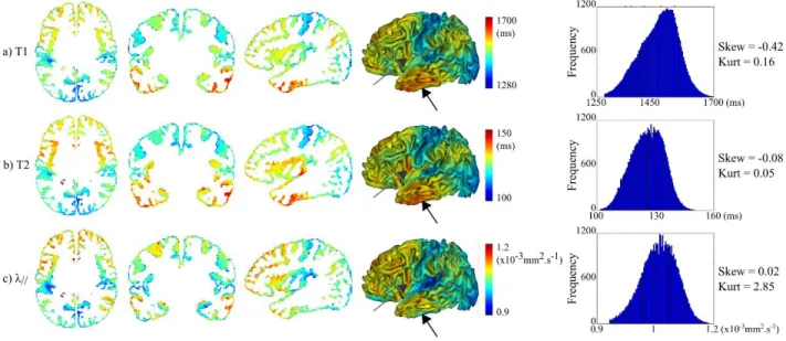
These spatial differences were better highlighted at the group level, based on averaged parametric maps over all infants (Figure 4). Although we did not take into account that parameters also vary across regions at the mature stage in the adult brain, these individual and group results suggested an asynchrony of maturation across cortical regions, with advanced maturation of primary cortices compared with associative cortices. Nevertheless, we could not disentangle which parameter better described the maturation process, since each of T1, T2 and λ// maps provided slightly different information. The global distribution
of mature vs immature cortical regions was equivalent in the three maps, but some substantial mismatches were observed locally (see arrows in Figure 4). For instance, the inferior temporal region showed high T1 and T2 values but intermediate λ// values. Similarly,
16/38
observation was rather consistent with a recent high-resolution mapping of the adult brain, highlighting that the temporal region has specific properties, with low myelin content but low values of mean diffusivity (Fukutomi et al., 2018). As a whole, our results might suggest that T1 mainly reflects the myelin content whereas axial diffusivity rather provides microstructural information on neuronal cytoarchitecture.
Also, note that the distribution of parametric values differed in some aspects (right column in Figure 4). For instance, while the T2 and λ// distributions were quite symmetrical (with
absolute values of skewness measure very close to zero), the T1 distribution was clearly left-skewed (with a higher proportion of long than short T1 values, skewness = -0.42). On the other hand, the λ// distribution looked like to a normal distribution, whereas the T1 and T2
distributions were rather platykurtic (meaning that extreme values were less frequent). Altogether, these observations suggested that these quantitative parameters provide different information on cortical microstructure although the overall trend across regions is rather similar.
Figure 4: Average maps of quantitative parameters over the infants group. For T1 (a), T2 (b) and λ// (c) parameters, average 2D maps were computed within the cortical ribbon and over
the 17 infants after the DISCO+DARTEL registration. They were further projected in 3D on the left cortical surface of a 6w-old infant. The distribution of parametric values over these maps is plotted on the right column, highlighting that each modality shows a different distribution. Gray arrows point out some substantial mismatches across parametric maps (temporal and precentral regions respectively).
17/38 3.2 Clustering analysis of cortical maturation
3.2.1 GMM settings
We performed clustering analyses with the GMM algorithm considering all voxels of the cortical ribbons for the 17 infants altogether, and we tested different settings. Considering the {T1-T2-λ//} combination as input data, Silhouette coefficients suggested that the
“spherical” model outperformed other models regardless of the number of clusters (it showed higher mean value and lower standard deviation across different experiments; Figure 5a). Fixing this model as covariance matrix, we further evaluated the effect of the parameter combination. Silhouette coefficients were the highest for single parameters {λ//},
{T1}, {T2}, followed successively by combinations of 2 parameters {T1- λ//} and {T1-T2}, then
{T2- λ//}, and finally the combination of 3 parameters {T1-T2-λ//} (Figure 5b). Nevertheless,
when we computed the normalized volumes to evaluate the cluster balance (Figure 5c), we observed that analyses of single parameters, as well as the combinations {T2- λ//} and
{T1-T2}, provided clusters with higher volume variability than the combinations {T1- λ//} and
{T1-T2-λ//}, meaning that one cluster was over represented compared to others for some
infants. As a whole, the input combination {T1- λ//} showed good Silhouette coefficient and
low variability in the cluster normalized volumes. To further analyze the potential of this combination, we tested different weightings attributed to T1 and λ//. The weighted
combination {T1- ¼ λ//} appeared as the best compromise based on a similar reasoning with
Silhouette coefficients and variability in the cluster volumes (Supplementary Figure 2). Figure 5: Selection of GMM settings. Silhouette coefficients were computed for a) different covariance matrices (considering the {T1-T2-λ//} combination as input, and 3 to 10 clusters)
and b) different input combinations (considering the “spherical” model as covariance matrix, and 3 to 10 clusters). Dotted lines represent mean values of each series. c) Standard deviations (SD) of the clusters normalized volumes (Vn) were also computed for the latter settings.
18/38
Once the model setting and the combination were fixed, we evaluated the impact of the number of clusters (Supplementary Figure 3). Based on Silhouette coefficients, we first observed that the setting with 4 clusters was not reliable as it led to obvious voxel mislabeling (one cluster showed a high proportion of negative Silhouette coefficients). Besides, no relevant information was added when considering 6 or more clusters (in those cases, at least one cluster was under represented in terms of volume, with less than 2% of the total volume). For the two remaining numbers of clusters, we compared the cluster balance (i.e. the variability in the cluster normalized volumes) according to the infants’ age (Supplementary Figure 3b), and we finally selected the analysis with 5 rather than 3 clusters, as it provided clusters with more homogeneous volumes across all infants.
3.2.2 Differences in microstructure and asynchrony of maturation across cortical regions
Once the clusters were identified based on the previous optimal settings (spherical model, combination {T1- ¼ λ//}, 5 clusters), we labeled them in terms of microstructural properties,
with the assumption that both T1 and λ// parameters should decrease with the tissue
myelination and the cytoarchitectural complexity. When T1 and λ// values were averaged
over each cluster for each infant (Figure 6a-b), the inter-cluster separation was clear (particularly for T1), and the intra-cluster homogeneity was good, leading to an easy ordering of the clusters in terms of microstructural stages (1 to 5). To interpret these stages in terms
19/38
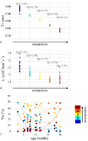
of maturation, we further measured age-related changes in the normalized volumes of clusters (Figure 6c). We showed that, over the 5 clusters, the first two had immature patterns (age-related decreases), the last two had mature patterns (age-related increases), and the middle one had an intermediate pattern (inverse U-shape). This suggested that this clustering based on microstructural properties could be interpreted in terms of maturation over the infants group.
Figure 6: Characterization of the 5 clusters properties for the combination {T1- ¼ λ//}. The
average of T1 (a) and λ// (b) parameters over each individual cluster (1 point by infant)
enabled us to order the clusters in terms of microstructural stages (decreasing values). Quartile coefficients of dispersion (Qc) suggested a good intra-cluster homogeneity. c) Normalized volumes (%) were computed for each cluster as a function of the infants’ age (in weeks, dotted lines represent a 3-order polynomial fit for each cluster), linking microstructural and maturational stages.
The spatial distribution of the 5 clusters clearly illustrated maturation differences across cortical regions in each infant, and also age-related progression across infants (Figure 7 and Supplementary Figure 4 for the 2D maps). Basically, primary sensorimotor regions were the most mature regions in all infants, around the calcarine fissure in primary visual cortex V1 [1], Heschl gyrus in primary auditory cortex A1 [2], around the central sulcus in primary somatosensory cortex S1 [3] and primary motor cortex M1 [4]. Surrounding regions such as
20/38
the internal occipital region [5] or the planum temporale [6] also seemed to mature early on. In some infants, a temporo-occipital region that might correspond to the motion-related MT area appeared as relatively mature [7]. In some of the oldest infants, the superior parietal lobule [8] reached a high maturation level, at least higher than the close supramarginal and angular regions [9]. In almost all infants, associative regions such as the superior temporal gyrus [10] or the inferior frontal region [11] were immature in comparison with previous regions, the least mature being the middle pre-frontal [12], and the superior frontal [13] regions. On the ventral part of the brain, the fusiform region [14] seemed to have an intermediate maturation, in-between the advanced maturation of occipital and parahippocampic regions and the delayed maturation of the inferior temporal lobe and pole. On the medial surface, the middle part of the cingulate gyrus [15] seemed to mature before its anterior part [16].
Although all these observations concerned most of the infants and were relatively coherent spatially over the developmental period, we observed some inter-individual variability that was not related to age. Indeed, spatial patterns of the cluster distribution varied across infants of similar ages. Note for instance in Figure 7 that 2 infants (highlighted in red) might have an advanced maturation, whereas 2 infants (highlighted in blue) might have a delayed maturation. This suggested that each infant brain might follow its own maturation trajectory. Although the small group size prevented us to statistically assess the influence of different subject factors, inter-individual variability in cortical maturation did not seem to be related to sex and gestational age at birth, but might partially relate to other morphometric parameters of brain growth and cortical folding (see Supplementary Figure 1).
Figure 7: 3D individual distributions of the 5 maturational clusters for all infants. The majority labels were measured over a cylinder perpendicular to individual cortical surfaces (inflated surfaces are here shown for visualization purposes). Left (a, c) and right (b, d) maps are shown with lateral (a, b) and medial (c, d) views. Note that the clusters numbering is the same across infants. Some anatomical regions are outlined: 1) primary visual cortex V1 around the calcarine fissure, 2) primary auditory cortex A1 in the Heschl gyrus, 3) primary somatosensory cortex S1 around the central sulcus, 4) primary motor cortex M1, 5) internal occipital region, 6) planum temporal region, 7) motion-related of the middle temporal area, 8) superior parietal gyrus, 9) supramarginal and angular regions, 10) superior temporal gyrus, 11) inferior frontal gyrus, 12) middle pre-frontal gyrus, 13) superior pre-frontal gyrus, 14) fusiform gyrus, 15) middle part of the cingulate gyrus, 16) anterior part of the cingulate gyrus. Doted red (resp. blue) boxes highlight infants that might have an advanced (resp. delayed) maturation compared to infants of similar age.
22/38
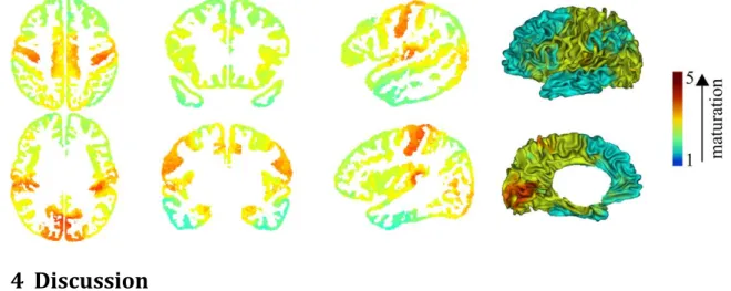
Finally, the average map of the cluster spatial distribution, computed over the infants group after the DISCO+DARTEL registration, summarized these patterns of maturation (Figure 8). These representations are rather similar to the illustrations provided by Pr Flechsig about a century ago (Flechsig, 1920), displaying the maturation ordering of cortical regions based on
post mortem myelin staining of sub-cortical white matter.
Figure 8: Average clustering map over the infants group. Average 2D map was computed within the cortical ribbon and over the 17 infants after the DISCO+DARTEL registration. For visualization purposes, it was projected in 3D on the left cortical surface of a 6w-old infant.
4 Discussion
In this study, we mapped the cortical microstructure with in vivo MRI in infants between 1 and 5 months of age. This topic has not been much addressed so far compared with the largely studied maturation of the white matter (see (Dubois et al., 2014a) for a review), due to constraints inherent to the cortex immaturity and morphology (small thickness but complex folding patterns). We analyzed multiple parameters over the whole cortex, which enabled us to identify clusters with different microstructural properties, and to characterize the temporal profiles and spatial patterns of maturation across cortical regions both at the intra-individual and group levels.
4.1 Mapping the cortical maturation in infants with MRI: methodological considerations on univariate and multi-parametric approaches
So far, only a few studies have evaluated the cortical microstructure in the newborn and infant brain. Here, we used quantitative parameters that could be reliably compared across brain regions and across subjects without requiring spatial bias correction or signal normalization as it might be the case for T1w (Travis et al., 2014; Westlye et al., 2010) and T2w (Leroy et al., 2011a) intensity, or T1w/T2w ratio (Grydeland et al., 2013). Contrarily to derived parameters (e.g. myelin water fraction (Deoni et al., 2015), magnetic susceptibility (W. Li et al., 2014)), we focused on direct parameters that could be quantified in a short acquisition time: T1 (Deoni et al., 2015; Friedrichs-Maeder et al., 2017) and T2 relaxation
23/38
times, and DTI axial diffusivity //. This latter parameter was preferred to DTI anisotropy
(Ball et al., 2013; McKinstry et al., 2002) or mean diffusivity (Grydeland et al., 2013; Friedrichs-Maeder et al., 2017) because it provided the best contrast between grey and white matter, and it could be specifically measured within the cortical ribbon, which displays minimal // values regardless of the maturational stage. The plausible microstructural
significance of those parameters is discussed below in Section 4.2. Besides, whereas all previous studies were based on single parameters, we performed multi-parametric analyses in addition to univariate ones.
To keep the acquisition time reasonable for spontaneously asleep infants, we used dedicated EPI sequences to acquire parametric maps (Poupon et al., 2010). A posteriori corrections of geometric distortions were thus required to measure those parameters within the cortical ribbon in a reliable way with anatomical T2w images as reference. T1 maps showed the highest distortions probably because the related sequence did not use parallel imaging. Our post-processing approach based on linear and non-linear registrations was successful to correct local distortions in all parametric maps, leading to residual distances below the spatial resolution of anatomical images. Although these results were satisfactory, alternative approaches based on readout-segmented EPI (Porter and Heidemann, 2009) or field maps (Jezzard, 2012) might be considered in the future to deal with such distortions.
To reliably analyze the cortical microstructure, the next issue was to identify the cortical ribbon precisely on each parametric map and for each infant. This was particularly challenging given the small cortical thickness (expected to be less than 2mm in some regions) (Geng et al., 2017; Li et al., 2015; Lyall et al., 2015; Meng et al., 2017) and the spatial resolution of T1, T2 and // maps (1.8mm isotropic). Since we aimed not to miss cortical voxels due to
residual local errors of registration, we used a semi-automatic procedure based on anatomical images and FA maps. While it was rather robust to exclude CSF voxels, the resulting cortical ribbon might have included some voxels of sub-cortical white matter. Nevertheless, we checked visually that the proportion of those voxels was small compared with the proportion of cortical voxels. Furthermore, adjacent tissues of cortex and white matter are expected to show related maturational patterns. Indeed, Flechsig’s maps on sub-cortical white matter myelination are often interpreted in terms of sub-cortical maturation. A recent study based on the myelin water fraction also showed strong correlations between cortical and white matter values (in 63 of 66 identified regions (Croteau-Chonka et al., 2016)). Another study reported that the grey matter regions and the underlying WM connections have inter-related advancement of maturation (Friedrichs-Maeder et al., 2017). This suggests that inevitable small contamination by WM values in our study would not significantly change our results and interpretation of cortical maturation.
To visualize single parameters on 3D cortical surfaces, we measured local values over a small cylinder screening the inner surface and intersecting the cortical ribbon, as proposed in a
24/38
previous study (Leroy et al, J. Neuroscience 2011). We did not consider the middle surface of the cortex as often done in adults and children studies because of the small cortical thickness in infants with variability across regions (Geng et al., 2017; Li et al., 2015; Lyall et al., 2015; Meng et al., 2017), the limited spatial resolution of parametric maps (1.8mm) and anatomical T2w images (1mm), and the residual spatial mismatches between the cortical segmentation and quantitative measures. Over the local cylinder, we computed either minimal values for //, or mean values for T1 and T2. The // approach might be more specific of cortical
maturation than those based on T1 and T2, which might be slightly influenced by a small proportion of sub-cortical white matter voxels. Nevertheless, we expected the possible bias to be small, to the extent that both tissues are supposed to mature in a synchronous and coherent way.
For all parameters, the whole-brain progression of cortical maturation across infants was observed as a global decrease with age. However, the differential microstructure across cortical regions (discussed below in Section 4.3) was much more visible over the infant group than at the individual level. In addition, we observed differences in the distribution of T1, T2 and // values over the whole cortex and over the group, suggesting that each parameter
differently reflects the cortical microstructure. Besides, the clustering approach benefitted from the complementarity of MRI parameters. While it was performed on volumes, the 3D visualization of the results on cortical surfaces was based on the identification of cluster majority labels. Although we did not take into account the parameters variability across regions at the mature stage in the adult brain (Fukutomi et al., 2018; Glasser et al., 2014; Sereno et al., 2013), we interpreted our findings in infants in terms of maturation as we observed age-related variations in each parameter and in each cluster volume. As a whole, this study enabled us to highlight the local maturation of cortical voxels, and to show the differential progression across cortical regions at both the individual and group levels. These successive observations supported the potential of a multi-parametric approach against univariate approaches.
Its technical implementation consisted of a clustering analysis with a GMM algorithm using a k-means initialization and an Expectation-Maximization iterative process. While other clustering algorithms (e.g. k-means) might be tested in future studies, we chose the GMM algorithm because it is the main generative clustering model, making the testing of clustering quality and generalizability easier. Here, the covariance matrix model, the input data combination, and the number of clusters were selected sequentially using the Silhouette coefficient as a discriminant index, and the variability in the cluster volumes as a marker of under- or over-representation. Experiments showed that the clustering performances were optimized with the {T1- ¼ λ//} combination. This supported the multi-parametric approach
25/38
(Kulikova et al., 2015). Nevertheless, if only a single MRI parameter can be acquired, T1 mapping might be preferred rather than DTI and T2, to assess the cortical maturation. With regard to the clustering analysis, selecting the optimal number of clusters might be problematic as it might influence the correct interpretation of results. Here we observed that the variability in cortical T1 and λ// parameters over this infant group was accurately
characterized based on 5 clusters which showed three distinct patterns of microstructure and maturation: either immature (age-related decreases for 2 clusters), mature (age-related increases for 2 clusters), or intermediate (inverse U-shape for 1 cluster). These three patterns might still be detected with the 3-cluster setting, whereas their reliable distribution into 4 clusters might be problematic, perhaps resulting in the misclassification issue that we observed with this middle number. As a whole, we cannot exclude that different numbers of clusters might be relevant when considering other or broader developmental periods than early infancy.
4.2 Microstructural and morphological correlates of cortical maturation
Once methodological aspects were fixed, we identified 5 clusters of cortical voxels over the whole infant group, independently of both the infants’ age and the voxel localization, and we labeled them in terms of maturational stage. The clustering implementation implied that these clusters were characterized by distinct T1 and λ//. After averaging these parameters
over each cluster and for each infant, we considered that the cluster maturational stage increased when T1 and λ// values decreased, given the expected maturation-related changes
in these parameters. We further observed that the clusters normalized volumes varied over this developmental period, coherently with the labelling of maturational stages (i.e. the proportion of immature clusters decreased with the infants’ age, and vice versa for mature regions).
MRI parameters are known to relate to several microstructural properties of the adult cortex, such as the neural, glial and fiber density, the intra-cortical myelination, the layers proportions, the columnar properties, and others. In the infant cortex, they also provide distinct and complementary information on both the maturation and microstructure. T1 mainly provides information on the myelin content, as suggested in adults (Lutti et al., 2014; Sereno et al., 2013). Axial diffusivity λ// might rather provide microstructural information on
neuronal cytoarchitecture and reflect the intense development of both dendritic arborization and synaptogenesis during infancy (Huttenlocher and Dabholkar, 1997), in the continuity of observations during the preterm period (Ball et al., 2013; McKinstry et al., 2002). These regional properties might be consistent throughout development, as our specific measures in the inferior temporal region (high T1 and T2 values but intermediate λ// values) agreed
with a recent mapping of the adult brain (Fukutomi et al., 2018). Nevertheless, similarly to previous studies of white matter bundles (Dubois et al., 2014a; Kulikova et al., 2015), further
26/38
work is required in order to relate our results with the adult regions variability, and to test the hypothesis that regions with the highest myelination (Glasser et al., 2014) or the most complex microstructure (Fukutomi et al., 2018) at the mature stage are the first to mature and to display such properties throughout development (Flechsig, 1920). In our study, T2 appeared less informative than T1 and λ// to characterize cortical differences over infants,
either because T2 relies on the same mechanisms as T1 and λ//, or because the other
determinants of T2 signal (e.g. iron content) do not change intensively over this age range. Although all parameters probably fluctuate radially within the cortical ribbon, it was not possible to distinguish cortical layers given the spatial resolution of parametric maps. In the future, imaging approaches at ultra-high field (e.g. 7T) might provide the mapping of finer-grained features in the developing brain.
In parallel to microstructural changes, the cortex also demonstrates intense growth and morphological development throughout infancy. The cortical volume increases mainly because of surface expansion (Gilmore et al., 2007, 2011; Hill et al., 2010; Knickmeyer et al., 2008; Li et al., 2013; Makropoulos et al., 2016), in relation with the increasing folding complexity (Dubois et al., 2018; Kim et al., 2016; G. Li et al., 2014). Cortical thickness also consistently increases during the first post-natal year (Geng et al., 2017; Li et al., 2015; Lyall et al., 2015; Meng et al., 2017), with different patterns of growth than the cortical folding (Nie et al., 2014). We might thus wonder to what extent these morphological changes affect our microstructural observations. A previous study in children between 1 and 6 years old showed that the cortical maturation (measured with the myelin water fraction) is negatively correlated to cortical thickness in 16 of 66 identified regions (Croteau-Chonka et al., 2016). Given the spatial resolution of parametric maps (1.8mm isotropic), we cannot exclude that partial volume effects between cortex and white matter exist within the identified cortical ribbon. Some variations might further exist across regions, with a higher WM contamination in thinner than thicker cortices. Unfortunately, we could not address this issue practically since a reliable estimation of cortical thickness is highly challenging in infants given its low values (Geng et al., 2017; G. Li et al., 2014; Lyall et al., 2015; Meng et al., 2017) and because of the tissue contrast inversion on anatomical MRI (Walhovd et al., 2017). Besides, based on visual observations, our univariate and multi-parametric results did not seem to be related to the cortical surface curvature or to the folding patterns. This convinced us about the reliability of our approach while we were surprised by previous T1 observations highlighting a mismatch in maturation between the main sulci and surrounding regions (Deoni et al., 2015). In brief, while the identified cortical clusters relied on complementary microstructural maturation mechanisms (intra-cortical myelination, neuronal differentiation, dendritic arborization and synaptic growth…), they seemed to be weakly affected by the macroscopic changes related to cortical morphology throughout infancy.
27/38 4.3 Mapping the spatial progression of cortical maturation throughout infancy with
multi-parametric MRI
Our original clustering approach allowed us to observe differences across cortical regions both at the individual and group levels, with maturation proceeding first in primary sensori-motor areas, then in adjacent unimodal associative cortices, and finally in higher-order associative regions. This pattern of progression strongly agreed with benchmark post
mortem studies (Brody et al., 1987; Flechsig, 1920; Kinney et al., 1988) which showed high
variability in fiber myelination within and across fiber systems, with a few discrepancies in some regions (e.g. in the frontal and temporal lobes). In fact, the time-related sequence of myelination mechanisms (i.e. the onset, the rate, the interval of progression) differs across functional regions during the first two post-natal years (Brody et al., 1987; Kinney et al., 1988), and including all these relevant factors is required to highlight complex myelination patterns. Considering complementary MRI parameters measured at different ages might be a first step in this direction. The maturational clusters that we observed were also consistent with patterns of cortical synaptogenesis (Huttenlocher and Dabholkar, 1997) and with regional variations of the basilar dendritic complexity of lamina V pyramidal neurons showing that the developmental time course from birth to adulthood is more protracted for supramodal (BA10) than for primary or unimodal cortical areas (BA4, BA3-1-2, BA18) (Travis et al., 2005). In addition to major regional differences, we could also show local discontinuities for specific regions such as the MT area for some infants.
Apart from these regional differences observed both in each infant and over the group, we highlighted substantial inter-individual variability in the maturational patterns. Although the cortical maturation mainly depends on age, some infants showed delayed or advanced brain maturation in comparison with other babies of similar ages. We suspected that these differences might be partially related to global inter-individual variability in brain growth and development, independently of sex or gestational age at birth. In particular, complex patterns of maturation across functional regions (Brody et al., 1987; Kinney et al., 1988) interacting with the variable behavioral acquisitions might contribute to these differences across infants. Nevertheless we cannot exclude that an incorrect estimation of the conception day (and so of the gestational length) might be responsible for part of these discrepancies. While our results suggested the potential of studying the cortical maturation in vivo, we could not validate them quantitatively since benchmarks on the whole brain maturation are still lacking in infants over this developmental period. This first study should thus be confirmed by future studies on other cohorts, notably with longitudinal imaging of infants over the first post-natal year. One interesting aspect to be tested would be whether the progression of cortical maturation is related to the growth in cortical surface throughout infancy (Hill et al., 2010). In fact, we might expect that the cortex at birth is less mature in high-expansion
28/38
regions than in low-expansion regions since the cortical growth is related to dendritic arborization and myelination that spread the cortical columns.
5 Conclusion
In this study, we characterized the differential microstructure and the asynchronous maturation of cortical regions in vivo, using multi-parametric MRI (T1, T2 and λ//) in infants
over the first post-natal months. The main contributions relied on 1) the whole-brain analysis opposed to a priori spatially localized regions, and 2) the clustering of complementary parameters that are impacted by different maturational mechanisms such as intra-cortical myelination and dendritic arborization. In future studies, this approach might be extended to other developmental periods, and it might complement previous approaches uniquely based on cortical thickness. It also seems appropriate to evaluate the in vivo relationship between cortical maturation and the development of functional systems and behavioral capacities throughout infancy, as recent studies in children postulated microstructural bases of cognitive performances such as face recognition (Gomez et al., 2017).
6 Supplementary Figures
Supplementary Figure 1: Infants’ characteristics. a) Post-natal ages are represented as a function of maturational ages (= gestational age at birth + post-natal age, corrected for a reference gestational period of 41 weeks). The dotted black line shows the identity function. Boys and girls are symbolized by crosses and circles respectively. Averaged hemispheric brain volume (b), cortical surface (c) and sulcation index (d) are plotted as a function of infants’ age as described in (Dubois et al., 2018). Dotted black lines represent linear fits for each measure. Red (resp. blue) marks highlight infants that might have an advanced (resp. delayed) cortical maturation according to the clustering results illustrated in Figure 7.
29/38
Supplementary Figure 2: Selection of T1 and λ// weightings for the clustering analysis. a)
Silhouette coefficients were computed for different T1 and λ// weighted inputs (considering
3 to 10 clusters). Dotted lines represent mean values of each series. b) Standard deviations (SD) of the clusters normalized volumes (Vn) were also computed for these different weighted inputs. Similarly to the reasoning related to Figure 5, the combination {T1- ¼ λ//}
appeared as the most relevant across the different cluster numbers, as it showed on average the highest Silhouette coefficient and the lowest volume variability across clusters.
30/38
Supplementary Figure 3: Selection of the number of clusters for the optimized setting with “spherical” model as covariance matrix, and the weighted combination {T1- ¼λ//}
(optimization resulting from Figure 5 and Supplementary Figure 2). a) Silhouette coefficients (s) are plotted for various numbers of clusters. Blue dotted lines represent the average Silhouette coefficients. For the setting with 4 clusters, the black ellipsoid outlines a cluster with a high proportion of negative Silhouette coefficients meaning that many voxels of this cluster (63%) were mislabeled. For settings with 6 clusters or more, black asterisks highlight clusters representing less than 2% of the total volume. According to these plots, only settings with 3 and 5 clusters seemed to be relevant. b) Standard deviations (SD) of the clusters normalized volumes (Vn) are shown as a function of the infants’ age for 3 and 5 clusters. The variability is lower for this latter number, suggesting its higher relevance.
31/38
Supplementary Figure 4: 2D individual maps for the 5 clusters of maturation. The maturational differences across cortical regions are clearly visible in each infant, as well as the age-related progression across infants observed in 3D (Figure 7 and 8).