HAL Id: inria-00000156
https://hal.inria.fr/inria-00000156v3
Submitted on 9 Nov 2005
HAL is a multi-disciplinary open access
archive for the deposit and dissemination of
sci-entific research documents, whether they are
pub-lished or not. The documents may come from
teaching and research institutions in France or
abroad, or from public or private research centers.
L’archive ouverte pluridisciplinaire HAL, est
destinée au dépôt et à la diffusion de documents
scientifiques de niveau recherche, publiés ou non,
émanant des établissements d’enseignement et de
recherche français ou étrangers, des laboratoires
publics ou privés.
Understanding BitTorrent: An Experimental
Perspective
Arnaud Legout, Guillaume Urvoy-Keller, Pietro Michiardi
To cite this version:
Arnaud Legout, Guillaume Urvoy-Keller, Pietro Michiardi. Understanding BitTorrent: An
Experi-mental Perspective. [Technical Report] 2005, pp.16. �inria-00000156v3�
Understanding BitTorrent: An Experimental
Perspective
Arnaud Legout
I.N.R.I.A.
Sophia Antipolis, France
Email: [email protected]
Guillaume Urvoy-Keller and Pietro Michiardi
Institut Eurecom
Sophia Antipolis, France
Email: {Guillaume.Urvoy,Pietro.Michiardi}@eurecom.fr
Technical Report
Abstract— BitTorrent is a recent, yet successful peer-to-peerprotocol focused on efficient content delivery. To gain a better understanding of the key algorithms of the protocol, we have instrumented a client and run experiments on a large number of real torrents. Our experimental evaluation is peer oriented, instead of tracker oriented, which allows us to get detailed information on all exchanged messages and protocol events. In particular, we have explored the properties of the two key algorithms of BitTorrent: the choke and the rarest first algorithms. We have shown that they both perform remarkably well, but that the old version of the choke algorithm, that is still widely deployed, suffers from several problems. We have also explored the dynamics of a peer set that captures most of the torrent variability and provides important insights for the design of realistic models of BitTorrent. Finally, we have evaluated the protocol overhead. We have found in our experiments a small protocol overhead and explain under which conditions it can increase.
I. INTRODUCTION
In few years, peer-to-peer applications have become among the most popular applications in the Internet [1], [2]. This success comes from two major properties of these applica-tions: any client can become a server without any complex configuration, and any client can search and download contents hosted by any other client. These applications are based on specific peer-to-peer networks, e.g., eDonkey2K, Gnutella, and FastTrack to name few. All these networks focus on content localization. This problem has raised a lot of attention in the last years [3]–[6].
Recent measurement studies [1], [2], [7], [8] have reported that peer-to-peer traffic represents a significant portion of the Internet traffic ranging from 10% up to 80% of the traffic on backbone links depending on the measurement methodology and on their geographic localization. To the best of our knowledge, all measurements studies on peer-to-peer traffic consider traces from backbone links. However, it is likely that peer-to-peer traffic represents only a small fraction of the traffic on enterprises networks. The main reason is the lack of legal contents to share and the lack of applications in an enterprise context. This is why network administrators filter out the peer-to-peer ports in order to prevent such traffic on
their network. However, we envision at short or mid term a widespread deployment of peer-to-peer applications in enter-prises. Several critical applications for an enterprise require an efficient file distribution system: OS software updates, antivirus updates, Web site mirroring, backup system, etc. As a consequence, efficient content delivery will become an important requirement that will drive the design of peer-to-peer applications.
BitTorrent [9] is a new peer-to-peer application that has became very popular [1], [2], [7]. It is fundamentally different from all previous peer-to-peer applications. Indeed, BitTorrent does not rely on a peer-to-peer network federating users sharing many contents. Instead, BitTorrent creates a new peer-to-peer transfer session, called a torrent, for each content. The drawback of this design is the lack of content localization support. The major advantage is the focus on efficient content delivery.
In this paper, we perform an experimental evaluation of the key algorithms of BitTorrent. Our intent is to gain a better understanding of these algorithms in a real environment, and to understand the dynamics of peers. Specifically, we focus on the client local vision of the torrent. We have instrumented a client and run several experiments on a large number of torrents. We have chosen torrents with different characteristics, but we do not pretend to have reach completeness. Instead, we have only scratched the surface of the problem of efficient peer-to-peer content delivery, yet we hope to have done a step toward a better understanding of efficient delivery of data in peer-to-peer.
We took during this work several decisions that restrict the scope of this study. We have chosen to focus on the behavior of a single client in a real torrent. While it may be argued that a larger number of peers instrumented would have given a better understanding of the torrents, we took the decision to be as unobtrusive as possible. Increasing the number of instrumented clients would have required to either control those clients ourselves, or to ask some peers to use our instrumented client. In both cases, the choice of the instrumented peer set would have been biased, and the behavior of the torrent impacted. On the contrary, our decision was to understand how a new
peer (our instrumented peer) joining a real torrent will behave. A second decision was to evaluate only real torrents. In such a context it is not possible to reproduce an experiment, and thus to gain statistical information. However, studying the dynamic of the protocol is as important as studying its statistical properties. Also, as we considered a large number of torrents and observed a consistent behavior on these tor-rents, we believe our observations to be representative of the BitTorrent protocol.
Finally, we decided to present an extensive trace analysis, rather than a discussion on the possible optimizations of the protocol. Studying how the various parameters of BitTorrent can be adjusted to improve the overall efficiency, and propos-ing improvements to the protocol only makes sense if deficien-cies of the protocol or significant room for improvements are identified. We decided in this study to make the step before, i.e., to explore how BitTorrent is behaving on real torrents. We found in particular that the last piece problem, which is one of the most studied problem with proposed improvements of BitTorrent is in fact a marginal problem that cannot be observed in our torrent set. It appears to us that this study is a mandatory step toward improvements of the protocol, and that it is beyond the scope of our study to make an additional improvement step.
To the best of our knowledge this study is the first one to offer an experimental evaluation of the key algorithms of BitTorrent on real torrents. In this paper, we provide a sketch of answer to the following questions:
• Does the algorithm used to balance upload and download rate at a small time scale (called the choke algorithm, see section II-C.1) provide a reasonable reciprocation at the scale of a download? How does this algorithm behave with free riders? What is the behavior of the algorithm when the peer is both a source and a receiver (i.e., a leecher), and when the peer is a source only (i.e., a seed)?
• Does the content pieces selection algorithm (called rarest first algorithm, see section II-C.2) provide a good entropy of the pieces in the torrent? Does this algorithm solve the last pieces problem?
• How does the set of neighbors of a peer (called a peer set) evolve with time? What is the dynamics of the set of peers actively transmitting data (called active peer set)?
• What is the protocol overhead?
We present the terminology used throughout this paper in section II-A. Then, we give a short overview of the BitTorrent protocol in section II-B, and we give a detailed description of its key algorithms in section II-C. We present our ex-perimentation methodology in section III, and our detailed results in section IV. Related work is discussed in section V. We conclude the paper with a discussion of the results in section VI.
II. BACKGROUND
A. Terminology
The terminology used in the peer-to-peer community and in particular in the BitTorrent community is not standardized.
For the sake of clarity, we define in this section the terms used throughout this paper.
Files transfered using BitTorrent are split in pieces, and each piece is split in blocks. Blocks are the transmission unit on the network, but the protocol only accounts for transfered pieces. In particular, partially received pieces cannot be served by a peer, only complete pieces can.
Each peer maintains a list of other peers it can potentially send pieces to. We call this list the peer set. This notion of peer set is also known as neighbor set. We call local peer, the peer with the instrumented BitTorrent client, and remote
peers, the peers that are in the peer set of the local peer.
We say that peer A is interested in peer B when peer B has pieces that peer A does not have. Conversely, peer A is not
interested in peer B when peer B has a subset of the pieces
of peer A. We say that peer A chokes peer B when peer A cannot send data to peer B. Conversely, peer A unchokes peer
B when peer A can send data to peer B.
A peer can only send data to a subset of its peer set. We call this subset the active peer set. The choke algorithm (described in section II-C.1) is in charge of determining the peers being part of the active peer set, i.e., which remote peers will be choked and unchoked. Only peers that are unchoked by the local peer and interested in the local peer are part of the active peer set.
A peer has two states: the leecher state, when it is down-loading a content, but does not have yet all pieces; the seed
state when the peer has all the pieces of the content. For short,
we can say that a peer is a leecher when it is in leecher state and a seed when it is in seed state.
B. BitTorrent Overview
BitTorrent is a P2P application that capitalizes on the bandwidth of peers to efficiently replicate contents on large sets of peers. A specificity of BitTorrent is the notion of
torrent, which defines a session of transfer of a single content
to a set of peers. Each torrent is independent. In particular, there is no reward or penalty to participate in a given torrent to join a new one. A torrent is alive as long as there is at least one seed in the torrent. Peers involved in a torrent cooperate to replicate the file among each other using swarming techniques. In particular, the file is split in pieces of typically 256 kB, and each piece is split in blocks of 16 kB. Other piece sizes are possible.
A user joins an existing torrent by downloading a
.tor-rent file usually from a Web server, which contains
meta-information on the file to be downloaded, e.g., the number of pieces and the SHA-1 hash values of each piece, and the IP address of the so-called tracker of the torrent. The tracker is the only centralized component of BitTorrent, but it is not involved in the actual distribution of the file. It only keeps track of the peers currently involved in the torrent and collects statistics on the torrent.
When joining a torrent, a new peer asks to the tracker a list of IP addresses of peers to connect to and cooperate with, typically 50 peers chosen at random in the list of peers currently involved in the torrent. This set of peers
forms the peer set of the new peer. This peer set will be augmented by peers connecting directly to this new peer. Such peers are aware of the new peer by receiving its IP address after a request to the tracker. Each peer reports its state to the tracker every 30 minutes in steady-state regime, or when disconnecting from the torrent, indicating each time the amount of bytes it has uploaded and downloaded since it joined the torrent. A torrent can thus be viewed as a collection of interconnected peer sets. If ever the number of peers in the peer set of the new peer falls below a predefined threshold (typically 20 peers), this peer will contact the tracker again to obtain a new list of IP addresses of peers. By default, the maximum peer set size is 80. Moreover, a peer should not exceed a threshold of 40 initiated connections among the 80 at each time. As a consequence, the 40 remaining connections should be initiated by remote peers. This policy guarantees a good interconnection among the peer sets in the torrent and avoid the creation of cliques.
Each peer knows which pieces each peer in its peer set has. The consistency of this information is guaranteed by the exchange of messages described in section IV-D. The exchange of pieces among peers is governed by two core algorithms: the choke and the rarest first algorithms. Those algorithms are further detailed in section II-C.
C. BitTorrent Algorithms Description
We focus here on the two most important algorithms of BitTorrent: the choke algorithm and the rarest first piece selection algorithm. We will not give all the details of these algorithms, but we will explain the main ideas behind them.
1) Choke Algorithm: The choke algorithm was introduced
to guarantee a reasonable level of upload and download reciprocation. As a consequence, free riders, i.e., peers that never upload, should be penalized. The choke algorithm makes an important distinction between the leecher state and the seed state. This distinction is very recent in the BitTorrent protocol and appeared in version 4.0.0 of the mainline client [10]. We are not aware of a documentation of this new algorithm and of an implementation of it apart from the mainline client. In the following, we describe the algorithm with the default parameters. By changing the default parameters it is possible to increase the size of the active peer set and the number of optimistic unchokes.
In this section, interested always means interested in the local peer, and choked always means choked by the remote peer.
When in leecher state, the choke algorithm is called every ten seconds and each time a peer leaves the peer set, or each time an unchoked peer becomes interested or not interested. As a consequence, the choke period can be much shorter than 10 seconds. Each time the choke algorithm is called, we say that a new round starts, and the following steps are executed. 1) At the beginning of every three rounds, i.e., every 30 seconds, the algorithm chooses one peer at random that is choked and interested. We call this peer the planned optimistic unchoked peer.
2) The algorithm orders peers that are interested and have sent at least one block in the last 30 seconds according to their download rate (to the local peer). A peer that has not sent any block in the last 30 seconds is called snubbed. Snubbed peers are excluded in order to guarantee that only active peers are unchoked.
3) The three fastest peers are unchoked.
4) If the planned optimistic unchoked peer is not part of the three fastest peers, it is unchoked and the round is completed.
5) If the planned optimistic unchoked peer is part of the three fastest peers, another planned optimistic unchoked peer is chosen at random.
a) If this peer is interested, it is unchoked and the round is completed.
b) If this peer is not interested, it is unchoked and a new planned optimistic unchoked peer is chosen at random. Step 5a is repeated with the new planned optimistic unchoked peer. As a consequence, more than 4 peers can be unchoked by the algorithm. However, only 4 interested peers can be unchoked in the same round. Unchoking not interested peers allows to recompute the active peer set as soon as one of such an unchoked peer becomes interested. Indeed, the choke algorithm is called each time an unchoked peer becomes interested.
In the following, we call the three peers unchoked in step 3 the regular unchoked (RU) peers, and the planned optimistic unchoked peer unchoked in step 4 or step 5a the optimistic unchoked (OU) peer. The optimistic unchoke peer selection has two purposes. It allows to evaluate the download capacity of new peers in the peer set, and it allows to bootstrap new peers that do not have any piece to share by giving them their first piece.
In previous versions of the BitTorrent protocol, the choke algorithm was the same in leecher state and in seed state except that in seed state the ordering performed in step 2 was based on upload rates (from the local peer). The current choke algorithm in seed state is somewhat different. The algorithm is called every ten seconds, and each time a peer leaves the peer set, or each time an unchoked peer becomes interested or not interested. Each time the choke algorithm is called, we say that a new round starts, and the following steps are executed. Only the peers that are unchoked and interested are considered in the following.
1) The algorithm orders the peers according to the time they were last unchoked (most recently unchoked peers first) for all the peers that were unchoked recently (less than 20 seconds ago) or that have pending requests for blocks. The upload rate is then used to decide between peers with the same last unchoked time, giving priority to the highest upload.
2) The algorithm orders the other peers according to their upload rate, giving priority to the highest upload, and puts them after the peers ordered in step 1.
3) During two rounds out of three, the algorithm keeps unchoked the first 3 peers, and unchokes another
inter-ested peer selected at random. For the third round, the algorithm keeps unchoked the first four peers.
In the following, we call the three or four peers that are kept unchoked in step 3 the seed kept unchoked (SKU) peers, and the unchoked peer selected at random the seed random unchoked (SRU) peer. Step 1 is the key of the new algorithm in seed state. Peers are no more ordered according to their upload rate from the local peer, but using the time of their last unchoke. As a consequence, the peers in the active peer set are changed frequently.
The previous version of the algorithm, unlike the new one, favors peers with a high download rate. This has a major drawback: a single peer can monopolize all the resources of a seed, provided it has the highest download capacity. This drawback can adversely impact a torrent. A free rider peer, i.e., a peer that does not contribute anything, can get a high download rate without contributing anything. This is not a problem in a large torrent. But in small torrents, where there are only few seeds, a free rider can monopolize one or all the seeds and slow down the whole torrent by preventing the propagation of rare pieces that only seeds have. In the case the torrent is just starting, the free rider can even lock the seed and significantly delay the startup of the torrent. This drawback can even be exploited by an attacker to stop a new torrent, by requesting continuously the same content.
We will show in section IV how the new algorithm avoids such a drawback.
2) Rarest First: The rarest first algorithm is very simple.
The local peer maintains the number of copies in its peer set of each content piece. It uses this information to define a rarest pieces set. Let m be the number of copies of the rarest piece, then the ID of all the pieces with m copies in the peer set are added to the rarest pieces set. The rarest pieces set is updated each time a copy of a piece is added to or removed from the peer set of the local peer.
If the local peer has downloaded strictly less than 4 pieces, it chooses the next piece to request at random. This is called the random first policy. Once it has downloaded at least 4 pieces, it chooses the next piece to download at random in the rarest pieces set. BitTorrent also uses a strict priority policy, which is at the block level. When at least one block of a piece has been requested, the other blocks of the same piece are requested with the highest priority.
The aim of the random first policy is to permit a peer to download its first pieces faster than with a the rarest first policy, as it is important to have some pieces to reciprocate for the choke algorithm. Indeed, a piece chosen at random is likely to be more replicated than the rarest pieces, thus its download time will be in mean faster. The aim of the strict priority policy is to complete the download of a piece as fast as possible. As only complete pieces can be sent, it is important to minimize the number of partially received pieces. However, we will see in section IV-B.2 that some pieces take a long time to be downloaded entirely.
A last policy, not directly related to the rarest first algorithm, is the end game mode [9]. This mode starts once a peer has requested all blocks, i.e., blocks are either requested or already received. During this mode, the peer requests all blocks not
yet received to all peers in its peer set. Each time a block is received, it cancels the request for the received block to all peers in its peer set. As a peer has a small buffer of pending requests, all blocks are effectively requested close to the end of the download. Therefore, the end game mode is used at the very end of the download, thus it has little impact on the overall performance (see section IV-B.2).
III. EXPERIMENTATIONMETHODOLOGY
A. Choice of the BitTorrent client
Several BitTorrent clients are available. The first BitTorrent client has been developed by Bram Cohen, the inventor of the protocol. This client is open source and is called mainline. As there is no well maintained and official specification of the BitTorrent protocol, the mainline client is considered as the reference of the BitTorrent protocol. It should be noted that, up to now, each improvement of Bram Cohen to the BitTorrent protocol was replicated to all the other clients.
The other clients differ from the mainline client on two points. First, the mainline client has a rudimentary user interface. Other clients have a more sophisticated interface with a nice look and feel, realtime statistics, many configu-ration options, etc. Second, as the mainline client defines the BitTorrent protocol, it is de facto a reference implementation of the BitTorrent protocol. Other clients offer experimental extensions to the protocol.
As our intent is an evaluation of the strict BitTorrent protocol, we have decided to restrict ourselves to the mainline client. We instrumented version 4.0.2 of the mainline client released at the end of May 20051.
We also considered the Azureus client. This client is the most downloaded BitTorrent client at SourceForge[11] with more than 70 million downloads2. This client implements a lot of experimental features and we will discuss one of them in section IV-B.3.
B. Experimentations
We performed a complete instrumentation of the mainline client. The instrumentation comprises: a log of each BitTorrent message sent or received with the detailed content of the message (except the payload for the PIECE message), a log of each state change in the choke algorithm, a log of the rate estimation used by the choke algorithm, a log of important events (end game mode, seed state), some general informations.
All our experimentations were performed with the default parameters of the mainline client. It is outside of the scope of this study to evaluate the impact of each BitTorrent parameters variation. The main default parameters are: the maximum upload rate (default to 20 kB/s), the minimum number of peers in the peer set before requesting more peers to the tracker
1Another branch of development called 4.1.x was released in parallel. It
does not implement any new functionality to the core protocol, but enables a new tracker-less functionality. As the evaluation of the tracker functionality was outside the scope of this study we focused on version 4.0.2.
2The mainline client is the second most downloaded BitTorrent client at
(default to 20), the maximum number of connections the local peer can initiate (default to 40), the maximum number peers in the peer set (default to 80), the number of peers in the active peer set including the optimistic unchoke (default to 4), the block size (default to 214 Bytes), the number of pieces downloaded before switching from random to rarest piece selection (default to 4).
In our experiments, we uniquely identify a peer by its IP address and peer ID. The peer ID is a string composed of the client ID and a randomly generated string. This random string is regenerated each time the client is restarted. The client ID is a string composed of the client name and version number, e.g., M4-0-2 for the mainline client in version 4.0.2. We are aware of around 20 different BitTorrent clients, each client existing in several different versions. When in a given experiment, we see several peer IDs on the same IP address3, we compare the client ID of the different peer IDs. In case the client ID is the same for all the peer IDs on a same IP address, we deem that this is the same peer. The pair (IP, client ID) does not guarantee that each peer can be uniquely identified, because several peers beyond a NAT can use the same client in the same version. However, considering the large number of client IDs, it is common in our experiments to observe 15 different client IDs, the probability of collision is reasonably low for our purposes. Unlike what was reported by Bhagwan et al. [12], we did not see any problem of peer identification due to NATs. In fact, BitTorrent has an option, activated by default, to prevent accepting multiple incoming connections from the same IP address. The idea is to prevent peers to increase their share of the torrent, by opening multiple clients from the same machine.
We did all our experimentations from a machine connected to a high speed backbone. However, the upload capacity is limited by default by the client to 20 kB/s. There is no limit to the download capacity. We obtained effective maximum download speed ranging from 20 kB/s up to 1500 kB/s depending on the experiments.
The experimental evaluation of the BitTorrent protocol is complex. Each experiment in not reproducible as it heavily depends on the behavior of peers, the number of seeds and leechers in the torrent, and the subset of peers randomly returned by the tracker. However, by considering a large variety of torrents and by having a precise instrumentation, we were able to identify fundamental behaviors of the BitTorrent protocol.
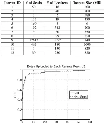
We ran between 1 and 3 experiments on 12 different torrents. Each experiment lasted for 8 hours in order to make sure that each client became a seed and to have a representative trace in seed state.
We give the characteristic of each torrent in Table I. The number of seeds and leechers is given at the beginning of the experiment. Therefore, these numbers can be much different at the end of the experiment. Whereas these torrents have very different characteristics, we found surprisingly a very stable behavior of the protocol. Due to space limitations we cannot
3Between 0% to 16% of the IP addresses, depending on the experiments,
are associated in our traces to more than one peer ID, the mean is around 7%.
TABLE I
TORRENTS CHARACTERISTICS.
Torrent ID # of Seeds # of Leechers Torrent Size (MB)
1 50 18 600 2 1 40 800 3 1 2 580 4 115 19 430 5 160 5 6 6 102 342 200 7 9 30 350 8 1 29 350 9 12612 7052 140 10 462 180 2600 11 1 130 820 12 30 230 820 0 10 20 30 40 50 60 0 0.2 0.4 0.6 0.8 1 MBytes CDF
Bytes Uploaded to Each Remote Peer, LS
All No Seed
Fig. 1. CDF of the number of bytes uploaded to each remote peer when the local peer is in leecher state.
present the results for each experiment. Instead, we illustrate each important result with a figure representing the behavior of a representative torrent, and we discuss the differences of behavior for the other torrents.
IV. EXPERIMENTATIONRESULTS
A. Choke Algorithm
In the following figures, the legend all represents the population of all peers that were in the peer set during the experiment, i.e., all the leechers and all the seeds. The legend
no seed represents the population of all peers that were in the
peer set in the experiment, but that were not initial seed, i.e., seed the first time they joined the peer set. In particular, the
no seed peers can become seed during the experiment after
they first join the peer set of the local peer.
The all population gives a global view over all peers, but does not allow to make a distinction between seeds and leechers. However, it is important to identify the seeds among the set of peers that do not receive anything from the local peer, because by definition seeds cannot receive any piece. To make this distinction, the no seed population that does not contain the initial seeds is presented along with the all population in figures.
All the figures in this section are given for torrent 7. The local peer spent 562 minutes in the torrent. It stayed 228 minutes in leecher state and 334 minutes in seed state.
0 20 40 60 80 0 10 20 30 40 50 60 Peer ID MBytes
Bytes Uploaded to Each Remote Peer, LS All No Seed
Fig. 2. Aggregate amount of bytes uploaded to each remote peer when the local peer is in leecher state.
0 20 40 60 80 0 200 400 600 800 1000 1200 Peer ID Number of Unchokes
Unchokes in Leecher State RU OU
Fig. 3. Number of times each peer is unchoked when the local peer is in the leecher state.
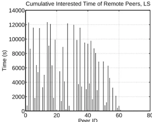
1) Leecher State: Fig. 1 represents the CDF of the number
of bytes uploaded to each remote peer, when the local peer is in leecher state. The solid line represents the CDF for all peers and the dashed line represents the CDF for all the no
seed peers. Fig. 2 represents the aggregate amount of bytes
uploaded to each remote peer, when the local peer is in leecher state. Fig. 3 shows the number of times each peer is unchoked either as regular unchoke (RU) or as optimistic unchoke (OU). Peer IDs for Fig. 2 and Fig. 3 are ordered according to the time the peer is discovered by the local peer, first discovered peer with the lowest ID. All peers IDs for the entire experiment are given.
We see in Fig. 1 that most of the peers receive few bytes, and few peers receive most of the bytes. There are 42% of all peers and 31% of the no seed peers that do not receive any byte from the local peer. We see in Fig. 2 that the population size of all peers is 79, i.e., there are 79 peers seen by the local peer during the entire experiment. The population size of the
no seed peers is 67, i.e., there are 12 initial seeds in the all
peers population. These initial seeds are identified as a cross without a circle around in Fig. 2.
We say that the local peer discovers a remote peer when this remote peer enters for the first time the peer set. All the initial seeds were discovered by the local peer before the seed state, but 18 other peers were discovered after the seed state for both the all and no seed populations. Thus, these 18 peers
0 20 40 60 80 0 2000 4000 6000 8000 10000 12000 14000
Cumulative Interested Time of Remote Peers, LS
Peer ID
Time (s)
Fig. 4. Cumulative interested time of the remote peers in the pieces of the local peer, when the local peer is in leecher state.
cannot receive any bytes from the local peer in leecher state. These peers are the peers with ID 62 to 79 in Fig. 2 and Fig. 3. Finally, only three peers (peers with ID 29, 59, and 61) were discovered before the seed state and were not seed, but did not receive any byte from the local peer. Fig. 4 shows the cumulative interested time of the remote peers in the pieces of the local peer, when the local peer is in leecher state. Peers with ID 29 and 61 were interested in the local peer, i.e., had a chance to be unchoked by the local peer, respectively 9 seconds and 120 seconds. They were never unchoked due to a too short interested time. The peer with ID 59 was interested 408 seconds in the local peer and were optimistically unchoked 3 times. However, this peer never sent a request for a block to the local peer. This is probably due to an overloaded or misbehaving peer. For all peers 18+12+379 ≈ 42% of the peers
and for the no seed peers 18+367 ≈ 31% of the peers did not
receive anything, which matches what we see in Fig. 1. In summary, few peers receive most of the bytes, most of the peers receive few bytes. The peers that do not receive anything are either initial seeds, or not interested enough in the pieces of the local peer. This result is a direct consequence of the choke algorithm in leecher state. We see in Fig. 3 that most of the peers are optimistically unchoked, and few peers are regularly unchoked a lot of time. The peers that are not unchoked at all are either initial seeds, or peers that do not stay in the peer set long enough to be optimistically unchoked, or peers that are no interested in the pieces of the local peer. After 600 seconds of experiment and up to the end of the leecher state, a minimum of 18 and a maximum of 28 peers are interested in the local peer. In leecher state, the local peer is interested to a minimum of 19 and a maximum of 37 remote peers. Therefore, the result is not biased due to a lack of peers, or to a lack of interest.
The observed behavior of the choke algorithm in leecher state is the exact expected behavior. The optimistic unchoke gives a chance to all peers, and the regular unchoke keeps unchoked the remote peers from which the local peer gets the highest download rate.
Because the choke algorithm takes its decisions based on the current download rate of the remote peers, it does not achieve a perfect reciprocation of the amount of bytes downloaded
0 10 20 30 40 0
50 100
Down (MB)
Correlation Download, Upload, and Unchoke
0 10 20 30 40 0 50 100 Up (MB) 0 10 20 30 40 0 1 2x 10 4 Ordered Peer ID Time (s)
Fig. 5. Correlation between the downloaded bytes, uploaded bytes, and unchoked time in leecher state.
0 5 10 15 20 25 0 0.2 0.4 0.6 0.8 1 MBytes CDF
Bytes Uploaded to Each Remote Peer, SS
All No Seed
Fig. 6. CDF of the number of bytes uploaded to each remote peer when the local peer is in seed state.
and uploaded. Fig. 5 shows the relation between the amount of bytes downloaded from leechers (top subplot), the amount of bytes uploaded (middle subplot), and the time each peer is unchoked (bottom subplot). Peers are ordered according to the amount of bytes downloaded, the same order is kept for the two other subplots. We see that the peers from which the local peer downloads the most are also the peers the most frequently unchoked and the peers that receive the most uploaded bytes. Even if the reciprocation is not strict, the correlation is quite remarkable.
We observed a similar behavior of the choke algorithm in leecher state for all the experiments we performed.
2) Seed State: Fig. 6 represents the CDF of the number
of bytes uploaded to each remote peer, when the local peer is in seed state. The solid line represents the CDF for all peers and the dashed line represents the CDF for all the no
seed peers. We see that the shape of the curve significantly
differs from the shape of the curve in Fig. 1. The amount of bytes uploaded to each peer is uniformly distributed among the peers. This uniform distribution is a direct consequence of time spent by each peer in the peer set. The choke algorithm gives roughly to each peer the same service time. However, when a peer leaves the peer set, it receives a shorter service time than a peer that stays longer. Fig. 7 shows the CDF of the time spent in the peer set. We observe that the curve can be linearly approximated with a given slope between 0 and 13,680
0 1 2 3 4 x 10⁴ 0 0.2 0.4 0.6 0.8 1 Time (s) CDF
Time Spent in the Peer Set
Fig. 7. CDF of the time spent in the peer set.
0 20 40 60 80 0 100 200 300 400 500 Peer ID Number of Unchokes
Unchokes in Seed State SRU SKU
Fig. 8. Number of time each peer is unchoked when the local peer is in the seed state.
seconds (228 minutes), i.e., when the peer is in leecher state, and with another slope from 13,680 seconds up to the end of the experiment, i.e., when the local peer is in seed state. The change in the slope is due to seeds leaving the peer set when the local peer becomes a seed. Indeed, when a leecher becomes a seed, it removes from its peer set all the seeds. The time spent in the peer set in seed state follows a uniform distribution as the shape of the CDF is linear. Therefore, the number of bytes uploaded to each remote peer shall follow the same distribution, which is confirmed by Fig. 6.
The uniform distribution of the time spent in the peer set is not a constant in our experiments. For some experiments, the CDF of the time spent in the peer set is more concave, indicating that some peers spend a longer time in the peer set, whereas most of the peers spend a shorter time compared to a uniform distribution. However, we observe the same behavior of the choke algorithm in seed state for all experiments. In particular, the shape of the CDF of the number of bytes uploaded to each remote peer closely match the shape of the CDF of the time spent in the peer set when the local peer is in seed state. Therefore, the service time given by the choke algorithm in seed state depends linearly on the time spent in the peer set.
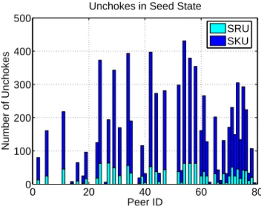
Fig. 8 shows the number of time each peer is unchoked either as seed random unchoke (SRU) or as seed keep unchoke (SKU). We see that the number of unchokes is well balanced
among the peers in the peer set. SRUs account for a small part of the total number of unchokes. Indeed, this type of unchoke is only intended to give a chance to a new peer to enter the active peer set. Then this peer remains a few rounds in the active peer set as SKU. The peer leaves the active peer set when four new peers are unchoked as SRU more recently than itself. It can also prematurely leave the active peer set in case it does not download anything during a round.
We see that with the new choke algorithm in seed state, a peer with a high download capacity can no more lock a seed. This is a significant improvement of the algorithm. However, as only the mainline client implements this new algorithm, it is not yet possible to evaluate its impact on the overall efficiency of the protocol on real torrents.
We will now discuss the impact of the choke algorithm in seed state on a torrent. A peer can download from leechers and from seeds, but the choke algorithm cannot reciprocate to seeds, as seeds are never interested. As a consequence, a peer downloading most of its data from seeds will correctly reciprocate to the leechers it downloads from, but its contri-bution to the torrent in leecher state will be lower than in the case it is served by leechers only. Indeed, when the local peer has a high download capacity and it downloads most of its data from seeds, this capacity is only used to favor itself (high download rate) and not to contribute to the torrent (low upload time) in leecher state. Without such seeds, the download time would have been longer, thus a longer upload time, which means a higher contribution to the torrent in leecher state. Moreover, as explained in section II-C.1, when the local peer has a high download capacity, it can attract and monopolize a seed implementing the old choke algorithm in seed state.
In our experiments we found several times a large amount of data downloaded from seeds for torrents with a lot of leechers and few seeds. For instance, for an experiment on torrent 12, the local peer downloaded more than 400 MB from a single seed for a total content size of 820 MB. The seed was using a client with the old choke algorithm in seed state. For few experiments, we found a large amount of bytes downloaded from seeds with a version of the BitTorrent client with the new choke algorithm (mainline client 4.0.0 and higher). These experiments were launched on torrents with a higher number of seeds than leechers, e.g., torrent 1 or torrent 10. In such cases, the seeds have few leechers to serve, thus the new choke algorithm does not have enough leechers in the peer set to perform a noticeable load balancing. That explains the large amount of bytes downloaded from seeds even with the new choke algorithm.
For one experiment on torrent 5, the local peer downloaded exclusively from seeds. This torrent has a lot of seeds and few leechers. The peer set of the local peer did not contain any leecher. Even if in such a case, the local peer cannot contribute, as there is no leecher in its peer set, it can adversely monopolize the seeds implementing the old choke algorithm in seed state.
In summary, the choke algorithm in seed state is as im-portant as in leecher state to guarantee a good reciprocation. The new choke algorithm is more robust to free riders and to misbehaviors than the old one.
3) Summary of the Results on the Choke Algorithm: The
choke algorithm is at the core of the BitTorrent protocol. Its impact on the efficiency of the protocol is hard to understand, as it depends on many dynamic factors that are unknown: remote peers download capacity, dynamics of the peers in the peer set, interested and interesting state of the peers, bottlenecks in the network, etc. For this reason, it hard to state, without doing a real experiment, that the short time scale reciprocation of the choke algorithm can lead to a reasonable reciprocation in a time scale spanning the whole torrent experiment.
We found that in leecher state: i)All leechers get a chance to join the active peer set; ii)Only a few leechers remain a significant amount of time in the active peer set; iii)For those leechers, there is a good reciprocation between the amount of bytes uploaded and downloaded.
We found that in seed state: i)All leechers get an equal chance to stay in the active peer set; ii) The amount of data uploaded to a leecher is proportional to the time the leecher spent in the peer set; iii) The new choke algorithm performs better than the old one. In particular it is robust to free riders, and favors a better reciprocation.
One fundamental requirement of the choke algorithm is that it can always find interesting peers and peers that are inter-ested. A second requirement is that the set of peers interesting and the set of peers interested is quite stable, at a time scale larger than a choke algorithm round. If these requirements are not fulfilled, we cannot make any assumption on the outcome of the choke algorithm. For this reason, a second algorithm is in charge to guarantee that both requirements are fulfilled: the rarest first algorithm.
B. Rarest First Algorithm
The rarest first algorithm target is to maximize the entropy of the pieces in the torrent, i.e., the diversity of the pieces among peers. In particular, it should prevent pieces to become rare pieces, i.e., pieces with only one copy, or significantly less copies than the mean number of copies. A high entropy is fundamental to the correct behavior of the choke algorithm [9].
The rarest first algorithm should also prevent the last pieces problem, in conjunction with the end game mode. We say that there is a last pieces problem when the download speed suffers a significant slow down for the last pieces.
1) Rarest Piece Avoidance: The following figures are the
results of an experiment on torrent 7. The content distributed in this torrent is split in 1395 pieces.
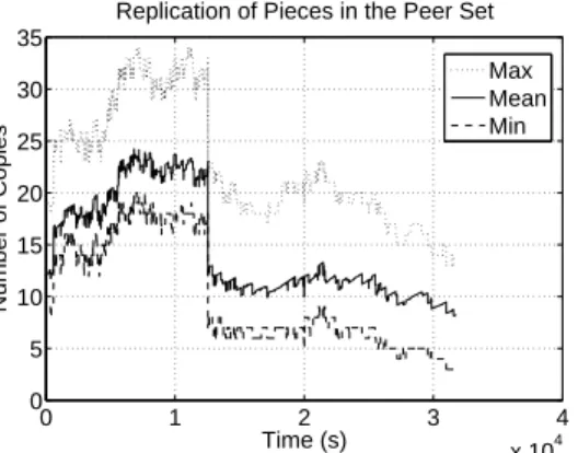
Fig. 9 represents the evolution of the number of copies of pieces in the peer set with time. The dotted line represents the number of copies of the most replicated piece in the peer set at each instant. The solid line represents the average number of copies over all the pieces in the peer set at each instant. The dashed line represents the number of copies of the least replicated piece in the peer set at each instant. The most and least replicated pieces change over time. Despite a very dynamic environment, the mean number of copies is well bounded by the number of copies of the most and
0 1 2 3 4 x 10⁴ 0 5 10 15 20 25 30 35
Replication of Pieces in the Peer Set
Time (s)
Number of Copies
Max Mean Min
Fig. 9. Evolution of the number of copies of pieces in the peer set.
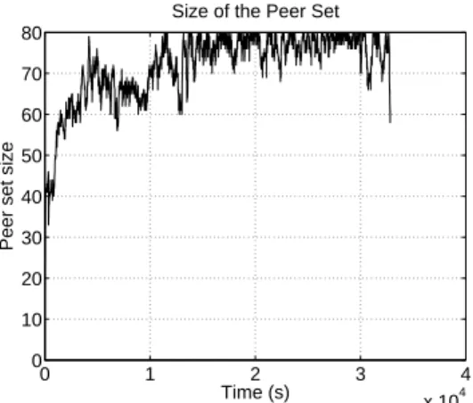
0 1 2 3 4 x 10⁴ 0 5 10 15 20 25 30 35 40 Time (s)
Peer set size
Size of the Peer Set
Fig. 10. Evolution of the peer set size.
least replicated pieces. In particular, the number of copies of the least replicated piece remains close to the average. The decrease in the number of copies 13680 seconds (228 minutes) after the beginning of the experiment corresponds to the local peer switching to seed state. Indeed, when a peer becomes seed, it closes its connections to all the seeds, following the BitTorrent protocol.
The evolution of the number of copies closely follows the evolution of the peer set size as shown in Fig. 10. This is a hint toward the independence between the number of copies in the peer set and the identity of the peers in the set. Indeed, with a high entropy, any subset of peers shall have the same statistical properties, e.g., the same mean number of copies.
We see in Fig. 9 that even if the min curve closely follows the mean, it does not significantly get closer. However, the rarest first algorithm does a very good job at increasing the number of copies of the rarest pieces. To support this claim we have plotted over time the number of rarest pieces, i.e., the set size of the pieces that are equally rarest. Fig. 11 shows this curve. We have removed from the data the first second, as when the first peer joins the peer set and it is not a seed, the number of rarest pieces can reach high values.
We see in this figure a sawtooth behavior that is represen-tative of the behavior of the rarest first algorithm. Each peer joining or leaving the peer set can alter the set of rarest pieces. However, as soon as a new set of pieces becomes rarest, the rarest first algorithm quickly duplicates them as shown by a
0 0.5 1 1.5 2 2.5 3 x 10⁴ 0 20 40 60 80 100
Number of Rarest Pieces
Time (s)
Num. rarest
Fig. 11. Evolution of the number of rarest pieces in the peer set.
0 1 2 3 4 x 10⁴ 0 10 20 30 40 50 60
Replication of Pieces in the Peer Set
Time (s)
Number of Copies
Max Mean Min
Fig. 12. Evolution of the number of copies of pieces in the peer set for torrent 11.
consistent drop of the number of rarest pieces in Fig.11. We observed the same behavior for almost all our ex-periments. However, for a few experiments, we encountered periods with some pieces missing in the peer set. To illustrate this case, we now focus on results of an experiment performed on torrent 11. The file distributed in this torrent is split in 1657 pieces. We run this experiment during 32828 seconds. At the beginning of the experiment there were 1 seed and 130 leechers in the torrent. After 28081 seconds, we probed the tracker for statistics and found 1 seed and 243 leechers. After 32749 seconds we found 16 seeds and 222 leechers in the torrent. As a consequence, this torrent had only one seed for the duration of most of our experiment. Moreover, in the peer set of the local peer, there was no seed in the intervals [0,2594] seconds and [13783,32448] seconds.
Fig. 12 represents the evolution of the number of copies of pieces in the peer set with time. We see some major differences compared to Fig. 9. First, the number of copies of the least replicated piece is often equal to zero. This means that some pieces are missing in the peer set. Second, the mean number of copies is significantly lower than the number of copies of the most replicated piece. Unlike what we observed in Fig. 9, the mean curve does not follow a parallel trajectory to the max curve. Instead, it is continuously increasing toward the max curve, and does not follow the same trend as the peer set size shown in Fig. 13. As the mean curve increase is not
0 1 2 3 4 x 10⁴ 0 10 20 30 40 50 60 70 80 Time (s)
Peer set size
Size of the Peer Set
Fig. 13. Evolution of the peer set size for torrent 11.
0 1 2 3 4 x 10⁴ 0 200 400 600 800 1000 1200 1400
Number of Rarest Pieces
Time (s)
Num. rarest
Fig. 14. Evolution of the number of rarest pieces in the peer set for torrent 11.
due to an increase in the number of peers in the peer set, this means that the rarest first algorithm increases the entropy of the pieces in the peer set over time.
In order to gain a better understanding of the replication process of the pieces for torrent 11, we plotted the evolution in the peer set of the local peer of the number of rarest pieces over time in Fig. 14 and of the number of missing pieces over time in Fig. 15. Whereas the former simply shows the replication of the pieces within the peer set of the local peer, the later shows the impact of the peers outside the peer set on the replication of the missing pieces within the peer set.
We see in Fig. 14 that the number of rarest pieces decreases linearly with time. As the size of each piece in this torrent is 512 kB, a rapid calculation shows that the rarest pieces are duplicated in the peer set at a rate close to 20 kB/s. The exact rate is not the same from experiment to experiment, but the linear trend is a constant in all our experiments. As we only have traces of the local peer, but not of all the peers in the torrent, we cannot identify the peers outside the peer set contributing pieces to the peers in the peer set. For this reason it is not possible to give the exact reason of this linear trend. Our guess is that, as the entropy is high, the number of peers that can serve the rarest pieces is stable. For this reason, the capacity of the torrent to serve the rarest pieces is constant, whatever the peer set is.
Fig. 12 shows that the least replicated piece (min curve) has
0 1 2 3 4 x 10⁴ 0 200 400 600 800 1000 1200 1400
Number of Missing Pieces in the Peer Set
Time (s)
Num. missing
Fig. 15. Evolution of the number of missing pieces in the peer set for torrent 11. 10−2 10−1 100 101 102 0 0.2 0.4 0.6 0.8 1 Time (s) CDF
Block Interarrival Time
All blocks 100 first 100 last
Fig. 16. CDF of the block interarrival time.
a single copy in the peer set when the seed is in the peer set and is missing when the seed leaves the peer set. Therefore, the rarest pieces set for this experiment contains pieces that are at most present on a single peer in the peer set of the local peer. Fig. 15 complements this result. We see that each time the seed leaves the peer set, a high number of pieces is missing. When the seed is not in the peer set, the source of the rarest pieces is outside the peer set, as the rarest pieces are the missing pieces. However, the local peer perceived decrease rate of the rarest pieces does not change from the beginning up to 30000 seconds. That confirms that the capacity of the torrent to serve the rarest pieces is stable, whatever the peer set for each peer is.
In conclusion, our guess is that with the rarest first policy, the pieces availability in the peer set is independent of the peers in this set. All our experimental results tend to confirm this guess. However, a global view of the torrent is needed to confirm this guess. Whereas it is beyond the scope of this paper to evaluate globally a torrent, this is an interesting area for future research.
2) Last Piece Problem: The rarest first algorithm is
some-times presented as a solution to the last piece problem [13]. We evaluate in this section whether the rarest first algorithm solves the last piece problem. We give results for an experi-ment on torrent 7 and discuss the differences with the other experiments.
10−2 10−1 100 101 102 103 104 0 0.2 0.4 0.6 0.8 1 Time (s) CDF
Piece Interarrival Time
All pieces 100 first 100 last
Fig. 17. CDF of the piece interarrival time.
solid line represents the CDF for all blocks, the dashed line represents the CDF for the 100 first downloaded blocks, and the dotted line represents the CDF for the 100 last downloaded blocks. We first see that the curve for the last 100 blocks is very close to the one for all blocks. The interarrival time for the 100 first blocks is larger than for the 100 last blocks. For a total of 22308 blocks4 around 83% of the blocks have a interarrival time lower than 1 second, 98% of the blocks have an interarrival time lower than 2 seconds, and only three blocks have an interarrival time higher than 5 seconds. The highest interarrival time among the last 100 blocks is 3.47 seconds. Among the 100 first blocks we find the two worst interarrival time.
We have never observed a last blocks problem in all our experiments. As the last 100 blocks do not suffer from a significant interarrival time increase, the local peer did not suffer from a slow down at the end of the download. However, we found several times a first blocks problem. This is due to the startup phase of the local peer, which depends on the set of peers returned by the tracker and the moment at which the remote peers decide to optimistically unchoke or seed random
unchoke the local peer. We discuss in section IV-B.3 how
experimental clients improve the startup phase.
A block is the unit of data transfer. However, partially received pieces cannot be retransmitted by a BitTorrent client, only complete pieces can. For this reason it is important to study the piece interarrival time, which is representative of the ability of the local peer to upload pieces. Fig. 17 shows the CDF of piece interarrival time. The solid line represents the CDF for all pieces, the dashed line represents the CDF for the 100 first downloaded pieces, and the dotted line represents the CDF for the 100 last downloaded pieces. We see that there is no last pieces problem. We observed the same trend in all our experiments. The interarrival time is lower than 10 seconds for 68% of the pieces, it is lower than 30 seconds for 97% of the pieces, and only three pieces have an interarrival time larger than 50 seconds.
Fig. 18 shows the CDF of the interarrival time between the first and last received blocks of a piece for each piece. The
4Each piece is split into a fixed number of blocks, except the last piece that
can be smaller depending on the file size. In this case, there are 1394 pieces split into 16 blocks and the last piece is split into 4 blocks.
100 101 102 103 104 0 0.2 0.4 0.6 0.8 1 Time (s) CDF
Interarrival Time: First/Last Block for each Piece
Single peer Multi peers All
Fig. 18. CDF of the interarrival time of the first and last received blocks for each piece. 10−1 100 101 102 103 104 105 0 0.2 0.4 0.6 0.8 1 Throughput (KBytes/s) CDF
Pieces and Blocks Download Throughput
Block Piece
Fig. 19. CDF of the pieces and blocks download throughput.
solid line shows the CDF for all the pieces, the dashed line represents the CDF for the pieces served by a single peer, the dotted line represents the CDF for the pieces served by at least two different peers. We see that pieces served by more than one peer have a higher first to last block piece interarrival time than pieces served by a single peer. The maximum interarrival time in the case of the single peer download is 556 seconds. In case of a multi peers download, 7.6% of the pieces have a first to last received block interarrival time larger than 556 seconds, and the maximum interarrival time is 3343 seconds. As the local peer cannot upload pieces partially received, a large interarrival time between the first and last received blocks is suboptimal.
It is important to evaluate the impact of a large interarrival time between the first and last received blocks on the piece interarrival rate. Fig. 19 shows the CDF of the pieces down-load throughput and of the blocks downdown-load throughput. We compute the blocks (resp. pieces) download throughput CDF by dividing the block (resp. piece) size by the block (resp. piece) interarrival time for each interarrival time. We see that both CDF closely overlap, meaning that the blocks and pieces download throughput is roughly equivalent. Consequently, the constraint to send pieces only, but not blocks, does not lead to a significant loss of efficiency.
Fig. 20 represents the CDF of the pieces served by n different peers. The solid line represents the CDF for all pieces, the dashed line represents the CDF for all pieces
1 2 3 4 5 6 7 0 0.2 0.4 0.6 0.8 1 Number of Peers CDF
Number Pieces Served by N Different Peers, NZ
All Before EG After EG
Fig. 20. CDF of the number of pieces served by a different number of peers.
downloaded before the end game mode, and the dotted line represents the CDF of the pieces downloaded once in end game mode. We see that a significant portion of the pieces are downloaded by more than a single peer. Some pieces are downloaded from 7 different peers. We note that the end game mode does not lead to an increase in the number of peers that serve a single piece. As the end game mode is activated for the last few blocks to download, the respective percentage of pieces served by a single peer or several peers in end game mode is not significant. Whereas the end game mode triggers a request for the last blocks to all peers in the peer set, we see in all our experiments that the end game mode does not lead to a piece downloaded by more peers than before the end game mode.
All the results in this section are given for an experiment on torrent 7. However, we did not observe any fundamental differences in the other experiments. The major difference is the absolute interarrival time that decreases for all the plots when the download speed of the local peer increases.
We have not evaluated the respective merits of the rarest first algorithm and of the end game mode. We do not expect to see a major impact of the end game mode. First, the end game mode is only activated for the last few blocks, thus a very low impact on the overall efficiency. Second, this mode is useful in case of pathological cases, when the last pieces are downloaded from a slow peer. Whereas a user can tolerate a slowdown during a download, it can be frustrating to see it at the end of the download. The end game mode acts more as a psychological factor than as a significant improvement of the overall BitTorrent download speed.
3) Summary of the Results on the Rarest First Algorithm:
The rarest first algorithm is at the core of the BitTorrent protocol, as important as the choke algorithm. The rarest first algorithm is simple and based on local decisions.
We found that: i)The rarest first algorithm increases the entropy of pieces in the peer set; ii)The rarest first algorithm does a good job at attracting missing pieces in a peer set; iii)The last pieces problem is overstated, but the first pieces problem is underestimated.
We saw that multi peer download of a single piece does not impact significantly the pieces download speed of the local peer. With the rarest first algorithm, rarest pieces are
down-0 2000 4000 6000 8000 10000 12000 0 0.2 0.4 0.6 0.8 1 Time (s) CDF
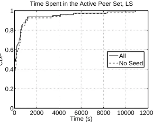
Time Spent in the Active Peer Set, LS
All No Seed
Fig. 21. CDF of the time spent by remote peers in the active peer set in leecher state.
loaded first. Thus, in case the remote peer stops uploading data to the local peer, it is possible that the few peers that have a copy of the piece do not want to upload it to the local peer. However, the strict priority policy mitigates successfully this drawback of the rarest first algorithm.
Finally, we have seen that whereas we did not observe a last pieces problem, we observed a first pieces problem. The first pieces take time to download, when the initial peer set returned by the tracker is too small. In such a case, the Azureus client offers a significant improvement. Indeed, with Azureus, peers can exchange their peer set during the initial peer handshake performed to join the peer set of the local peer. This results in a very fast growth of the peer set as compared to the mainline client. We have not evaluated in detail this improvement, but it is an interesting problem for future research.
C. Peer Set and Active Peer Set Evolution
In this section, we evaluate the dynamics of the peer set and of the active peer set. This dynamics is important as it captures most of the variability of the torrent. These results provide also important insights for the design of realistic models of BitTorrent. All the figures in this section are given for torrent 7.
1) Active Peer Set: The dynamics of the active peer set
depends on the choke algorithm, but also on the dynamics of the peers, and on the pieces availability. In this section, we study the dynamics of the active peer set on real torrents.
In the following figures, all represents all peers that were in the peer set during the experiments, and no seed represents all the peers that were in the peer set in the experiment, but that were not seed the first time they joined the peer set.
Fig. 21 represents the CDF of the time spent by the remote peers in the active peer set of the local peer when it is in leecher state. We observe a CDF very close to the one of Fig. 1. It was indeed observed in section IV-A.1 that there is a strong correlation between the time spent in the active peer set and the amount of bytes uploaded to remote peers. The main difference between Fig. 1 and Fig. 21 is that the peer with ID 59 was unchoked, but did not receive any block. As a consequence, for all peers 18+12+279 ≈ 40% of the peers and for the no seed peers 18+267 ≈ 30% of the peers are never in the active peer set (see section IV-A.1 for a detailed discussion on the all and no seed populations).
0 1000 2000 3000 4000 5000 0 0.2 0.4 0.6 0.8 1 Time (s) CDF
Time Spent in the Active Peer Set, SS
All No Seed
Fig. 22. CDF of the time spent in the active peer set in seed state.
In Fig. 3, we see that few peers stay a long time in the active peer set as regular unchoke, and the optimistic unchoke gives most of the peers a chance to join the active peer set. In summary, the active peer set is stable for the three peers that are unchoked as regular unchoke, the additional peer unchoked as optimistic unchoke changes frequently and can be approximated as a random choice in the peer set. This conclusion is consistent with all our experiments.
Fig. 22 represents the CDF of the time spent by remote peers in the active peer set of the local peer when it is in seed state. We see a CDF very close to the one of Fig. 6. There is indeed a strong correlation between the time spent in the active peer set and the amount of bytes uploaded to remote peers.
As explained in section IV-A.2, the distribution of the time spent in the active peer set in seed state is similar to the distribution of the time spent in the peer set in seed state. An analogous behavior has been observed in all our experiments. In particular, the CDF of the time spent by remote peers in the active peer set of the local peer when it is in seed state (Fig. 22), the CDF of the number of bytes uploaded to each remote peer when the local peer is in the seed state (Fig. 6), and the CDF of the time spent in the peer set (Fig. 7) have the same shape. In the next section we evaluate the dynamics of the peer set in our experiments.
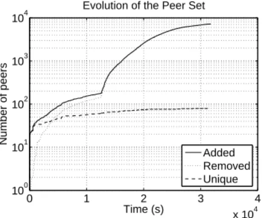
2) Peer Set: Fig. 10 represents the evolution of the peer set
size with time. The peer set size decreases 13680 seconds after the start of the experiment, which corresponds to the local peer switching to seed state. We see that the peer set size has a lot of small variations, in particular when the local peer is in seed state. To explain this behavior, we have plotted the cumulative number of peers joining and leaving the peer set with time in Fig. 23. The solid line is the cumulative number of times a peer joins the peer set, the dotted line is the cumulative number of times a peer leaves the peer set, and the dashed line is the cumulative number of times a unique peer (identified by its IP address and client ID) joins the peer set.
We first note the huge difference between the cumulative number of joins and the cumulative number of unique peer joining the peer set. The difference grows when the local peer switches to seed state. This difference is due to a misbehavior
0 1 2 3 4 x 10⁴ 100 101 102 103 104 Time (s) Number of peers
Evolution of the Peer Set
Added Removed Unique
Fig. 23. Evolution of the peer set population.
of popular BitTorrent clients5. When a local peer becomes a seed, it disconnects from all the seeds in its peer set. The
mainline client reacts to such a disconnect by dropping the
connection. Instead, the misbehaving clients try to reconnect. Whereas this behavior could make sense when the local peer is in leecher state, it is meaningless when the remote peer becomes a seed. As the frequency of the reconnect is small, this behavior generates a large amount of useless messages. However, compared to the amount of regular messages, these useless messages are negligible.
Fig. 23 shows a slow increase of the unique peers joining the peer set. At the end of the experiment, 79 different peers have joined the peer set. This result is consistent with all the other experiments. Moreover, the increase of the unique peers joining the peer set follows a linear trend with time. The only exceptions are when the number of different peers reaches the size of the torrent. In this case, the curve flattens. This result is important as it means that the amount of new peers injected in the peer set is roughly constant with time. We do not have any convincing explanation for this trend, and we intend to further investigate this result in the future.
D. Protocol Overhead
There are 11 messages in BitTorrent6 as specified by the
mainline client in version 4.0.x. All the messages are sent
using TCP. In the following, we give a brief description of the BitTorrent messages, the size of each message is given without the TCP/IP header overhead of 40 bytes.
• The HANDSHAKE (HS) message is the first message exchanged when a peer initiates a connection with a remote one. The initiator of the connection sends a
HANDSHAKE message to a remote peer. The remote peer
answers with another HANDSHAKE message. Then the connection is deemed to be setup and no more
HAND-SHAKE message is exchanged. A connection between
two peers is symmetric. If the connection is closed, a new
5We have observed this misbehavior for BitComet, Azureus, and variations
of them.
6Due to space limitations, we do not give all the details, but a rapid
survey of the different messages. The interested reader is referred to the documentation available on the BitTorrent Web site [10].
handshake is required to setup again this connection. The
HANDSHAKE message size is 68 bytes.
• The KEEP ALIVE (KA) message is periodically sent to each remote peer to avoid a connection timeout on the connection to this remote peer. The KEEP ALIVE message size is 4 bytes.
• The CHOKE (C) message is sent to a remote peer the local peer wants to choke. The CHOKE message size is 5 bytes.
• The UNCHOKE (UC) message is sent to a remote peer the local peer wants to unchoke. The UNCHOKE message size is 5 bytes.
• The INTERESTED (I) message is sent to a remote peer when the local peer is interested in the content of this remote peer. The INTERESTED message size is 5 bytes.
• The NOT INTERESTED (NI) message is sent to a remote peer when the local peer is not interested in the content of this remote peer. The NOT INTERESTED message size is 5 bytes.
• The HAVE (H) is sent to each remote peer when the local peer has received a new piece. It contains the new piece ID. The HAVE message size is 9 bytes.
• The BITFIELD (BF) message is sent only once after each handshake to notify the remote peer of the pieces the local peer already has. Both the initiator of the connec-tion and the remote peer send a BITFIELD message. The BITFIELD message size is variable. Its size is a function of the number of pieces in the content and is
d# of pieces8 e + 5 bytes.
• The REQUEST (R) message is sent to a remote peer to request a block to this remote peer. The REQUEST message size is 17 bytes.
• The PIECE (P) message is the only one that is used to send blocks. Each PIECE message contains only one block. Its size is a function of the block size. For a default block size of 214 bytes, the size of the PIECE message will be 214+ 13 bytes.
• The CANCEL (CA) message is used during the end game mode to cancel a REQUEST message. The CANCEL message size is 17 bytes.
We have described the way local peer, remote peer. As the connections between the local peer and the remote peers are symmetric, each remote peer can be considered as a local peer from its point of view. Therefore, each remote peer will also send messages to the local peer.
We have evaluated for each experiment the protocol over-head. We count as overhead the 40 bytes of the TCP/IP header for each message exchanged plus the BitTorrent message overhead. We count as payload the bytes received or sent in a PIECE message without the PIECE message overhead. The upload overhead is the ratio of all the sent messages overhead over the total amount of bytes sent (overhead + payload). The download overhead is the ratio of all the received messages overhead over the total amount of bytes received (overhead + payload).
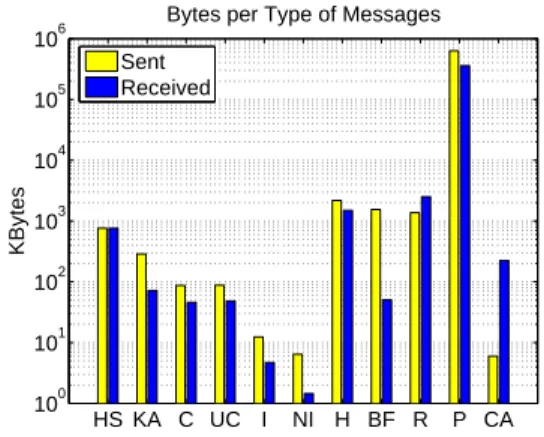
Fig. 24 shows the number of messages and Fig. 25 the number of bytes sent and received by the local peer for each type of messages for torrent 7. According to Fig. 24 the HAVE,
HS KA C UC I NI H BF R P CA 100 101 102 103 104 105
Number of Messages per Type
Num. of messages
Sent Received
Fig. 24. Messages sent from and received by the local peer per message type. HS KA C UC I NI H BF R P CA 100 101 102 103 104 105 106 KBytes
Bytes per Type of Messages Sent
Received
Fig. 25. Bytes sent from and received by the local peer per message type.
REQUEST, and PIECE messages account for most of the
messages sent and received. Fig. 25 shows that the PIECE messages account for most of the bytes sent and received far more than the HAVE, REQUEST, and BITFIELD messages. All the other messages have only a negligible impact on the overhead of the protocol. This result is consistent with all our experiments and explain the low overhead of the protocol.
Overall, the protocol download and upload overhead is lower than 2% in most of our experiments. The messages that account for most of the overhead are the HAVE, REQUEST, and BITFIELD messages. The contribution to the overhead of all other messages can be neglected in our experiments. For three experiments on torrent 5, 9, and 6, we got a download overhead of respectively 23%, 7%, and 3%, which are the highest download overhead over all our experiments. This overhead is due to the small size of the contents in these torrents (6 MB, 140 MB, 200 MB), and to a long time in seed state (8 hours). The longer the peer stays in seed state, the higher its download overhead. Indeed, in seed state a peer does not receive anymore payload data, but it continues to receive BitTorrent messages. However, even for a small content and several hours in seed state, the overhead remains reasonable.
For some experiments, we observed an upload overhead up to 15%. Several factors contribute to a large upload overhead. A small time spent in seed state reduces the amount of pieces contributed, whereas all the HAVE and REQUEST messages sent by the local peer during an experiment are sent in leecher