HAL Id: hal-01982353
https://hal.uca.fr/hal-01982353
Submitted on 31 Jan 2020
HAL is a multi-disciplinary open access
archive for the deposit and dissemination of sci-entific research documents, whether they are pub-lished or not. The documents may come from teaching and research institutions in France or
L’archive ouverte pluridisciplinaire HAL, est destinée au dépôt et à la diffusion de documents scientifiques de niveau recherche, publiés ou non, émanant des établissements d’enseignement et de recherche français ou étrangers, des laboratoires
Simultaneous measurements of electrical conductivity
and seismic wave velocity of partially molten geological
materials: effect of evolving melt texture
D. Freitas, Geeth Manthilake, J. Chantel, Mohamed Ali Bouhifd, Denis
Andrault
To cite this version:
D. Freitas, Geeth Manthilake, J. Chantel, Mohamed Ali Bouhifd, Denis Andrault. Simultaneous measurements of electrical conductivity and seismic wave velocity of partially molten geological ma-terials: effect of evolving melt texture. Physics and Chemistry of Minerals, Springer Verlag, 2019, �10.1007/s00269-019-01021-5�. �hal-01982353�
Simultaneous measurements of electrical conductivity and seismic velocity of partially 1
molten geological materials: Effect of evolving melt texture 2
D. Freitas1*, G. Manthilake1, J. Chantel2, †, M. A. Bouhifd1, D. Andrault1
3 4
1
Laboratoire Magmas et Volcans, Université Clermont Auvergne, CNRS, IRD, OPGC, F-63000
5
Clermont-Ferrand, France
6
2
UMET, Unité Matériaux Et Transformations, Bâtiment C6, University of Lille, 59655
7
Villeneuve d'Ascq, Lille, France.
8
9
*Corresponding author: (damien.freitas@uca.fr +334.73.34.67.23, ORCID:
0000-0002-1722-10 4081) 11 12 Key Points: 13
1. Electrical conductivity increases with evolving melt texture; transient melt textures can
14
underestimate the electrical conductivity.
15
2. Acoustic velocities are not strongly affected by evolving melt texture for highly wetting
16
melt
17
3. Acoustic velocities measurements are more appropriate for estimating the melt fraction.
Abstract 19
Comparison between geophysical observations and laboratory measurements yields contradicting
20
estimations of the melt fraction for the partially molten regions of the Earth, highlighting
21
potential disagreements between laboratory-based electrical conductivity and seismic wave
22
velocity measurement techniques. In this study, we performed simultaneous acoustic wave
23
velocity and electrical conductivity measurements on a simplified partial melt analogue (olivine
24
+ mid oceanic ridge basalt, MORB) at 2.5 GPa and up to 1650 K. We aim to investigate the
25
effect of ongoing textural modification of partially molten peridotite analog on both electrical
26
conductivity and sound wave velocity. Acoustic wave velocity (Vp and Vs) and EC are measured
27
on an identical sample presenting the same melt texture, temperature gradient, stress field and
28
chemical impurities. We observe a sharp decrease of acoustic wave velocities and increase of
29
electrical conductivity in response to melting of MORB component. At constant temperature of
30
1650 K, electrical conductivity gradually increases, whereas acoustic velocities remain relatively
31
constant. While the total MORB components melt instantaneously above the melting
32
temperature, the melt interconnectivity and the melt distribution should evolve with time,
33
affecting the electrical conduction. Consequently, our experimental observations suggest that
34
acoustic velocities respond spontaneously to the melt volume fraction for melt with high wetting
35
properties, whereas electrical conduction is significantly affected by subsequent melt texture
36
modifications. We find that acoustic velocity measurements are thus better suited to the
37
determination of the melt fraction of a partially molten sample at the laboratory time scale
38
(~hours). Based on our estimations, the reduced Vs velocity in the major part of the low velocity
39
zone (LVZ) away from spreading ridges can be explained by 0.3 to 0.8 vol. % volatile-bearing
melt and the high Vp/Vs ratio obtained for these melt fractions (1.82-1.87) are compatible with
41
geophysical observations.
42
Keywords: Electrical Conductivity, Acoustic Wave Velocity, Low Velocity Zone, Dihedral 43
angle, Melt fraction, MORB.
44 45
1. Introduction 46
The Earth’s asthenosphere is characterized by a region of high electrical conductivity (>
47
0.05 S/m) [Shankland and Waff, 1977], ~3-8 % reduction of acoustic wave velocity and high
48
seismic attenuation [Anderson and Sammis, 1970; Romanowicz, 1995]. A low degree of partial
49
melting has often been considered as a viable explanation (partial melting hypothesis), because
50
the magnitude of seismic and electrical anomalies cannot be explained by the temperature effect
51
alone [Fischer et al., 2010]. Alternative mechanisms based on solid state processes, such as
52
anelastic relaxation [Goetze, 1977; Stixrude and Lithgow-Bertelloni, 2005] and hydrogen
53
diffusion [Karato, 1990] in mantle minerals have also been proposed (null hypothesis). However,
54
the recent finding of young alkali basalt (< 10 Ma) on the 135 million-year-old Pacific Plate
55
[Hirano et al., 2006] provides strong physical evidence for partial melting at the top of the
56
asthenosphere.
57
The criteria for melting in the asthenosphere have been discussed in a number of recent
58
papers [Galer and O’Nions, 1986; Plank and Langmuir, 1992; Dasgupta and Hirschmann,
59
2006]. Volatile-assisted melting in the asthenosphere is favored as the mantle temperatures at the
60
relevant depths are expected to be lower than the dry peridotite solidus [Dasgupta and
61
Hirschmann, 2006]. The volatile contents of the primitive mantle samples suggest mantle
62
abundances of ~ 150 wt. ppm of H2O and ~ 100 wt. ppm of CO2 [Saal et al., 2002], while CO2
63
contents of up to 1800 wt. ppm have been reported in undegased sources [Cartigny et al., 2008].
64
The recent discovery of young alkali basalt associated with volcanism along fractures in the
65
lithosphere indicates up to 5 wt. % CO2 and 1.0 wt. % of H2O volatile contents [Okumura and
66
Hirano, 2013]. However, the measurements based on melt inclusions in minerals and quenched
67
glasses indicate a global average of about 3000 wt. ppm of H2O and 170 wt. ppm of CO2 in
natural MORB [Naumov et al., 2014]. A substantial contribution of volatiles to the melting can
69
be expected at low temperature regions in the asthenosphere [Sifré et al., 2014; Yoshino et al.,
70
2010].
71
The reduced seismic velocity and elevated electrical conductivity have been widely used
72
as evidence for the presence of melt in the Earth’s interior [Anderson and Sammis, 1970]. The
73
magnitudes of the seismic velocity and conductivity variations are directly linked to the melt
74
fraction, therefore comparison of geophysical data with laboratory models has long been
75
considered as the most plausible way to quantify the melt contents in partially molten regions of
76
the Earth [Anderson and Sammis, 1970; Shankland and Waff, 1977]. The accurate determination
77
of melt volume fraction in the asthenosphere is a key constraint for the plate tectonics and mantle
78
convection models [Schmerr, 2012]. Apart from identifying the partially molten regions and
79
quantifying the melt fractions, the seismic and electrical methods can also be used to characterize
80
their spatial distribution. For example, laboratory-based experiments [Caricchi et al., 2011;
81
Zhang et al., 2014; Pommier et al., 2015] have been able to attribute the seismic and electrical
82
anisotropies observed at spreading ridge environments to the shear localization of melt due to
83
plate motion.
84
The presence of a melt significantly modifies the viscoelastic properties of mineral
85
assemblages. The critical parameters are the volume fraction and the melt microstructures 86
[Kohlstedt, 1992]. Unfortunately, experimental determinations of seismic velocity on realistic 87
melt compositions are limited to a few studies. An early measurement of Vp and Vs in a
melt-88
bearing peridotite reported no significant effect of melt fractions below 3.0 vol. % [Sato et al.,
89
1989]. The measurements based on torsional forced oscillation of melt-bearing olivine indicate
90
reduced seismic velocities, and high attenuation can be observed for melt fractions as low as 0.01
vol.% [Faul et al., 2004], suggesting a possible melt fraction of 0.1 to 1 vol. %, for the average
92
grain size variation in the upper mantle from 1 and 10 mm, respectively. The recent experimental
93
developments allow accurate determination of seismic velocity measurements of partially molten
94
rocks at the pressure and temperature conditions expected at the Earth’s interior [Chantel et al.,
95
2016] and predicted about 0.2 vol. % melt content in the asthenosphere. On the contrary, the melt
96
fraction estimations based on the acoustic velocity of analogue systems [Takei, 2000] indicate
97
significantly higher melt fractions than those predicted using realistic upper mantle melts [Faul
98
et al., 2004; Chantel et al., 2016]. For example, the 6.6 % melt required to explain 10 % Vs
99
reduction in Borneol-diphenylamin analogue system [Takei, 2000] is considerably higher than
100
the about 1 % melt required by basaltic melt to explain a similar velocity reduction [Chantel et
101
al., 2016].
102
The dependence of acoustic wave velocities and attenuation upon melt fraction and
grain-103
scale melt distribution has also been discussed in several theoretical studies. These studies were
104
based on ideal melt geometries and explained using the oblate spheroid model [Schmeling,
105
1986], tube model [Mavko, 1980], the crack model [O’Connell and Budiansky, 1974] and models
106
based on grain boundary wetness or ‘‘contiguity’’ [Takei, 1998, 2002; Yoshino et al., 2005;
Hier-107
Majumder, 2008]. The calculations based on the finite element method on melt geometries led
108
[Hammond and Humphreys, 2000] to conclude more than 1 % melt is required to explain 3.6 %
109
and 7.9 % velocity reduction for Vp and Vs respectively, which is significantly lower than the
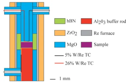
110
6.2 % and 11 % reductions observed in laboratory measurements [Chantel et al., 2016]. The
111
naturally occurring, randomly distributed melt [Faul et al., 2004; Chantel et al., 2016] is shown
112
to have a significant effect on seismic velocity compared to the simplified melt textures assumed
113
in theoretical models [Hammond and Humphreys, 2000; Takei, 2002; Yoshino et al., 2005] or
analogue systems [Takei, 2000]. The considerably higher melt volume fractions required in
115
theoretical models can be attributed to the idealized geometries, such as planar cracks, spheres,
116
ellipsoids, or simplified cuspate forms, which may not represent the true melt geometries in
117
naturally occurring melt [Kohlstedt, 1992; Faul et al., 1994; Hammond and Humphreys, 2000],
118
limiting their applications to partially molten regions in the asthenosphere.
119
An early electrical conductivity measurement on basaltic melt suggested 5-10 vol. % melt
120
needed to account for the observed electrical anomalies in the asthenosphere [Tyburczy and Waff,
121
1983]. Similar amount of basaltic melt (5%) also provided compatible values to geophysical
122
observables with values up to 0.1 S/m [Maumus et al., 2005]. However, recent studies suggest
123
the presence of much lower volume fractions; 0.3-3.0 vol. % for hydrous basaltic melt [Yoshino
124
et al., 2010; Ni et al., 2011], or less than 0.3 vol. % for carbonatitic melt [Gaillard et al., 2008;
125
Yoshino et al., 2010]. The electrical conductivity of volatile enriched basalt (15–35 wt.% CO2
126
and about 2–3 wt.% H2O) indicates about 0.1-0.15 vol.% melt could explain the observed
127
conductivity anomalies [Sifré et al., 2014]. The development of melt interconnectivity in
128
partially molten rocks is known to have a profound effect on electrical conductivity [Waff, 1974,
129
Maumus et al., 2005]. However, the number of studies investigating the influence of melt
130
microstructures on EC is extremely limited. The study by [ten Grotenhuis et al., 2005] showed
131
that a melt geometry evolving from isolated triple junction tubes at 0.01 % of melt to a network
132
of interconnected grain boundary melt layers at 0.1% of melt has a greater effect on electrical
133
conductivity.
134
Various other experimental techniques have been used to constrain the melt fraction
135
associated with the LVZ in the Earth’s asthenosphere. Geochemical constraints from trace
136
elements partitioning suggest that low degree of melting (less than 1 %) can be generated at
greater depth (below than 100 km) [Salters and Hart, 1989]. Similarly, studies based on
138
experimental petrology, such as volatile (H2O and CO2) effect on peridotite solidus, indicate the
139
melt fraction in the asthenosphere LVZ has to be 0.1 vol. % or less [Plank and Langmuir, 1992,
140
Dasgupta and Hirschmann, 2007].
141
Both experimental and theoretical models acknowledge that the volume fraction and
142
spatial distribution of melt play an integral part in modifying the seismic and electrical properties
143
of partially molten rocks. However, large discrepancies still remain in the laboratory estimations
144
(regardless of the technique) of the amount of melt volume fraction present in the asthenosphere
145
[Pommier and Garnero, 2014; Karato, 2014]. Due to the large number of studies addressing the
146
electrical properties of melt, the disagreement between laboratory-based electrical conductivity
147
measurements is highly visible [Karato, 2014]. The influence of volatile contents could be one of
148
the key parameters controlling the conductivity of the resulting melt [Yoshino et al., 2010; Ni et
149
al., 2011; Sifré et al., 2014]. A model based on chemical variation in the melt has been proposed
150
to explain the apparent disagreement on melt fraction estimations between electrical conductivity
151
measurements and seismic models [Pommier and Garnero, 2014]. The discrepancy may
152
primarily stem from the absence of systematic experimental investigation into the structural
153
factors influencing the EC in partially molten systems. The effect of melt fraction on seismic
154
velocity has been mostly limited to numerical models. Significant disagreement between these
155
theoretical models is still present due to the choice of melt geometries [Yoshino et al., 2005]. A
156
comparison with recent laboratory-based seismic velocity measurements on realistic partially
157
molten materials [Chantel et al., 2016] indicates a significant underestimation of seismic
158
response by theoretical models [Takei, 2000; Yoshino et al., 2005]. The cross-correlation of melt
fraction estimations based on theoretical seismic models and laboratory electrical conductivity is
160
at present a highly uncertain exercise.
161
The effect of melt texture and chemical compositions (volatiles) have long been assumed
162
for the observed inconsistency, but there has never been a systematic study on how the evolving
163
melt textures influence the electrical conductivity and seismic velocity (SV). Similar, melt
164
textures and melt contents during high pressure, high temperature experiments are strongly
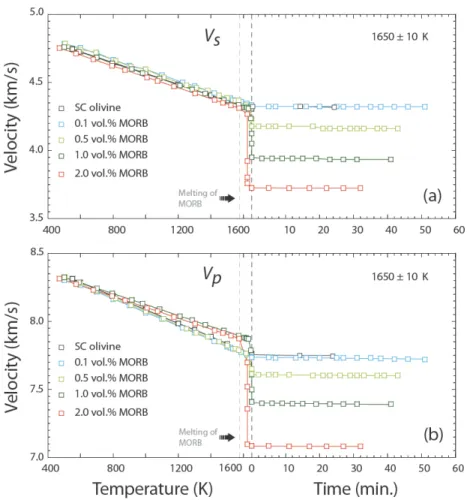
165
affected by the stress field and the temperature distribution within the sample and it is highly
166
unlikely that two experiments would yield identical melt distributions.
167
In this study, we aim to investigate the effect of ongoing textural modification of partially
168
molten peridotite analog on both electrical conductivity and sound wave velocity. Here we have
169
developed a novel high-pressure multi-anvil cell design to investigate simultaneously the seismic
170
and electrical properties of partially molten samples. Acoustic wave velocity (Vp and Vs) and EC
171
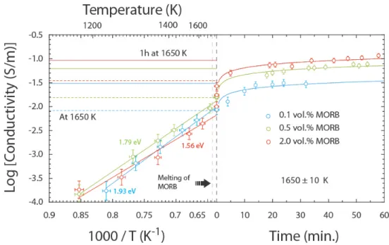
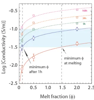
are measured on an identical sample presenting the same temperature gradient, stress field and
172
the chemical impurities, which all influence the melt content and the melt texture in partially
173
molten high pressure samples. This critical improvement enables us to compare the seismic and
174
electrical responses to the onset of melting, to different melt volume fractions and to the
175
evolution of melt interconnectivity of a partially molten sample. Based on our observations, we
176
suggest possible scenario which may resolve the observed discrepancy of melt fraction
177
estimations based on EC and SV measurements.
178 179
2. Methods 180
2.1 Sample preparation 181
Samples used in this study were a powder mixture of natural San Carlos (SC) olivine and
182
volatile-rich natural MORB glass (location 6°44’N, 102°36’W, collected during the Searise-1
183
research cruise). The volatile content is estimated to be 2730 (±140) ppm wt. H2O and 165 (±40)
184
ppm wt. CO2 [Andrault et al., 2014], comparable with the average H2O and CO2 levels observed
185
in MORB from diverse geological settings [Naumov et al., 2014]. The MORB glass and
186
inclusion free, hand-picked, SC olivine crystals were crushed separately and reduced to fine
187
grain powders (see grain size distribution in figure S1). The water content analysis of the San
188
Carlos olivine indicates less than 1 wt. ppm of water [Soustelle and Manthilake, 2017]. These
189
powders were then mixed in predetermined weight proportions to obtain the desired melt
190
fractions at high temperature. The accurate determination of melt fraction using the image
191
analysis is an uncertain exercise. The mixing of MORB with olivine results in an accurate
192
control of the melt fraction in the sample as the MORB component melts instantaneously above
193
its melting temperature, which is significantly lower than the olivine solidus. This procedure has
194
been extensively used to obtain a controlled melt fraction in high-pressure experiments [Faul et
195
al., 1994; Cmíral et al., 1998; Maumus et al. 2005; Yoshino et al., 2010; Caricchi et al., 2011;
196
Zhang et al., 2014; Chantel et al., 2016]. While this technique is suitable for obtaining controlled
197
melt fractions (nominal melt fractions) in laboratory experiments, it cannot be used as a
198
substitute for the physical property measurements of incipient melting scenarios [Sifré et al.,
199
2014]. We prepared different starting materials with MORB volume fractions of 0.1, 0.5, 1 and 2
200
vol. % mixed with San Carlos olivine. The powder mixtures were ground with an automatic
201
agate mortar for more than 2 hours to obtain a homogeneous distribution of the MORB
component. The starting powder average grain size was estimated to be 3.74 ± 3.32 µm (Fig.
203
S1). In order to achieve high accuracy during weighting the powder, we prepare more than 5 g
204
for each composition. The resulting powder mixtures were then hot pressed at 2.5 GPa and 1100
205
K for 2 hours using a 1500 ton multi-anvil apparatus. The low temperature for hot pressing
206
experiments (below the melting temperature of MORB) ensures that the starting materials are
207
melt free and thus that the evolution of melt texture occurs during the conductivity and velocity
208
measurements.
209 210
2.2 High-pressure high-temperature experiments 211
High-pressure, high-temperature experiments were performed using a 1500 ton
Kawai-212
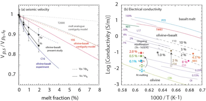
type multi-anvil apparatus at Laboratoire Magmas et Volcans, Clermont-Ferrand, France. For
213
experiments conducted at 2.5 GPa, we used octahedral pressure media composed of MgO and
214
Cr2O3 (5 wt. %) in an 18/11 multi-anvil configuration (octahedron edge length / anvil truncation
215
edge length) (Fig. 1). The assembly was designed to accommodate the geometrical requirements
216
for measurements of Vp, Vs and EC in a single high pressure cell. The pre-synthesized
217
cylindrical sample was inserted into a hexagonal boron nitride (hBN) capsule. The use of
high-218
purity hBN sintered at high temperature and pressure without binder (Type - BN HP, FINAL
219
Advanced Materials) prevents the B2O3 reacting with the silicate melt. The hBN capsule also
220
helps to electrically insulate the sample with respect to the furnace. The furnace is composed of a
221
50 μm thick cylindrical Re foil, with apertures for the electrode and the thermocouples wires. A
222
zirconia sleeve was placed around the furnace to act as a thermal insulator. Oxygen fugacity of
223
the sample was not controlled during the experiments, but should be below Re-ReO2 buffer.
We placed two electrodes made of Re discs (25 µm thick) at the top and bottom of the
225
cylindrical sample. A tungsten-rhenium (W95Re5-W74Re26) thermocouple junction was placed at
226
one end of the sample to monitor the temperature. On the opposite side it was connected to a
227
single W95Re5 wire (See Fig. S2 for details on electrode connection). We collected impedance
228
spectra between the two W95Re5 wires. Cylindrical MgO ceramic sleeves were used to insulate
229
the electrode wires from the furnace. A dense Al2O3 buffer rod was placed between one of the
230
tungsten carbide (WC) anvil truncations and the sample to enhance the propagation of elastic
231
waves and to provide sufficient impedance contrast to reflect ultrasonic waves at the buffer
rod-232
sample interface. Both ends of the anvil, the alumina buffer rod and the samples were mirror
233
polished using 0.25 μm diamond pastes in order to enhance mechanical contacts. All ceramic
234
parts of the cell assembly, including the pressure media, were fired at 1373 K prior to the
235
assembling in order to remove any absorbed moisture.
236 237
2.3 Acoustic wave velocity measurements 238
Acoustic wave velocities of samples were measured using the ultrasonic interferometry
239
technique [Chantel et al., 2016]. In this method, electrical sine wave signals of 20–50 MHz (3–5
240
cycles) with Vpeak-to-peak of 1–5 V were generated by an arbitrary waveform generator (Tektronix 241
AFG3101C) and were converted to primary (VP) and secondary (VS) waves by a 10° Y-cut 242
LiNbO3 piezoelectric transducer attached to the mirror polished truncated corner of a WC anvil.
243
The resonant frequency of the transducer is 50 MHz for compressional waves (P-waves) and 30
244
MHz for shear waves (S-waves). Elastic waves propagated through the anvil, the alumina buffer
245
rod (BR) and the samples, and were reflected back at the anvil-BR, BR-sample, and
sample-246
electrode interfaces. We also consider possible reflections from the Re electrodes [Davies and
O'Connell, 1977; Jackson et al., 1981; Niesler and Jackson, 1989] (Text S1 c). The reflected
248
elastic waves were converted back to electrical signals by the transducer and captured by a
249
Tektronix DPO 5140 Digital Phosphor Oscilloscope at a rate of 5 × 10⁹ sample/s. Signals at 20,
250
30, 40 and 50 MHz were recorded at each temperature step. The two-way travel time for the
251
acoustic waves propagating through the sample can be determined by the time difference
252
between the arrivals of the echoes from the BR-sample interface and the sample-electrode
253
interface by the pulse-echo overlap method [Kono et al., 2012].
254 255
2.4 Electrical conductivity measurements 256
EC measurements were performed using the ModuLab MTS Impedance/Gain-phase
257
analyzer in the frequency range of 106 - 101 Hz. Polyphasic samples are characterized by a
258
combination of resister-capacitor/constant phase element (R-C/CPE) circuits and the resistance
259
can be obtained by fitting the impedance spectra to appropriate equivalent circuits (Fig. S3).
260
Once the sample resistance has been determined, conductivity can be calculated using the sample
261
dimensions determined at each temperature using the thermal expansion of the constituent
262
phases. The insulation resistance of the assembly was determined in a preliminary experiment
263
using an hBN rod at similar pressure-temperature conditions and was observed to be lower than
264
the sample resistance.
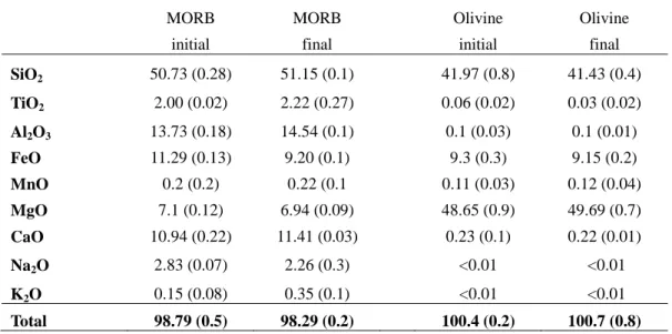
265
At the target pressure of 2.5 GPa, the sample was kept at 500 K for more than 12 hours.
266
While maintaining 500 K, the electrical resistance of the samples, measured at regular intervals,
267
usually increases due to the removal of the moisture absorbed by the sample and surrounding
268
materials. This step is crucial to prevent the moisture (H2O) being incorporated into the sample at
269
higher temperatures [Manthilake et al., 2009]. The next heating cycle started once the resistance
reached a steady value, which is often 1-2 orders of magnitude higher than the resistance
271
measured at the beginning of the heating cycle. We generally performed several heating-cooling
272
cycles at temperature steps of 50-100 K, until sample resistance was reproducible between the
273
heating and cooling paths. This procedure minimizes the uncertainty of EC measurements due to
274
impurities (H2O and CO2). Once the solid sample EC was reproducible (without moisture), the
275
temperature was gradually increased in smaller temperature steps (25 K) to initiate melting.
276
Sample melting is characterized by a drastic decrease in the sample resistance (increase in
277
conductivity). Finally, the temperature was kept constant at 1650 K and impedance spectra were
278
collected at regular intervals for more than 1 hour.
279 280
2.5 Melt textures and dihedral angle measurements 281
Micro-textures of the recovered samples were investigated with a Field Emission Gun
282
Scanning Electron Microscope (FEG-SEM) with an accelerating voltage of 15 kV and working
283
distance of 9 - 11.6 mm. High magnification back scattered electron (BSE) images were obtained
284
in order to identify the degree of interconnectivity and the structure of the melt at the grain
285
boundaries in partially molten samples after SV and EC measurements. The presence of the hard
286
alumina piston may introduce differential stresses to the sample, resulting in a shape-preferred
287
orientation (SPO) in partially molten samples [Bussod and Christie, 1991]. To characterize the
288
possible melt alignment in an olivine matrix, we performed image analyses on BSE images along
289
a section parallel to the axis of the cylindrical sample. The orientation of the long axis of melt
290
pockets and area of the melt pockets were obtained by image processing techniques using Matlab
291
software (Fig. S4).
292 293
2.6 Grain size and grain orientation distribution 294
The grain size of our samples was estimated using two different techniques: the intercept
295
method, and using FOAMS software [Shea et al., 2010]. The intercept method estimates the
296
number of intersections of grain boundaries with a random line drawn across the sample. The
297
length of the line is important in order to statistically cross enough grains. The FOAMS software
298
measures every isolated particle from skeletonized images and estimates its morphological
299
parameters: area, perimeter, shape from 2D ellipse with a long and short axis, etc. The program
300
also calculates 2D parameters such as aspect ratio and elongations. From the binary images, the
301
code can convert 2D morphological information into 3D information using the equivalent
302
diameter for spherical geometry by means of stereological conversion equations from [Sahagian
303
and Proussevitch, 1998]. This program works properly for all type of samples for 2D
304
information. Volumetric estimations (2D to 3D) can be performed when the grains are mostly
305
rounded and do not show strongly elongated shapes. Results are given in table S1.
306 307
2.7 Experimental uncertainties 308
Experimental measurements of Vp, Vs and EC are subjected to uncertainties originating
309
from the estimation of temperature pressure, sample dimensions and fitting errors. Errors have
310
been estimated to be 2.5 % for seismic velocities (2σ), 5 % for velocities drops (2σ) and 5 % for
311
EC values (2σ). Errors on the melt fractions are less than 1% relative (ex: 1±0.01 % of MORB).
312
Detailed sources of uncertainties for each technique and error propagation calculations are given
313
in supporting information (Text S1) [Bouhifd et al., 1996; Gillet et al., 1991; Li et al., 2007].
314
Error bars are reported in each figure when larger than the symbol size except figure 4 and 8a)
315
for visibility.
3. Results 318
3.1 Acoustic velocity 319
The acoustic wave velocities obtained for samples containing SC olivine and 0.1, 0.5, 1
320
and 2 % nominal volume fractions of melt are shown in figure 2. Below the melting temperature,
321
Vp and Vs decrease with increasing temperature, emphasizing the characteristic decrease of bulk
322
and shear modules with temperature. Upon melting of the MORB component, which is at about
323
1590 K, both Vp and Vs decrease significantly for the samples with 0.5 to 2 % MORB. The
324
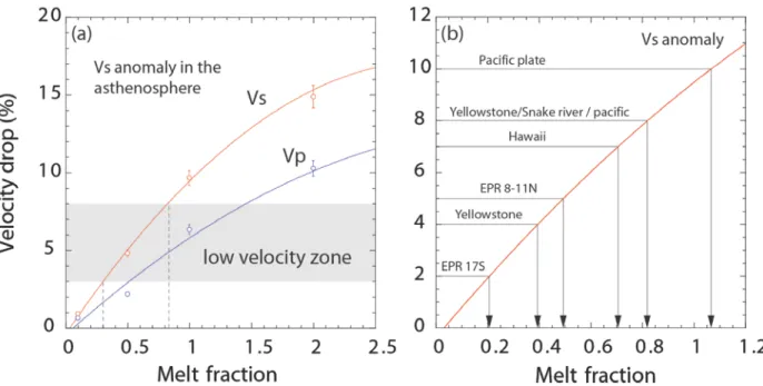
magnitude of the velocity drop is positively correlated to the MORB fraction in the sample, but
325
no significant change is observed at the melting temperature for pure olivine and the sample with
326
0.1 vol. % melt. After the initial decrease in response to the MORB melting, the acoustic
327
velocities Vp and Vs remain unchanged while maintaining the sample at a constant temperature
328 of 1650 K. 329 330 3.2 Electrical conductivity 331
The electrical conductivity of samples containing 0.1, 0.5 and 2 vol. % of nominal melt
332
fractions are shown in figure 3. At the melting temperature of MORB (~1590 K), the samples
333
with 0.5 to 2 vol. % melt indicate sudden increases in conductivity (up to a factor of 5),
334
compared to their solid counterparts. However, no immediate change in conductivity is observed
335
for 0.1 vol. % melt upon crossing the temperature threshold. EC of all melt-bearing samples
336
continues to increase after the melting event, while being kept at a constant temperature of 1650
337
K. The rate of increase of conductivity gradually decreases with time (Fig. 3), probably
338
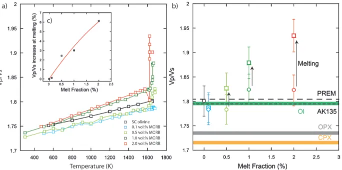
approaching a steady-state with time, however these 1h duration experiments didn’t reached a
339
stable EC value over time. The conductivity values after being kept at 1650 K for more than 30
minutes indicate an increase in conductivity of 0.6 log units, a factor of 3.98, for the 0.1 % melt
341
sample compare to the value obtained before melting. The conductivity variations after being
342
kept for more than 50 minutes at 1650 K, are about 0.6 log units, a factor of 3.98, for the 0.5 %,
343
and a 0.4 log units, a factor of 2.51, for the 2 % melt-bearing samples.
344 345
3.3 Textural analyses of samples and melt 346
The presence of melt is clearly visible for all samples, with melt distributing along the
347
grains boundaries as well as triple junction tubes. Interconnected melt networks are visible over a
348
large part of each sample including the samples with 0.1 vol. % of melt (Fig. 4). Using the high
349
resolution SEM images, we determined the wetting angles of the melt-solid interfaces, which
350
indicate a median angle of 27 ± 4º.
351
Table S1 presents the grain size and grain orientation parameters derived from both
352
intercept and FOAMS software, samples average grain size are similar and between 7 to 15
353
micrometres. The eccentricity is calculated from the best fitting ellipse foci and circle centre.
354
This parameter indicates how far the best fitting ellipse deviates from perfect circularity, the
355
values from 0.76 to 0.84 in our samples indicate that grains are mainly rounded but not perfect
356
spheres. Elongation parameter is expressed by ε = (a-b)⁄(a+b), which characterizes the difference
357
between the long (a) and short (b) axes of the fitting ellipse; large values (close to 1) indicate
358
elongated particles. Our average values trends from 0.25 to 0.36, meaning grains have an elliptic
359
cross section which slightly deviates from circularity. Aspect ratio is expressed as A = b/a, and
360
characterizes the shape of the particle; large aspect ratios (close to 1) indicate particles are
361
rounded and not elongated; our high-intermediate values are good agreement with this
362
observation.
The analyses based on the orientation of the long axis of melt pockets indicate random
364
distribution of melt within the olivine matrix (Fig. S4). The associated histogram indicates no
365
significant preferential orientation.
366 367
4. Discussion. 368
4.1 Effect of evolving melt texture on acoustic wave velocity and electrical conductivity 369
Upon melting, partially molten samples evolve toward textural equilibrium with time,
370
thus improving the melt interconnectivity and melt redistribution within the olivine matrix (Fig.
371
4). The comparison of images of samples before melting and after keeping prolonged time above
372
the melting temperature of MORB clearly demonstrate the evolution of Ol+MORB powder
373
mixture from initial non-equilibrium state (MORB is randomly distributed) to the extensive
374
wetting of crystal faces and the smoothly curved solid-melt interfaces (Fig. S5). The textural
375
equilibrium depends on several factors such as melt fraction, melt chemistry and grain size
376
distribution [Laporte and Provost, 2000]. The melt geometries in olivine-basalt systems consist
377
of grain boundary melt layers, triple junction networks [Yoshino et al., 2005, 2009] and
378
ellipsoïdal discs [Faul et al., 1994]. The continuous increase of EC observed in our experiments
379
can be attributed to the gradual development of an interconnected network of melt channels,
380
which facilitate the movement of charge carried through the melt. In contrast, acoustic wave
381
propagation in a partially molten media should be more affected by the presence of melt in its
382
path (volume fraction), than its fine geometrical evolution subsequent to melt interconnection.
383
We note that the EC increased quickly in the first tens of minutes and showed a flat evolution
384
with almost flat slope after about 1 hour, indicating that the textural modifications that influence
385
the interconnectivity of the melt can be mostly achieved within few hours. The melt takes its
final like shape very quickly (in the first hour), however complete equilibration between melt
387
and host olivine matrix in both chemical and textural aspects require several weeks of annealing
388
[Waff and Blau, 1982; Laporte and Provost, 2000].
389 390
a) Interpretation of acoustic wave velocity results 391
The magnitude of the drop in seismic wave velocity in response to melting is proportional
392
to the melt volume fraction in the sample (Fig. 2). Compared to the higher melt fractions, the
393
sample containing 0.1 % melt does not show abrupt variations of acoustic wave velocity in
394
response to the onset of melting of MORB components. This observation suggests that the
395
volume fraction of melt has to be sufficiently large (higher than 0.1 vol. %) in order to alter the
396
seismic wave propagation through partially molten rock. Also, associated errors to seismic wave
397
velocity measurements and fitting does not allow distinguishing significant drop for low melt
398
fractions (~0.1 %). Further, the relatively constant seismic velocity at a constant temperature of
399
1650 K, after the melting of MORB, suggests that the seismic velocity is less sensitive to the
400
ongoing textural equilibration of the sample. The melt fraction in a partially molten rock with
401
complete wetting properties is observed to be the key parameter controlling the magnitude of
402
seismic velocity in geological systems. The secondary waves (Vs) are more sensitive to the
403
presence of melt due to their near zero shear modulus, which further enhances their ability to
404
detect and quantify melting in laboratory samples.
405
The comparison of present data with previous experimental and theoretical estimations of
406
seismic velocity is shown in figure 5. While our results are consistent with that of [Chantel et al.,
407
2016], there are considerable deviations in our experimental values from those estimated based
408
on theoretical approximations [Takei, 2000]. As explained previously, the disagreement may arise
due to the simplified melt geometries assumed in theoretical models. This observation can be
410
further corroborated by comparing two theoretical models, one based on natural melt geometries
411
[Yoshino et al., 2005], and the other on ideal melt geometries [Takei, 2000]. The model with melt
412
arrangements similar to naturally occurring melt record a significant velocity drop for a given
413
melt fraction compared to the one assuming ideal melt distribution. However, the model based
414
on grain boundary wetness [Yoshino et al., 2005] also predicts the seismic velocities are
415
significantly affected by modifications on the pore geometry. It has been shown that the melt
416
wetting properties vary significantly with increasing pressure and volatile content [Yoshino et al.,
417
2007]. The slight discrepancy between the present study and that of [Yoshino et al., 2005] can be
418
explained by the change in wetting properties, due to improved melt wetting properties at high
419
pressure and the presence of both H2O and CO2 in our samples.
420 421
b) Interpretation of electrical conductivity results 422
The electrical conductivity variation while kept at constant temperature (at 1650 K)
423
provides valuable insights into the development of interconnected melt channels in partially
424
molten samples. For larger melt fractions (above 0.1 %) the melt network forms efficiently as
425
shown by an order of magnitude conductivity increase observed at the onset of melting.
426
However, after the onset of melting and the associated EC jump, while kept at constant
427
temperature of 1650 K, the increase in electrical conductivity for larger melt fractions (2 % with
428
0.4 log unit increase of EC) is smaller than the sample with a low melt fraction (0.1 % with 0.6
429
log unit increase of EC). This potentially indicates that when the melt fraction is sufficiently
430
large, the major portion of melt is already arranged into a well distributed network of melt
431
channels. On the other hand, the subsequent modifications improving the melt interconnectivity
have a significant effect on low melt fractions. It has been shown that the melt geometry in a
433
mineral-melt aggregate is determined by the solid-solid and solid–liquid interfacial energies
434
[Laporte and Provost, 2000]. The solid–liquid interfacial energies may control the
435
interconnectivity of a partially molten medium at low melt fraction; the network of melt could be
436
limitedin its 3D extension between the olivine grains, with some surfaces remaining initially
un-437
wetted due to surface tension.
438
As for acoustic velocity, a sharp variation in electrical conductivity was not immediately
439
apparent for the sample with 0.1 % melt fraction. However, when maintained at 1650 K, EC
440
continued to increase for the 0.1 % melt sample, after 1h to 0.6 log unit higher than the
441
conductivity of the sample before melting. This observation suggests that the electrical
442
conductivity method can be used to detect melt fractions lower than 0.1 % as long as the
443
measurements are performed on texturally equilibrated samples. As well, EC is very sensitive to
444
the onset of melting with few orders of magnitude of increase after only few minutes. Reading
445
value of sample resistance (direct measurement to infer EC) is instantaneous and can be a
446
powerful tool to detect the onset of melting during an experiment.
447
The electrical conductivity of similar olivine-basalt systems has been investigated in
448
previous experiments [Maumus et al,. 2005, Yoshino et al., 2010; Caricchi et al., 2011; Zhang et
449
al., 2014, Laumonier et al., 2017] (Fig. 5). While measured conductivities are located within the
450
individual EC measurements of olivine [Constable, 2006, Laumonier et al., 2017] and basaltic
451
melt [Presnall et al., 1972; Tyburczy and Waff, 1983; Ni et al., 2011, Laumonier et al., 2017], the
452
partially molten systems do not display good agreement between different studies. The slightly
453
higher EC observed for partially molten samples in [Yoshino et al., 2010], compared to our study
454
may have been due to their use of texturally equilibrated melt-bearing samples (pre-synthesized
samples in a piston cylinder apparatus) in electrical conductivity measurements, which compare
456
favourably with our observations. Values comparable to “equilibrated samples” conductivities
457
can be retrieved, by using extrapolation of our EC versus time trend, for timescales of days or
458
weeks, indicating full equilibration might require might require a significant time (Fig. 5 and 6).
459
This again, underlines the crucial importance of the use of equilibrated EC values for safe
460
comparisons.
461
4.3 The source of discrepancy 462
The interpretation of seismic and electrical anomalies in terms of melt fraction often
463
results in conflicting estimations as to the extent of melting in the asthenosphere [Pommier and
464
Garnero, 2014; Karato, 2014]. A conductivity model based on major element chemistry of melt
465
attributed the apparent inconsistencies in conductivity measurements to possible chemical
466
variations in the melt [Pommier and Garnero 2014]. Their model predicts that low degree
467
melting of peridotite produces melt that is more conductive than basaltic compositions. We find
468
their approach is an important step towards unifying the seismic and electrical observations.
469
However, the melt fractions estimations used in their study were based on theoretical models,
470
which appear to underestimate the effect of melt fraction on seismic velocity.
471
Monitoring the behaviour of melt-bearing samples for an extended period of time at high
472
pressure and high temperature remains a challenging exercise. Escape of melt during prolonged
473
heating is one of the major sources of failure, and experimental studies often overcome this issue
474
by shortening the duration of the in situ measurements at high temperature. However, our results
475
demonstrate that the EC values can vary significantly with time within the first hour of
476
measurements, and relatively stable EC values can be obtained once the 3D interconnected
477
network has been established. Texturally non-equilibrium melt can lead to an underestimation of
the total effect on EC of a given melt fraction (Fig. 6). Comparison of such measurements with
479
geophysical profiles, therefore, results in an overestimation of the melt fraction in the
480
corresponding region in the Earth’s mantle. Values here provided after 1 h at 1650 K are not fully
481
stabilized as highlighted by the subtle slope of the fit. We also note that once the sample
482
conductivity stabilized, as a result of improved melt interconnectivity, electrical conductivity
483
values of samples containing 0.1, 0.5 and 2 % are not considerably different (less than one order
484
of magnitude). This difference becomes subtle, close to the uncertainty of measurements, for
485
higher melt fractions according to the trend shown in figure 6. This implies that uncertainties on
486
inferred melt fractions from EC can be very important if implied melt fractions are higher than
487
few percents. This observation is particularly crucial for magnetotelluric (MT) profiles with low
488
spatial resolution. For these reasons, EC values here provided will not be further used for
489
geophysical implications. However, we note that the electrical conductivity measurements are
490
superior over acoustic wave velocity for detecting low melt volume fractions for samples with
491
evolved melt textures. If the wetting properties of the melt are modified by the presence of
492
significant amounts of volatiles in the melt (H2O and CO2) the electrical response for low melt
493
fractions is instantaneous [Sifré et al., 2014].
494
In this study, we observe real-time Vp, Vs and EC responses during melting and
495
consecutive textural evolution of melt. The variation of electrical conductivity subsequent to the
496
melting of MORB can also be caused by the chemical changes occurring at high temperatures for
497
a prolonged period of time. The effect of change in chemical composition on electrical
498
conductivity in melt has been investigated in previous studies [Roberts and Tyburczy, 1999], with
499
a general trend showing an increase in conductivity with increasing alkali and Fe+Mg contents
500
and a decrease with increasing silica content. However, we observe that the melt composition
stays similar to the starting MORB composition during the experiments, except for a minor
502
decrease in Fe content (Table 1). The Na is an important charge carrier in silicate melt [Pfeiffer,
503
1998; Gaillard and Iacono-Marziano, 2005; Ni et al., 2011] and Na contents in our melt remains
504
similar to the starting composition. Based on the totals of chemical analyses of melt, we confirm
505
that significant volatile enrichments may not occur in our melt. Therefore, the observed
506
conductivity increase with time is not expected to be caused by any chemical modification to the
507
melt. This observation also confirms that the final melt fraction in the sample stays similar to the
508
starting material. Similarly, due to the low partition coefficient between olivine and melt
509
(~0.004) [Novella et al., 2014], the water is mostly retained by the melt phase, so proton (H+)
510
diffusion in olivine affecting the electrical conductivity at high temperature can also be ruled out.
511
The constant velocity after the melting of MORB components also rules out the possible increase
512
in melt fraction in the sample at constant temperature, which is also supported by image analysis
513
and chemical mapping of the sample. Further, analyses on the orientation of the matrix and melt
514
pockets in our samples indicate random shape preferred orientation (SPO) ruling out melt
515
channelling due to possible anhydrostaticity in the high-pressure cell assembly (Fig. S4).
516 517
4.4 Applications of laboratory results to the Earth's interior 518
The comparison between laboratory data and seismological signals requires experiments
519
in which the molten phase is in textural equilibrium with the solid matrix. Due to time-limited
520
laboratory experiments, transient conditions may affect the results of acoustic velocities. In this
521
case, textural analysis is important for correct interpretation of experimental data and run
522
products. In a partially molten system at given pressure and temperature, the melt network can
523
evolve to minimize the energy of melt-solid interfaces. This equilibration process concerns the
wetting angle θ at solid-solid-melt triple junctions, the area-to-volume ratio of melt pockets at
525
grain corners and the melt permeability threshold [Laporte et al., 1997]. The small dihedral
526
angles estimated for our partially molten samples ensures complete grain boundary wetting and
527
melt interconnectivity even for extremely low melt volume fractions [von Bargen and Waff,
528
1986; Laporte et al., 1997; Laporte and Provost, 2000], which is crucial for propagation of
529
seismic waves. The solid-melt dihedral angle is known to vary with pressure, temperature and
530
with the composition of the melt phase [Minarik and Watson, 1995; Yoshino et al., 2005].
531
Experimental studies suggest that textural equilibration is a time-dependent process, which
532
usually requires long annealing times (weeks or months) [Waff and Blau, 1982; Laporte and
533
Provost, 2000, Maumus et al., 2005]. Still, small dihedral angle (10-30°), the extensive wetting
534
of crystal faces and the smoothly curved solid-melt interfaces observed in our samples are strong
535
indications that the microstructure has reached transient conditions and forming a melt solid
536
network close to equilibrium textures [Cooper and Kohlstedt, 1984; Waff and Faul, 1992;
537
Cmíral et al., 1998] (Fig.4). Further, after reaching the peak temperature, the acoustic velocity
538
remains nearly constant (Fig. 2), suggesting that the samples are well relaxed, enabling a safe
539
comparison of our seismic wave velocity measurements with geophysical observations.
540
In addition, the extrapolation of laboratory acoustic wave velocities measurements to
541
natural observations require the consideration of both anelasticity and frequency effects.
542
Laboratory experiments (when not torsional) are usually performed at the frequency range from
543
20 to 50 MHz. The choice of this frequency range is determined by both requirements on
544
excitation frequencies for the piezo-electric transducer as well with the restricted size of the
545
probed samples in HP-HT apparatus.
Both anelasticity and anharmonicity that are accounting for the temperature dependence
547
of sound velocity could lower the observed velocities. These are functions of frequency,
548
temperature, pressure, mineral/melt intrinsic properties (including the chemical composition) as
549
well as grain-size and grain boundaries micro textures [Rivers and Carmichael, 1987; Karato,
550
1993; Jackson et al., 2002, 2004; Faul et al., 2004]. In solids, anharmonic effects related to
551
thermal expansion (∂ρ/∂T) were found to be important in high frequency (MHz) experiments.
552
This process does not imply energy loss and remains nearly insensitive to frequency [Karato,
553
1993]. On the other hand, anelasticity is associated to energy loss and depends on frequency and
554
relaxation effects. Relaxation effects are thermally activated, hence anelasticity must be
555
accounting for a significant part of the attenuation at high temperatures. Anelasticity of partially
556
molten system have been poorly studied [Faul et al., 2004; Jackson et al., 2004]. Because our
557
melt fractions are small (≤ 2 %) and similar to melt fraction estimated in the mantle, the
558
assumption of using anelastic values of pure olivine is reasonable [Jackson et al., 2002; Chantel
559
et al., 2016], also partially molten systems were found to have similar grain boundary sliding
560
process to solid [Jackson et al., 2002; Faul et al., 2004]. Nevertheless, this process is more easily
561
activated in melt bearing samples, where weaker grain boundaries have been reported [Faul et
562
al., 2004]. In addition, most of silicate melts have very high absorption in this frequency range
563
and signals are seriously attenuated [Rivers and Carmichael, 1987]. However, this study showed
564
that the echo overlap technique is suitable for high-Q melts, and thus appropriate for MORB
565
melts. This study also stressed that for low viscosity melts (<1000 Pa.s), which is the case of
566
MORB melts at high temperature (presence of volatiles will significantly increase this effects),
567
velocities are independent from frequency, as expected when wave’s period is much smaller than
568
the characteristic relaxation time (1/f << τ). Relaxation time was estimated using the relation τ =
0.01*η*β, where β is the inverse of adiabatic compressibility and η the melt viscosity, used for
570
fitting of theoretical and experimental dispersion curves by Rivers and Carmichael, (1987).
571
Calculation using their parameters for the Kilauea basalt (1700 K) yields relaxation time of 0.467
572
nanoseconds for frequency of 30 MHz (used in our study). The product of angular frequency by
573
relaxation time between 10-2 and 10-1 (0.088) can be converted into a C/C0 ratio (see fig 10
574
therein). It estimates the measured velocity to be similar to the relaxed one as the ratio is very
575
close to unity (1 ≤ C/C0 < 1.10), pointing a very small effect of anelastic behavior. Our
576
moderately hydrous MORB probably have a lower viscosity and accordingly a shorter relaxation
577
time favoring our conclusions.
578
Detailed discussion on quality factor (Q) estimation by ultrasonic experiments, on
579
similar compositions, has already been made by Chantel et al., (2016). However, our ∂ln(Vp)/∂T
580
and ∂ln(Vs)/∂T values of -4.95 and -8.78 (*10-5
) K-1, of our olivine + MORB samples prior
581
melting, are somewhat similar with temperature dependence values calculated by high Q from
582
Karato, (1993), indicating a good agreement with pure olivine data up to melting point with
583
anharmonic plus anelastic behavior.
584
Finally, the use of MHz frequencies tends to underestimate the effect of anelasticity. This
585
increases our uncertainty on our measurements, but this uncertainty must be reasonable as shown
586
by the small errors estimated in absorption calculations (4%) [Rivers and Carmichael, 1987], as
587
well with near relaxed sound speed found for melt. In this study, we thus report a minimal effect
588
of the presence of partial melt on the acoustic wave velocities and consider similar bias as
589
estimated for solids (anelasticity and anharmonicity) because small fraction of melt seems to
590
have only a moderate effect. Our extrapolation suffers also from grain size considerations as
detailed by Jackson et al. (2002), even though this process was found to be nearly frequency
592
independent for attenuation at mantleconditions.
593 594
4.5 Geophysical implications 595
Our study demonstrates that the melt content in a partially molten media can be better
596
quantified by using the reduction of seismic velocity for melt fractions with a minimum
597
detectable melt fraction between 0.5 % and 0.1 % (no seismic velocity drop seen for 0.1 %). On
598
the other hand, for the studied melt fractions of 0.1-2.0 % with well-developed interconnectivity,
599
electrical conductivity, varies within a strict range of about 0.5 log units even if transient values
600
were only reached, too narrow to resolve fine melt structures without introducing significant
601
uncertainties.
602
In this study, we specifically use the % drop in acoustic wave velocity as a measure to
603
determine the melt fraction. Our study indicates that the 3-8 % global reduction in seismic
604
velocity (Vs) observed at the top of the asthenosphere [Anderson and Sammis, 1970; Widmer et
605
al., 1991; Romanowicz, 1995] can be explained by 0.3-0.8 % volatile-bearing melt (Fig. 7a).
606
However, these values may vary laterally depending on the extent of melting at the
607
corresponding temperatures and the volatile contents in the mantle [Sifré et al., 2014]. Regional
608
Vs variations of up to 10 % observed below the Pacific plate [Schmerr, 2012] indicate large melt
609
fractions of up to 1 % present in some parts of the asthenosphere, suggesting large
610
heterogeneities in terms of melt distribution. Apart from the global reduction of seismic velocity,
611
numerous studies report velocity perturbations in various geological settings such as spreading
612
ridges, intraplate mantle plumes and subduction. [e.g. Pommier and Garnero, 2014]. Assuming
613
melt chemistry does not have any significant influence on acoustic wave velocity [Rivers and
Carmichael, 1987]; we compare our melt fraction estimations to those reported using theoretical
615
models (Table S2).
616
In addition to the use of absolute sound wave velocities and velocities drop, the use of
617
Vp/Vs ratio can be of significant interest for comparison with seismological data. Bulk and shear
618
moduli of a partial melt system (a solid containing pore spaces saturated with melt) varies as a
619
function of melt volume fraction. Accordingly, the relative change of Vp/Vs ratio could
620
indicate the presence of melt in deep mantle conditions. As detailed in Chantel et al., 2016, the
621
absolute velocities values measured on analog systems do not compare well with real seismic
622
velocities measurements. It is mainly due to the difference in mineralogy (e.g pure olivine against
623
peridotites) and relaxation effects due to differences in frequencies between natural and
624
experimental seismic velocities estimations (see discussion therein). However, the use of Vp/Vs
625
ratios and its variations allow a relevant comparison of our analog data to natural system as
626
changes are relative and not based on absolute velocities values.
627
Our data indicate that below melting point, Vp/Vs ratio increases from 1.75 to 1.8 from
628
room temperature up to 1650 K (Fig. 8). These values are consistent with values observed for
629
solid upper mantle ranging from 1.7 to 1.8 given by standard models such as PREM [Dziewonski
630
and Anderson, 1981] or AK135 [Kennett et al., 1995]. These values are also consistent with
631
moderate Vp/Vs values obtained from upper mantle minerals, ranging also between 1.7 and 1.8
632
for olivine (1.8), clino and othropyroxenes (1.72 and 1.74) at the same pressures [Li and
633
Liebermann, 2007]. At melting, we observe a strong and sudden increase of the Vp/Vs ratio. The
634
magnitude of the increase correlates positively with the melt fraction. Vp/Vs ratios above 1.9 are
635
observed for sample with 2% melt fraction (Fig. 8 c). Our Vp/Vs ratio values compare favorably
636
with LVZ estimations with ratios given by global models ranging between 1.8 and 1.85 and
requiring only moderate amount of melt (<1 % of melt). However, our data implies very high
638
melt fractions involved in local anomalies where Vp/Vs ratios up to 2.5 or more have been
639
reported [Schaeffer et al., 2010, Hansen et al., 2012]. These very high anomalies imply higher
640
melt fractions (12.5 % for Vp/Vs ratio of 2.5, based on the trend defined on Fig. 8 c) even if
641
other physical processes such very high volatiles contents in melts could explain these
642
anomalies.
643
In general, we find that the melt contents reported in previous geophysical studies are
644
consistently higher than the estimations based on laboratory measurements of seismic wave
645
velocities. The majority of these studies used the theoretical prediction of velocity reduction for
646
partially molten rocks, which underestimate the effect of melt fraction on seismic velocity. The
647
use of our laboratory measurements provides melt fractions that are consistent with petrological
648
models. Further, we believe that the refined melt fraction estimations would provide a solid
649
platform to constrain a meaningful cross correlation between field-based seismic and electrical
650
observations. The effect of the chemical composition of melt on acoustic wave velocity is one of
651
the important aspects worth exploring in future studies.
652 653
5. Conclusions 654
This study presents the first simultaneous measurements of electrical conductivity and
655
acoustic wave velocity of partially molten samples of geophysical importance. The results
656
highlight how electrical conductivity and acoustic wave velocity respond to the evolving melt
657
texture from a completely random melt distribution. The continuous increase of electrical
658
conductivity at constant temperature, after melting of MORB, indicates that the melt
659
interconnectivity evolves with time. In contrast, constant seismic velocity after the melting
suggests acoustic velocity is sensitive to the melt volume fraction in the sample, but less affected
661
by the evolving melt texture. Our results suggest that the electrical conductivity of partially
662
molten materials measured before reaching the evolved melt interconnectivity can lead to an
663
underestimation of the EC for a given melt fraction. This may result in an over-estimation of
664
melt fraction in geological settings. Overall, the Vs measurements appear to be a more
665
appropriate method for determining the melt fraction in a partially molten system with complete
666
wetting properties. The previous approximations based on theoretical models of seismic velocity
667
appear to overestimate the extent of melting in the mantle. This study demonstrates the necessity
668
of using electrical conductivity values from texturally equilibrated partially molten sample for
669
comparison with geophysical data.
670
Acknowledgments 671
We thank J-M Henot for the SEM analyses, J-L Devidal for the electron microprobe
672
analyses and A. Mathieu for the technical assistance. We thank F. Gaillard for beneficial
673
discussions. DF acknowledges S Thivet for FOAMS assistance and starting powder analysis.
674
GM acknowledges funding from the French PNP program (INSU-CNRS) and Actions initiatives
675
OPGC 2014. DA is supported by ANR-13-BS06-0008. This research was financed by the French
676
Government Laboratory of Excellence initiative n°ANR-10-LABX-0006, the Région Auvergne
677
and the European Regional Development Fund. This is Laboratory of Excellence ClerVolc
678
contribution number xx. All of the experimental data and numerical modelling are provided in
679
the figures and tables obtained by methods described in the text.
680 681
References 682
Anderson, D., and C. Sammis (1970), Partial melting in the upper mantle, Phys. Earth Planet.
683
Inter., 3, 41–50.
684
Andrault, D., G. Pesce, M. A. Bouhifd, N. Bolfan-Casanova, J.-M. Hénot, and M. Mezouar
685
(2014), Melting of subducted basalt at the core-mantle boundary., Science, 344(6186), 892–
686
5, doi:10.1126/science.1250466.
687
Bouhifd, M.A., D. Andrault, G. Fiquet and P. Richet (1996), Thermal expension of forsterite up
688
to the melting point, Geophysical Research Letters,23: 1143-1146.
689
Bussod, G. Y., and J. M. Christie (1991), Textural Development and Melt Topology in Spinel
690
Lherzolite Experimentally Deformed at Hypersolidus Conditions, J. Petrol., 17–39.
691
Caricchi, L., F. Gaillard, J. Mecklenburgh, and E. Le Trong (2011), Experimental determination
692
of electrical conductivity during deformation of melt-bearing olivine aggregates:
693
Implications for electrical anisotropy in the oceanic low velocity zone, Earth Planet. Sci.
694
Lett., 302(1–2), 81–94, doi:10.1016/j.epsl.2010.11.041.
695
Cartigny, P., F. Pineau, C. Aubaud, and M. Javoy (2008), Towards a consistent mantle carbon
696
flux estimate: Insights from volatile systematics (H2O/Ce, δD, CO2/Nb) in the North
697
Atlantic mantle (14° N and 34° N), Earth Planet. Sci. Lett., 265(3–4), 672–685,
698
doi:10.1016/j.epsl.2007.11.011.
699
Chantel, J., G. Manthilake, D. Andrault, D. Novella, T. Yu, and Y. Wang (2016), Experimental
700
evidence supports mantle partial melting in the asthenosphere, Sci. Adv., 2(5), e1600246,
701
doi:10.1126/sciadv.1600246.
702
Cmíral, M., J. D. Fitz Gerald, U. H. Faul, and D. H. Green (1998), A close look at dihedral
703
angles and melt geometry in olivine-basalt aggregates: A TEM study, Contrib. to Mineral.