A constitutive theory for the mechanical response of
amorphous metals at high temperatures spanning the
glass transition temperature: application to microscale
thermoplastic forming of Zr
4
1.
2
Til
3.
8Cu12.
5Ni10Be
22.
5
by
David Lee Henann
B.S., State University of New York at Binghamton (2006)
Submitted to the Department of Mechanical Engineering
in partial fulfillment of the requirements for the degree of
Master of Science
at the
Massachusetts Institute of Technology
May 2008
@
Massachusetts Institute of Technology 2008. All rights reserved.
Author ... .. ... ... .-
.
.,...
I...
Department of Mechanical Engineering
May 9, 2008
Certified by ... :../ ... ...
Lallit Anand
Professor of Mechanical Engineering
/•,lhesis Supervisor
Accept d by.
...
Chairman, Department Committee on Gra
JUL 2 9 2008
LIBRARIPQ.
Lallit Anand
Lduate Students
A constitutive theory for the mechanical response of amorphous
metals at high temperatures spanning the glass transition
temperature: application to microscale thermoplastic forming of
Zr
41.
2Ti
13.8Cu
12.
5Ni
10Be
22.5
by
David Lee Henann
Submitted to the Department of Mechanical Engineering
on May 9, 2008, in partial fulfillment of the
requirements for the degree of
Master of Science
Abstract
Bulk metallic glasses (BMGs) are a promising emerging engineering material distinguished
by their unique mechanical properties and amorphous microstructure. In recent years, an
ex-tremely promising microscale processing method for bulk metallic glasses, called
thermoplastic-forming has emerged. As with any emerging technology, the scientific basis for this process
is at present fragmented and limited. As a result their is no generally agreed upon
the-ory to model the large-deformation, elastic-visco-plastic response of amorphous metals in
the temperature range relevant to thermoplastic-forming. What is needed is a unified
con-stitutive framework that is capable of capturing the transition from a elastic-visco-plastic
solid-like response below the glass transition to a Newtonian fluid-like response above the
glass transition.
We have developed a finite-deformation constitutive theory aimed to fill this need. The
material parameters appearing in the theory have been determined to reproduce the
ex-perimentally measured stress-strain response of Zr
41.
2Ti:
3.sCUl
2.
5Ni10Be
22.
5(Vitreloy-1) in a
strain rate range of [10
- 5, 10-1] s
-1, and in a temperature range [593, 683] K, which spans the
glass transition temperature 0,
=
623K of this material. We have implemented our theory
in the finite element program ABAQUS/Explicit. The numerical simulation capability of
the theory is demonstrated with simulations of micron-scale hot-embossing processes for the
manufacture of micro-patterned surfaces.
Thesis Supervisor: Lallit Anand
5
Acknowledgments
First, I would like to thank my advisor Lallit Anand for his support. Under his guidance,
I have learned not only a great deal about mechanics and materials but also how to think
like a successful researcher. His encouragement to think creatively and push the envelop will
continue to be an inspiration throughout my career.
My labmates, as well as the extended mechanics and materials group, have been like a
second family. I would particularly like to thank Vikas Srivastava and Shawn Chester for
many fruitful discussions, both relevant and irrelevant to our work. Furthermore, I would
like to thank Shawn for his various technical assistance and acknowledge that his help comes
faster than both the internet and email. An additional thanks to Ray Hardin for his help
with various administrative issues, as well as his interest in my musical pursuits.
My roommates Jordan and Andrew have been like yet another family to me and have
helped me to maintain some semblance of balance in my life over the last few years. I would
also like to thank my girlfriend Stephanie for her support and her ability to bring out the
best in life.
Of course, I thank my actual family, particularly my parents, for their constant
encour-agement and interest.
Financial support for this research was provided by grants from the NSF (CMS-0555614)
and the Singapore-MIT Alliance (MST).
And lastly, I dedicate this thesis to my dog, Emily, who passed away during its writing.
She brought my family and me many years of happiness and will be fondly remembered.
Contents
List of Figures
9
List of Tables
11
1 Introduction
13
Bibliography
...
....
...
... . .
...
16
2 Finite-deformation Theory
19
2.1 Introduction ... .... ... 19 2.2 Notation ... .. .... ... ... . 19 2.3 Kinematics ... . .. ... 20 2.3.1 Basic Kinematics ... ... 20 2.4 Frame-indifference ... ... ... ... 222.5 Development of the theory based on the principle of virtual power ... 23
2.5.1 External and internal expenditures of power . ... 23
2.5.2 Principle of virtual power. . ... ... 24
2.5.3 Frame-indifference of the internal power and its consequences .... . 25
2.5.4 Macroscopic force balance. Microscopic force balance ... . 26
2.6 Local dissipation inequality . ... ... 27
2.7 Constitutive theory ... ... 29
2.7.1 Constitutive equations ... ... 30
2.7.2 Thermodynamic restrictions . ... .... 30
2.7.3 Flow rule ... ... ... 31
2.8 Isotropy ... ... 32
2.8.1 Consequences of isotropy of the elastic response . ... 33
2.9 Specialization of the constitutive equations . ... 35
2.9.1 Invertibility assumption for the flow rule . ... 35
2.9.2 Elastic energy and stress . ... ... 35
2.9.3 Kinematical hypothesis for plastic velocity gradient. Internal variables 37 2.9.4 Evolution equations for internal variables. Dilatancy equation . . .. 40
2.10 Summary of the specialized constitutive model . Bibliography
3 Application to amorphous metals at high temperatures
transition temperature
spanning the glass
3.1 Introduction ... 3.2 Internal Friction ...
3.3 Scalar flow function. Evolution of the internal variables . ... 3.3.1 Physical Background ...
3.3.2 The Spaepen model ...
3.3.3 Modified Spaepen model . ... 3.4 Elastic Moduli ...
3.5 Stress-strain response of the metallic glass Zr41.2Ti13.8 CU12.5Ni10Be22 .5
Bibliography
4 Micro-hot-embossing: numerical simulations and experiments
4.1 Introduction ...
4.2 A plain strain micro-hot-embossing . ...
4.2.1
Finite element simulation
4.2.2 Experimental procedures and results ... 4.3 Embossing of a microfluidic mixer device . ...
4.3.1 Finite element simulation ... 4.3.2 Experimental procedures and results ... Bibliography
5 Concluding remarks
5.1 Future Work ...
Bibliography ...
A A heuristic procedure for material parameter
A.1 Introduction .
...
A.2 Estimation of the parameter list MP1 ...
A.3 Estimation of the parameter list MP2 ...
A.4 Estimation of the parameter list MP3 ...
Bibliography .
estimation
B Experimental Details
B.1 Introduction . ... ... B.2 Procedures. ... . . .. ...
B.2.1 Micro-hot-embossing of metallic glass substrates . B.2.2 Micro-hot-embossing of polymeric substrates . . . B.2.3 Temperature Control . ... 95 . . . . 95 ... . 95 . . . . 95 . . . . 96
List of Figures
1-1 A schematic time-temperature-transformation (TTT) diagram for a bulk metal-lic glass ... .. . . . .. ... ... 15 3-1 Stress-strain curves for Vitreloy-1 at various temperatures and strain rates 56 3-2 Stress-strain curves for Vitreloy-1 at various temperatures and strain rates 57 3-3 Stress-strain curves for Vitreloy-1 at various temperatures and strain rates 58 3-4 Stress-strain curves for Vitreloy-1 at various temperatures and strain rates 59 3-5 Stress-strain curves from strain rate decrement and increment experiments for
Vitreloy-1 ... . ... 60 3-6 Stress-strain curves from strain rate decrement and increment experiments for
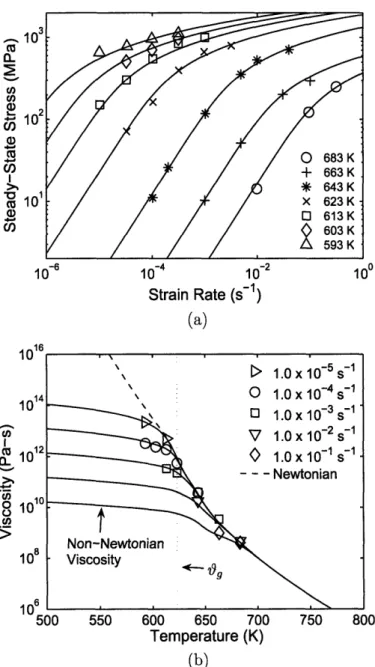
Vitreloy-1 ... ... ... ... 61 3-7 Steady-state stress and viscosity as a function of temperature and strain rate 62 4-1 Plane strain micro-hot-embossing experimental and simulation configurations 70 4-2 Plane strain micro-hot-embossing simulation results . ... . . 71 4-3 SEM results of plane strain micro-hot-embossing experiments ... 72 4-4 Optical profilometry results of plane strain micro-hot-embossing experiments 73 4-5 Microfluidic mixer micro-hot-embossing experimental and simulation
config-urations ... ... ... ... 74 4-6 SEM micrographs of the silicon tool used to emboss a microfluidic mixer pattern 75 4-7 Microfluidic mixer micro-hot-embossing simulation results . ... 76 4-8 SEM results of the micro-hot-embossing of a microfluidic mixer into a metallic
glass substrate ... ... 77 4-9 SEM results of the micro-hot-embossing of a polymeric microfluidic mixer .. 78 A-1 Schematic of the fit of compensated strain rate to
temperature-compensated stress ... . .. .... . ... 90 A-2 Free volume concentration as a function of temperature. . ... . . 90 A-3 Activation energy and activation volume as a function of temperature .... 91 A-4 Dependence of o* on strain rate and temperature. . ... 92 A-5 Temperature dependence of elastic parameters . ... 93
10
B-1 Micro-hot-embossing experimental set-up . ... .. ... . . . 98
B-2 Load train assembly drawing ... ... ... 99
B-3 Platen connector engineering drawing ... ... 100
B-4 Insulating plate engineering drawing . ... ... 101
List of Tables
A.1 Material parameter list 1 ...
A.2 Material parameter list 2 .
...
A.3 Material parameter list 3 .
...
Chapter 1
Introduction
Bulk metallic glasses (BMGs) possess unique mechanical properties which make them
at-tractive materials for fabricating components for a variety of applications. For example, the
commercial Zr-based alloys exhibit superior tensile strength
(-
2.0 GPa), high yield strain
(?
2%), relatively high fracture toughness
(j
10
-
40 MPav/--), and good corrosion resistance
[cf., e.g., 1-3]. A particularly important characteristic of metallic glasses is their intrinsic
homogeneity to the nanoscale because of the absence of grain boundaries. This characteristic,
coupled with their unique mechanical properties, makes them ideal materials for fabricating
micron-scale components, or high-aspect-ratio micro-patterned surfaces, which may in turn
be used, for example, as dies for the manufacture of polymeric microfluidic devices. However,
in order to realize the potential of BMGs in such applications, robust materials-processing
techniques for fabricating microscale features and components must be developed.
In recent years, an extremely promising method called thermoplastic forming has emerged
[cf., e.g., 4-9]. The thermal history of this processing method is schematically shown on a
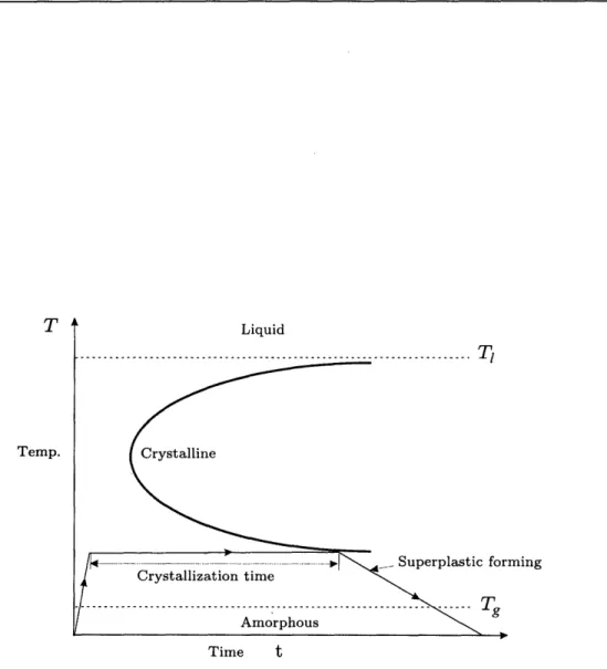
time-temperature-transformation (TTT) diagram for a bulk metallic glass in Figure(I-1). In
this process, the BMG is first obtained in the amorphous state by traditional die-casting.
The shape in this step is not the final shape but in the form of simple plates or rods.
The BMG plate (or rod) is then heated into the supercooled liquid region above the glass
transition temperature of the material, where it may be isothermally formed to produce
intricate microscale patterns and then slowly cooled. Since BMGs in their supercooled
region are metastable, they eventually crystallize; however, the crystallization kinetics in
BMG alloys are sluggish, and this results in a relatively large temperature-time processing
window in which thermoplastic forming may be carried out without crystallization.
1Further,
since the forming is done isothermally and the subsequent cooling is rather slow, and since
there is no phase change on cooling, residual stresses and part distortion can be minimized
'The temperature-time processing window for thermoplastic forming is typically much larger than that afforded by die-casting..-- all factors which potentially allow for a forming process which is much better controlled
than die-casting.
A specific thermoplastic forming process geared towards producing nano/microscale,
high-aspect ratio, patterned features on surfaces is that of micro-hot-embossing. In this
process, the BMG is formed in its supercooled liquid region by pressing it against a
master-surface with the desired nano/microscale features (usually a patterned silicon wafer). The
viability of this process has been demonstrated extensively in the literature [cf., e.g., 4--9].
However, as with any emerging technology, the scientific basis for this process is at present
fragmented and limited. Experiments to determine the stress-strain response of BMGs in
the appropriate temperature and strain-rate regime required to develop
mechanistically-informed continuum-level constitutive equations useful for applications are just beginning to
appear [cf., e.g., 10, 11]. Because of this, numerically-based process-simulation capabilities
for thermoplastic forming of BMGs also do not exist, and most of the recent experimental
micro-hot-embossing studies have been conducted by trial-and-error.
While no set of widely-accepted constitutive equations spanning the necessary range of
processing temperatures and strain rates exists, some recent progress towards this end has
been made by [12, 13].2 In addition, in two recent papers Anand and Su [15, 16] have
developed a continuum-level constitutive theory aimed at modeling the room-temperature
response of metallic glasses, and in [17] these authors have extended their theory to model
the response of metallic glasses at high homologous temperatures in the range 0.77g, <
<9 0. 9•,.
The purpose of this thesis is to build on the constitutive framework of Anand
and Su to represent the mechanical response of metallic glasses in the temperature range
0
.
9'0•, )
'9,. where 0,, > V'O
is the first crystallization temperature of the material; the
higher-end of this temperature range is of utmost importance for thermoplastic forming.
The structure of this thesis is as follows. In Chapter 2, we recall the constitutive
frame-work of Anand and Su [15-17] for bulk metallic glasses. In Chapter 3, we specialize this
theory to model the elastic-viscoplastic response of metallic glasses in the temperature range
0.
9i,
< ~9 < V . We use the experimental data of [10] for the widely studied metallic
glass Zr
41.
2Ti
13.8Cu12.5Ni10Be
22.5 (Vitreloy-1) to estimate the material parameters appearing
in our specialized equations, and using the specialized model, we compare the
numerically-calculated stress-strain curves with the corresponding experimental results. We have
imple-mented our constitutive model in the finite element program ABAQUS/Explicit (2006). In
Chapter 4, we use this simulation capability to determine appropriate processing conditions
for several micron-scale hot-embossing processes and compare results from the hot-embossing
simulations against results from corresponding physical experiments. We close in Chapter 5
with some final remarks.
2Also see [10, 14]; however, these two sets of authors use a "fictive-stress" model, whose physical basis
15
LiquidCrystalline
- -...
.
.
-...
Superplastic forming
Crystallization time
Amorphous
Time tFigure 1-1: A schematic time-temperature-transformation (TTT) diagram for a bulk metallic
glass. The processing route for thermoplastic forming is shown: the amorphous metal is heated into the supercooled region, isothermally formed, and then slowly cooled.
T
Bibliography
[1] A. Inoue. Stabilization of metallic supercooled liquid and bulk amorphous alloys. Acta
Materialia, 48:279---306, 2000.
[2] W. L. Johnson. Bulk glass forming metallic alloys: science and technology. MRS
Bulletin, 24:7249---7251, 1999.
[3] C. A. Schuh, T. C. Hufnagel, and U. Ramamurty. Mechanical behavior of amorphous alloys. Acta Materialia, 55:4067-4109, 2007.
[4] Y. Saotome, S. Miwa, T. Zhang, and A. Inoue. The micro-formability of Zr-based amorphous alloys in the supercooled liquid state and their application to micro-dies.
Journal of Materials Processing Technology, 113:64--69, 2001.
[5] Y. Saotome, K. Itoh, T. Zhang, and A. Inoue. Superplastic nanoforming of Pd-based amorphous alloys. Scripta Materialia, 44:1541-1545, 2001.
[6] Y. Saotome, K. Itoh, T. Zhang, and A. Inoue. The micro-nanoformability of Pt-based metallic glass and the nanoformning of three-dimensional structures. Intermetallics, 104:
1241-1247, 2002.
[7] Y. Saotome, Y. Noguchi, T. Zhang, and A. Inoue. Characteristic behavior of Pt-based metallic glass under rapid heating and its application to microforming. Materials Science
and Engineering A, 375:389--393, 2004.
[8] J. Schroers. The superplastic forming of bulk metallic glasses. Journal of Metals, 57,
2005.
[9] J. Schroers, T. Nguyen, and A Desai. Thermoplastic forming of bulk metallic glass -- a technology for MEMS and mnicrostructure fabrication. Journal of
Microelectromechan-ical Systems, 16, 2007.
[10] J. Lu. G. Ravichandran, and W. L. Johnson. Deformation behavior of the Zr41.2Ti13.8Cu12.5Ni 10.0Be22.5 bulk metallic glass over a wide range of strain-rates and
temperatures. Acta Materialia, 51:3429-3443, 2003.
[11] B. Gun, K. J. Laws, and M. Ferry. Superplastic flow of a Mg-based bulk metallic glass in the supercooled liquid region. Journal of non-crystalline solids, 352:3896-3902, 2006. [12] Q. Yang, A. Mota, and M. Ortiz. A finite deformation constitutive model of bulk
metallic glass plasticity. Computational Mechanics, 37:194-204, 2006.
[13] P. Thaminburaja a.nd R. Ekambaram. Coupled thermo-mechanical modelling of bulk-metallic glasses: Theory, finite-element simulations and experimental verification.
17
[14] H. S. Kim, H. Kato, A. Inoue, and H. S. Chen. Finite element analysis of compressive
deformation of bulk metallic glasses. Acta Materialia, 52:3813-3823, 2004.
[15] L. Anand and C. Su. A theory for amorphous viscoplastic materials undergoing finite
deformations, with application to metallic glasses. Journal of Mechanics and Physics
of Solids, 53:1362-1396, 2005.
[16] C. Su and L. Anand. Plane strain indentation of a Zr-based metallic glass: Experiments
and numerical simulation. Acta Materialia, 54:179-189, 2006.
[17] L. Anand and C. Su. A constitutive theory for metallic glasses at high homologous
temperatures. Acta Materialia, 55, 2007.
Chapter 2
Finite-deformation Theory
2.1
Introduction
An accurate quantitative description of the elastic-viscoplastic constitutive response of metal-lic glasses at high temperatures spanning their glass transition temperature is crucial for the development of a numerical capability for simulation of thermoplastic forming of metallic glasses. The constitutive theory developed in this chapter is based on the work of Anand and Su [1-3].
An essential kinematical ingredient of elastic-viscoplastic constitutive theories for metallic glasses is the classical Kriner [4]- Lee [5] multiplicative decomposition
F = FeFP (2.1) of the deformation gradient F into elastic and plastic parts Fe and FP [e.g., 1-3, 6, 7].
It is important to note from the outset that FP is to be regarded as an internal variable
of the theory whose evolution is determined by an equation of the form FP = LPFp (to be discussed shortly), with Fe then defined by Fe d= FFp-1. Hence FP and Fe in the
decom-position (2.1) are not purely kinematical in nature, as they are not defined independently of constitutive equations.
2.2
Notation
We use standard notation of modern continuum mechanics. Specifically: V and Div denote the gradient and divergence with respect to the material point X in the reference
configu-ration; grad and div denote these operators with respect to the point x = x(X, t) in the deformed body; a superposed dot denotes the material time-derivative. Throughout, we write
respec-tively, for the trace, symmetric, skew, deviatoric, and symmetric-deviatoric parts of a tensor A. Also, the inner product of tensors A and B is denoted by A: B, and the magnitude of
A by IAI= vA-:A.
2.3
Kinematics
2.3.1
Basic Kinematics
We consider a homogeneous body B identified with the region of space it occupies in a fixed
reference configuration, and denote by X an arbitrary material point of B. A motion of B
is then a smooth one-to-one mapping x = x(X, t) with deformation gradient, velocity, and
velocity gradient given by
F = VX, v = X, L = grad v = FF-1. (2.2)
To model the inelastic response of the material we assume that the deformation gradient F may be decomposed as
F
=
FeF
".
(2.3)
As is standard, we assume that
J = det F > 0,
and consistent with this we assume that
def
def
Je = det Fe > 0, JP det FP > 0, (2.4) so that Fe and FP are invertible.
Restrict attention to a prescribed material point X, and let x denote its place in the deformed configuration at a fixed time t. Then, bearing in mind that (for X fixed) the linear
transformations Fe(X) and FP(X) at X are invertible, we let
clef (2.5)
Mx = range of FP(X) = domain of Fe(X), (2.5)
and refer to Mx as the intermediate space at X. Mx plays roles for FP(X) and Fe(X) analogous to those played by the infinitesimal neighborhoods of X and x for F: FP(X) is a linear transformation of an infinitesimal neighborhood of X to A/x; FC(X) is a linear transformation from AMx to an infinitesimal neighborhood of x. Unlike the reference and deformed configurations, which are global, each intermediate space Mx is local. Note that the
local intermediate space
AMx
is only a mathematical construct, it is not local a "configuration" actually occupied by the body.We refer to FP and Fe as the plastic and elastic parts of F. Physically,
*
FP(X) represents the local plastic deformation of the material at X due to "plastic mechanisms" such as the cumulative effects of inelastic transformations resulting fromthe cooperative action of atomic clusters in metallic glasses in a microscopic
neighbor-hood of X. This local deformation carries the material into
-
and ultimately "pins"
the material to - a coherent structure that resides in the intermediate space at X (as
represented by the range of FP(X));
* Fe(X) represents the subsequent stretching and rotation of this coherent structure,
and thereby represents the "elastic mechanisms," such as stretching and rotation of
the interatomic structure in metallic glasses.
By (2.2)3 and (2.3),
L = grad v = L' + FeLpFe- 1
with
Le = FeFe-1
As is standard, we define the total, elastic, and plastic stretching and spin tensors through
D = sym L,
De
= sym Le, DP= sym LP ,W = skw L,
We = skw Le,W
p= skw L
P,
so that L = D + W, Le = D'
+
We, and L" = DP + WP.The right and left and polar decompositions of Fe are given by
Fe = ReUe = VeR ,where Re is a rotation (proper orthogonal tensor), while U' and
definite tensors with
Ue = FeT
V
e= vFEFT
Ve are symmetric,
positive-(2.10)
Also, the right and left elastic Cauchy-Green tensors are given by
Ce
= Ue2= FeT Fe,BC
=Ve
2 = FeFeTand the right and left inelastic Cauchy-Green tensors by
C
p = Up2 = FpT Fp,
We refer to
trLp = trDP as the plastic dilatation-rate,
and note that
jP = JP tr L.
For later use, we define the plastic volumetric strain by
def S=
Po +ln
JP,(2.6)
(2.7)
(2.8)
(2.9)
(2.11)
(2.12)
(2.13)
(2.14)LP = FPFP-1
B
P= Vp 2 = FPFpTwhere 0po is the plastic volumetric strain when JP = 1; then
<b = trLp.
(2.15)
2.4
Frame-indifference
Changes in frame (observer) are smooth time-dependent rigid transformations of the Eu-clidean space through which the body moves. We require that the theory be invariant under such transformations, and hence under transformations of the form
X(X, t) - Q(t)(x(X, t) - o) + y(t) (2.16)
with Q(t) a rotation (proper-orthogonal tensor), y(t) a point at each t, and o a fixed origin.
Then, under a change in observer, the deformation gradient transforms according to
F - QF.
(2.17)Thus, F
-- QF
+QF,
and by (2.2)3,W - QWQT + QQT
.
Moreover, FeFP -, QFeFP, and therefore, since observers view only the deformed
config-uration,
F
e-*QF
e, FPis invariant, and, by (2.7)1,Le
-
QLeQ
T+
QQT.
Hence, De--+
QDQ T, We ,QWeQ
T+LP , D', and W P are invariant.
Further, by (2.9),
F =
ReU
e-
QF
e= QReU
e,
F e
=
VCR
- QF e =QVeQ
T QRe,and we may conclude from the uniqueness of the polar decomposition that Re --+ QR', Ve-->
QVeQT,
Ue
is invariant. Hence,L --
+QLQ
T.
D -QDQ
T, (2.18)(2.19)
(2.20)
(2.21) (2.22) (2.23) (2.24) w w w •Hence, from (2.11),
B
eand Ce transform as
Be -- QBeQT , and Ce is invariant. (2.25)
2.5 Development of the theory based on the principle
of virtual power
Following
[8-10],
the theory presented here is based on the belief that
* the power expended by each independent "rate-like" kinematical descriptor be expressible in terms of an associated force system consistent with its own balance.
However, the basic "rate-like" descriptors, namely, v,
L
e,
and
L
Pare
not
independent, since
by (2.6) they are constrained by
grad v = Le + F LP Fe-l ,
(2.26)
and it is not apparent what forms the associated force balances should take. It is in such
situations that the strength of the principle of virtual power becomes apparent, since the
principle of virtual power automatically determines the underlying force balances.2.5.1
External and internal expenditures of power
We write
Bt
=
x(B, t) for the deformed body. We use the term part to denote an arbitrary
time-dependent subregion Pt of Bt that deforms with the body, so that
Pt = X(P, t) (2.27)
for some fixed subregion P of B. The outward unit normal on the boundary
OPt
of
Pt
is
denoted by n.
The power expended on Pt by material or bodies exterior to Pt results from a. macroscopic
surface traction t(n), measured per unit area in the deformed body,
and
a macroscopic body
force b, measured per unit volume in the deformed body, each of whose working accompanies
the macroscopic motion of the body. The body force b is assumed to include inertial forces;
that is, granted that the underlying frame is inertial,
b = b0 - pyý,
(2.28)
with bo the noninertial body force, and
p(x,
t) > 0 is the mass density in the deformed body.
We therefore write the external power as
wVext
(Pt) =t(n)
-vda
+
b
-vdv,
(2.29)
with t(n) (for each unit vector n) and b defined over the body for all time. We assume that power is expended internally by
* elastic stresses T power-conjugate to L', and * microstresses TP power-conjugate to LP,
and we write the internal power as
Wint,(P~)
=
- (T: L+-
1 TP: LP) dv.(2.30)
Here T and TP are defined over the body for all time. The term Je-1 arises because the microstress-power TP : LP is measured per unit volume in the corresponding intermediate space, but the integration is carried out within the deformed body.
2.5.2
Principle of virtual power.
Assume that, at some arbitrarily chosen but fixed time, the fields X and Fe (and hence F and FP) are known, and consider the fields v, Le, and LP as virtual velocities to be specified independently in a. manner consistent with (2.26); that is, denoting the virtual fields by 9,
Le
, and LP to differentiate them from fields associated with the actual evolution of the body,
we require that
grad -= f1 + FeLtPF - 1. (2.31) More specifically, we define a generalized virtual velocity to be a list
v
=(,,I LP)
consistent with (2.31). We write
'ext
(Pt, V)
=t(n) -i da +
j
b - dv,
(2.32)
wint (Pt,V)
=j.
(T: L
+ e - 1 T P:
LP)
d7,
respectively, for the external and internal expenditures of virtual power. Then, the principle
of virtual power is the requirement that the external and internal powers be balanced. That is
* given any part Pt,
2.5.3
Frame-indifference of the internal power and its consequences
To deduce the consequences of the principle of virtual power, assume that (2.33) is satisfied. In applying the virtual balance (2.33) we are at liberty to choose any V consistent with the constraint (2.31).
We require that
* the internal power be invariant under a change in frame.
Thus, consider the internal power Wint
(Pt,
V) under an arbitrary change in frame. In the new frame, Pt transforms rigidly to a region P'P, T transforms to T*, TP transforms to TP*,Le transforms to
Le*
=
QLeQT +QQ .and
LP
is invariant. Hence, under a change in frame Wint(Pt, V) transforms toWirt
()t,V*)
=J
{T*: (QLeQT+
QQT) + Je-lTP.:
}dv,
=
'Q
T*:
(QeQT+
Q QT)+
e-1 TP*:LP dv,
where in the second of the equations above, since Pt is simply Pt transformed rigidly, we have replaced the region of integration Pt by Pt.
We deduce below the transformation rules for the elastic stress T and the microstress
TP under a change in frame by using the requirement that the internal power be invariant
under a change in frame:
Wilnt(Pt
, V*) = irint (Pt, 1V).Since the region Pt is arbitrary, this requirement yields the relation
T*:(QLeQT
QT)
JETP :p e) .e je-1 TPLP.Also, since the change in frame is arbitrary, if we choose it such that Q is an arbitrary
time-independent rotation, so that
Q
= 0, we find thatT: Le
+ J"-: L
=T*:
(QLeQT)+ e- TP*LP= (QTT*Q): Le e-1 TP*: LP,
or
(T- (QT*TQ) i (TP - TP*)
:
= 0.Since this must hold for all Le and LP, we find that the elastic stress T transforms according to
and the microstress TP is invariant:
TP
*= T
P. (2.35) Next, if we assume that Q = 1 at the time in question, so thatQ
is an arbitrary skew tensor, we find thatT:Q = 0,
or that the elastic stress T is symmetric,
T = T
T.
(2.36)Finally, using (2.36) we may write the internal power (2.30) as
(2.37)
f
(T: De +
e-
1TP: L
P) dv.
-Pt,
2.5.4
Macroscopic force balance. Microscopic force balance
As previously stated, to deduce the consequences of the principle of virtual power, assume that (2.33) is satisfied. In applying the virtual balance (2.33) we are at liberty to choose any V consistent with the constraint (2.31).
First consider a generalized virtual velocity which is strictly elastic in the sense that
1O = 0, so that by (2.31) gradi = L' .
For this choice of V, (2.33) yields
J
t(n) -irda + b .ýrdv = T:grad i•dv.Then, using the divergence theorem,
/(t(n)
-Tn) *ida
+
(div T + b) •- dv = 0.Since this relation must hold for all )t and all r, standard variational arguments yield the traction condition
and the local force balance
t(n) = Tn,
div T + b = 0.
(2.39) (2.40) Recall that we have assumed that that b includes inertial body forces. Thus, recalling (2.28), the local force balance (2.40) becomes
div T + b0 = p.v,
(2.38)
with bo the noninertial body force. Therefore, the symmetric stress T plays the role of the
macroscopic Cauchy stress, and (2.41) and (2.36) represent the classical macroscopic force
and moment balances.Next, to discuss the microscopic counterparts of these results, we choose a generalized
virtual velocity field V for which
v - 0, so that by (2.31) L• = -F•LPFe - 1. (2.42)
Then, the external power vanishes identically, so that, by (2.33), the internal power must
also vanish, and satisfy
w~int
(Pt, ) = e-1 (TP-
Je
F TTFe-T)
LP dv
=
0.
Since this must be satisfied for all
Pt
and all tensors LP, a standard argument yields the
microforce balanceMe = TP, (2.43)
where
M d= je FeT TFe-T (2.44) is a Mandel stress. The balance (2.43) characterizes the interaction between internal forces
associated with the elastic response of the material and internal forces associated with inelas-ticity.
For later use we introduce a stress measure
Se
def
JeFe-ITFe T, (2.45)then the corresponding M
eis given by
M
e= CeS .
(2.46)
2.6
Local dissipation inequality
We consider a purely mechanical theory. Thus, we limit our considerations here to isothermal
situations in the absence of temperature gradients. Let
* t9
>
0 denote the absolute temperature,
*
E and r represent the specific internal energy and specific entropy densities, measuredper unit mass in the deformed body,
Then, balance of energy is the requirement that
while the second law takes the form of an entropy imbalance
I
p7ldv
>
0.
Thus, since Wext(Pt) = Wjintt(t.) and since Pt is arbitrary, we forms of (2.47) and (2.48):
(2.48) may use (2.37) to obtain local
p = T:De
J+
-1 TP: Let def # = e - dr (2.49)(2.50)
denote the specific (Helmholtz) free energy. Then (2.49) yields the local dissipation inequality
pO - T: De - J-1 TP: LP < 0. (2.51)
The free-energy density per unit volume of the intermediate space is given by
01
= p"
0.
Also, note that
Pi = JPpi, pi = jep, and p, = Jp.
Furthermore, taking the time derivative of (2.53)1 and noting that PR is not a function of
time, we obtain the following expression for the rate of change of p,:
P• = -pitrL P, (2.54)
and from (2.52) and (2.54) we obtain an expression for 0:
=
I
, +i)trLP)
. (2.55)Then multiplying (2.51) through by JP and using (2.55), we obtain
,'i1+ ~',tr LP- Je T: D - TP: LP < 02,
(2.52)
(2.53)
Further, differentiating (2.11)1 results in the following expression for the rate of change
of C
':
ce
=
(FeTVF
+
re-Fe
)
= Fe
T(FeFe-1
+ Fe-
FeT)Fe
= 2 Fe
TDeFe.
(2.57)
Hence
De
=
F
e-TCeFe-,
(2.58)
and therefore
JeT:,De
JeT: (Fe-TCeFe-1
(2.59)
JeFe-1TFe-)
:
Ce.
(2.60)
Thus using (2.45), we obtain
JeT:De
D= Se:Ce
(2.61)
For later use, from (2.37), (2.43) and (2.61), we note that the internal power per unit volume
of the intermediate space is
Se: Ce
+
TP: LP.
(2.62)
Using (2.61) we may rewrite the free-energy imbalance as
,j
+
'itrL
P-
Se:
Ce
- T:
LP"
0,
(2.63)
Finally, we note that
I,
and
0
are invariant under a change in frame since they are scalar
fields, and on account of the transformation rules (2.23), (2.25), (2.34) and the definitions
(2.44) and (2.45), the fields
Ce,
L
P,Se,
and
T
P,
(2.64)
are also invariant.
2.7
Constitutive theory
The macroforce balance, the microforce balance, and the dissipation inequality are basic
laws, common to large classes of elastic-plastic materials; we keep such laws distinct from
specific constitutive equations, which differentiate between particular materials. We view
the dissipation inequality (2.63) as a guide in the development of a suitable constitutive
theory. In this regard we do not seek the most general constitutive equations consistent with
the dissipation inequality; instead we develop special constitutive equations close to those
upon which the classical theories of plasticity are based.
2.7.1
Constitutive equations
To account for the major strain-hardening characteristics of materials observed during plastic
deformation, we introduce a list of n scalar internal state-variables
=(1,2,...
n)which
represent important aspects of the microstructural resistance to plastic flow. Since ý are scalar fields they invariant under a change in frame.
Guided by the dissipation inequality (2.63), we assume the following special set of con-stitutive equations:
Se
= Se(Ce, (, ,
-
(2.65)
I = TI (L
P ,, )
J,
Note that on account of the transformation rules listed in the paragraph containing (2.64) and since (p, ý, 6) are also invariant,
* the constitutive equations (2.65) are frame-indifferent.
2.7.2
Thermodynamic restrictions
With a view toward determining the restrictions imposed by the local dissipation inequality, we note that under isothermal conditions
-a,(Ce,o, )
ail(CC,
7P
)#i(Ce. 9), =-) =9 : Ce + Vp.
Hence, satisfaction of the free-energy imbalance (2.63) requires that the constitutive equations (2.65) satisfy
½Se(Ce 2 W,•) - Oa:I(CeW
ace
V) Ce)•
Also, defining
YP(C e, LP , p,
~,t
) [ TP(LP,ý,c
1,)
-we may write the free-energy imbalance as
-
e,
),
O+
0 (C0,
(
))
(2.67)
Se(Ce,
Vl) -aCe
: Ce + YP(Ce, LP,9, •(),
:) LP> 0.
(2.68)
This must hold for all arguments in the domains of the constitutive functions, and in all
motions of the body.
Thus, sufficient conditions that the constitutive equations satisfy the free-energy
imbal-ance are that
(i) the free energy determines the stress via the stress relation:
0,0(
(Ce, 2 79)Se(Ce, ~,
)
= 2
OC"ce
(2.69)
(ii) the dissipative flow stress function YP satisfies the mechanical dissipation
inequal-ity
Y"(Ce,LP,p, ý, V): LP > 0.
(2.70)
The left side of (2.70) represents the rate of energy dissipation, measured per unit
volume in the intermediate space.
We assume henceforth that (2.69) holds in all motions of the body, and that the material is
strictly dissipative in the sense
(2.71)
whenever L
P# 0.
2.7.3
Flow rule
An important result of the theory is the flow rule, obtained upon using (2.67) and the
microforce balance (2.43),
YP(Ce, LP,V, ', V) =
[Me
For conciseness, we define the stress E as
(2.72)
+ 0
1
(C d
1].
(2.73)
YP(Ce, LP, o, (, d): Lp > 007(C
,(c
, 9)
-
V,(Ce
,
) +
(C" ý0' 79)Lef [M
E- = MeThus, the flow rule becomes
YP(C",LP, p, ý, V) = E. (2.74)
2.8
Isotropy
The following definitions help to make precise our notion of an isotropic (amorphous) mate-rial:
(i) Orth+ = the group of all rotations (the proper orthogonal group);
(ii) the symmetry group ga, is the group of all rotations of the reference configuration that leaves the response of the material unaltered.
(ii) the symmetry group 9, at each time t, is the group of all rotations of the intermediate structural space that leaves the response of the material unaltered.
We now discuss the manner in which the basic fields transform under such transforma-tions, granted the physically natural requirement of invariance of the internal power (2.62),
or equivalently, the requirement that
Se: Ce and TP: L
be invariant.
(2.75)
Let
Q
be a time-independent rotation of the reference configuration. Then F -+ FQ, andhence
FP--+ FPQ and Fe is invariant,
(2.76)
so that, by (2.7) and (2.11), Ce and LP are invariant. We may therefore use (2.75) to conclude that S' and TP are invariant. Thus
* the constitutive equations (2.65) are unaffected by such rotations for the reference configuration.
Next, let Q, a time-independent rotation of the corresponding intermediate space, be a symmetry transformation. Then F is unaltered by such a rotation, and hence
and FP--- QTFP,
and also
Ce
-*
Q
TCeQ,
&Ce
-
QTCeQ,Then (2.78) and (2.75) yield the transformation laws
S *
Q
TSeQ,
VT p - QTTpQ. LP -- QTLPQ. (2.77)(2.78)
(2.79)F
e -- FeQThus, with reference to the constitutive equations (2.65) we conclude that
V,(Ce,
(p,
1) = V)(Q
TCeQ,
o,
09),
QTSe(Ce,
0,
9)Q
=
Se(QTCeQ, W
1
9),
(2.80)
QTTP(LP, p,o , ) Q = TP(QTLPQ, I, ~, ),hi(L P,
W,,
,
6) = hi(QTLPQ,o,
, 0),must hold for all rotations
Q
in the symmetry group
9,
at each time t.
We refer to the material as isotropic (and to the reference configuration and intermediate
spaces as undistorted) if
gR =
Orth
+, 9I =Orth
+ ,(2.81)
so that the response of the material is invariant under arbitrary rotations of the reference
and intermediate space at each time t. Henceforth
* we restrict attention to materials that are isotropic.
In this case,
*
the response functions V,,Se,
TP, hi, and YP must each be isotropic.2.8.1
Consequences of isotropy of the elastic response
Since (0(Ce,
o,
'0) is an isotropic function of
Ce,
it has the representation
,i01(Ce.
s
,0)
= i (ICe,so,
'), (2.82)where
IZc
=(Ce
Ce),3(Ce
is the list of principal invariants of
C
e.
The spectral representation of
C
eis
3
Ce
= wer0
r. (2.83)i=1
where (w
w,
w,
w')
are the positive eigenvalues, and (ri,
r2,
re) are the orthonormal
eigenvec-tors of
C
e.
Let
A = Wi, (2.84)
denote the positive eigenvalues of Ue =
- ..C
Then the principal invariants of
C
emay be
expressed as
I(C
)
=
Ae
+
2
+
e2
2
(C
A2
e
e
22
e 2
e 2 e 2
(2.85)
1
(C
2
e2
3e21
Using (2.85) in (2.82) to express the free energy in terms of the principal stretches, we obtain:
=
1
(A', A', A', ',).
(2.86)
Then, by the chain-rule and (2.69), the stress S' is given by
S
=2
OCe
3
-3 V),(xe, ~xe,
I
, ) oA\
=
2
2
3
1
aVJi
(A
7,
A
,A o) &aw
=
37
z
(2.87)
Assume that the squared principal stretches w. are distinct, so that the w,' and the principal directions re may be considered as functions of Ce. Then, from (2.83),
r
er re (2.88)
aCe
and, granted this, (2.88) amnd (2.87) imply that
3 e,
S0:- b 'e ,-, W rA 0 (2.89)
i=l i
2
r.
Also, use of (2.83) and (2.89) in (2.46) gives
tk (AC A6 e = A e 1 2 3 P e e (2.90) i=I 0 Next, since 3 Fe= A I 0 r , (2.91) i=1 where
1 = Re r e
are the eigenvectors of Ve (or Be), use of (2.45) and (2.89) gives
or
T
= J-i
,A
le &
(2.92)
i=1 i
Further, (2.92) and (2.90) yield the important relation
Me = JRe RTR'. (2.93)
and hence that
* the Mandel stress Me is symmetric.
Furthermore, from (2.73), we recognize that the dissipative stress E is also symmetric.
2.9
Specialization of the constitutive equations
The constitutive equations listed in above are fairly general. With a view towards
ap-plications to amorphous metallic glasses, we specialize the theory by imposing additional
constitutive assumptions based on experience with existing recent theories of isotropic
vis-coplasticity of metallic glasses.
2.9.1
Invertibility assumption for the flow rule
In classical theories of plasticity, the flow rule is usually specified as an equation for the
plastic velocity gradient L
2in terms of a suitable stress measure and other internal variables.
Accordingly, we assume that for a fixed state (Me, Ce, ý,, , V9), the dissipative flow stress
function YP is invertible, so that we may write
LP = L(E, , , ). (2.94)
In this case, the dissipation inequality (2.70) may be written as
E: L~(E, o, ý, 6) > 0
for L
P# 0.
(2.95)
Since the function YP is isotropic, the function LP is also an isotropic function of its
argu-ments.
2.9.2
Elastic energy and stress
Recall that (Ae, Ae, IA) denote the principle stretches. Next, let
def
define principal elastic logarithmic strains, and consider a free energy function of the form
V),
(A e, A e, Ae, (p I ) = V)1(E•,e,
E E3e,
, • ) (2.97) so that, using (2.92) JO-i
E(E
,E e, ýo,,d, T = J e-11E
(2.98) i= 1We consider the following simple generalization of the classical strain energy function of infinitesimal isotropic elasticity which uses a logarithmic measure of finite strain,
',S,(E',
E2, E , p, 19) = G [(E )2 + (Eg)2 + (E+)2] + (K - 2G) (E( + E( + E )2, (2.99) where the plastic volumetric strain-dependent and temperature-dependent parametersG(W, d) > 0, K(ý, V)
>
0.
are the shear modulus and bulk modulus, respectively. Then, (2.98) gives
T = Je-1
(2GE.
+ (KI
(2.100) (2.101)
S G) (E
+ E3 + E:)
)i i
I
Let (2.102) def TE ie 1e 0 le i=1denote the logarithmic elastic strain tensor in the deformed body, and
3
Ee def E re re,
i= 1
denote the logarithmic elastic strain tensor in the intermediate space, so that
(2.103)
Ee = ReTHeRe. Then, (2.101) gives
T = Je-1{2GHe + K tr Hel} .
(2.104)
(2.105)
Further, using (2.93) a.nd (2.105), we find that the stress M' is given by the simple relation Me = 2GEe + K tr Eel. (2.106)
Thus, summarizing, with
3
Ce
=
w r0r,,
(2.107)
i=1
the spectral representation of
C
e,
and with
def 1
Ee = In Ce (2.108) 2
denoting a logarithmic strain measure, we consider an elastic free energy of the form:
VI(E e,
p,
9)
= GIEe2 + ½K(trE')2, (2.109)where the plastic volumetric strain-dependent and temperature-dependent parameters
G(,
) )
>
0,
K(,
V) > 0,
(2.110)
are the shear modulus
and
bulk modulus, respectively. In this case, the constitutive equation
for the stress
M
ebecomes
M
= 2GEE + KtrEel,
(2.111)
and
the corresponding Cauchy stress, using (2.93), is
T
= Je-1ReMeRer.(2.112)
2.9.3
Kinematical hypothesis for plastic velocity gradient.
Inter-nal variables
We assume that plastic flow occurs by shearing accompanied by dilatation (or compaction)
relative to some slip systems. Each slip system is specified by a slip direction s("), and a slip
plane normal
m
('
)(we label slip systems by integers
a),
with
s(a) • ml(() = 0, Is((Y)I, 1m(a)I = 1, (2.113)
and we take the plastic stretching to be made up of shearing rates
v(")
on the set of potential
slip systems, and assume that this shearing is accompanied by shear-induced dilatation rates
6
(')
in the directions normal to the shear directions. That is, the total plastic velocity
gradient is taken as
LP= - LP(a), 6 m)
m( )
LP- J/ (a)s (() ( m(n)) +
0(a)(Ma)
& Ma)), Va _> O,(2.114)
1()where
/
is a dilatancy function. Positive values of/
describe plastically dilatant behavior, while/
< 0 describes behavior that is plastically compacting.For an amorphous isotropic material there are no preferred directions other than the principal directions of stress, and accordingly we consider potential slip systems with respect to these principal directions of stress. The symmetric stress E has the spectral representation
3
E=
Z
i
6 0 6i,,
(2.115)i=1
where {oai i = 1, 2, 3} are the principal values, and {1i i = 1, 2, 3} are the orthonormal princi-pal directions of E. We assume that the principrinci-pal stresses {ai i = 1, 2, 3} are strictly ordered such that
U1 a02 > a3. (2.116)
First, consider potential slip in the (61,63)-plane. Let (s(`), m(a)) denote a potential slip system lying in this plane and oriented such that s(') makes an angle ý with respect to the 61-axis
s(
"
) = cosý61 +
sin.6
3, m(Ia) = sin 61 - cos ý63,
and let
7(T))(() = s(a) - Em
'
(••) , and a()() = -m "( ) . Em(a).denote the resolved shear stress and compressive normal traction for such a system. Then, introducing an internal variable it 2 0 called the internal friction coefficient, we define the quantity
def arctanp (2.117)
called the angle of internal friction, and assume that any given instant for a fixed stress E, shearing is possible only on those slip systems for which
f (() = {7(I
)
-
(tanw) a()} ,
is a maximum with respect to (. It is easily shown that f(s) is a maximum for =+ r+ I(2.118).
Hence, there are two potential slip systems in the (i61,63)-plane, with slip directions which are symmetrically disposed about the maximum principal stress direction:
s( ) = cose61 - + sin 63, m(1) = sin
61
- cos fa,2s(2) = COs
6
1 - sin ý63, m(2) = sin
6
1 + cos ý63 :with
In an entirely analogous manner, the slip systems in the (61, 62)-plane are
s(3) = cos e61 + sin 6e2,
s(4) = COS
61
-sin
162,while those in the (62,
6
3)-plane are
s( ) = cos 6e- 2 + sin •63,
s(6) = cos 6e2- sin •63,
m( 3 ) = sin
061 - cos 62,
m(4) = sin ~i6 + cos 862,J
m(5) = sin
e62
- COS ý63,
m(6) = sin ý62+ COS 63.
Thus, the total plastic stretching is made up of contributions from shearing on each of
the six potential slip systems:
LP =
v()
(s(a) ® m(
Q)) +
o
m ( )0 m(a)
}.
a=1
(2.123)
The corresponding shearing rates v
('
)are given by a flow function
v
(1 )
= ,(a) ((n)
(),
( , S, t,
9)
> 0,
(2.124)
where S is a stress-dimensioned internal variable which represents a transient resistance
to plastic flow (accompanying the microstructural disordering), assumed for an isotropic
material to be the same for all slip systems.
It is convenient to write A for the list of variables
A
=
(El, S, p, o).
Using this notation, we assume that the dilatancy parameter /3 depends on A,
13
= (A).
(2.125)
With L
Pgiven by (2.123) , the dissipation inequality requires that
E: L
= [7(a) - a(a)] V(C) > 0 (2.126)whenever plastic flow occurs. We assume that the material is strongly dissipative in the sense
that
for each a.
[•(") -
p
.a
(a
] )V
( )>
0
Thus, whenever
v
(a)>
0,
we must have
(2.127)
(2.128)
(2.121)


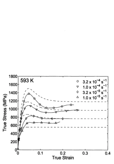
![Figure 3-5: Stress-strain curves from Vitreloy-1 from Lu et al. [2]. The solid are results from the model.](https://thumb-eu.123doks.com/thumbv2/123doknet/14459396.520205/60.918.260.645.292.923/figure-stress-strain-curves-vitreloy-solid-results-model.webp)