HAL Id: hal-00940961
https://hal-enac.archives-ouvertes.fr/hal-00940961
Submitted on 18 Mar 2014
HAL is a multi-disciplinary open access archive for the deposit and dissemination of sci-entific research documents, whether they are pub-lished or not. The documents may come from teaching and research institutions in France or abroad, or from public or private research centers.
L’archive ouverte pluridisciplinaire HAL, est destinée au dépôt et à la diffusion de documents scientifiques de niveau recherche, publiés ou non, émanant des établissements d’enseignement et de recherche français ou étrangers, des laboratoires publics ou privés.
Ground-based prediction of aircraft climb : point-mass
model vs regression methods
Richard Alligier, Mohammad Ghasemi Hamed, David Gianazza, Mathieu
Serrurier
To cite this version:
Richard Alligier, Mohammad Ghasemi Hamed, David Gianazza, Mathieu Serrurier. Ground-based prediction of aircraft climb : point-mass model vs regression methods. Complex World 2011, 1st Annual Complex World Conference, Jul 2011, Seville, Spain. pp xxxx. �hal-00940961�
Ground-based prediction of aircraft climb:
point-mass model vs. regression methods
R. Alligier, M. Ghasemi Hamed, D. Gianazza
DSNA Toulouse, France
M. Serrurier
Institut de Recherche en Informatique de Toulouse, France
INTRODUCTION
Predicting aircraft trajectories with great accuracy is central to most operational concepts ([1], [2]) and automated tools that are expected to improve the air traffic management (ATM) in the near future.
On-board flight management systems predict the air-craft trajectory using a point-mass model describing the forces applied to the center of gravity. This model is formulated as a set of differential algebraic equations that must be integrated over a time interval in order to predict the successive aircraft positions in this interval. The point-mass model requires knowledge of the aircraft state (mass, thrust, etc), atmospheric conditions (wind, temperature), and aircraft intent (target speed or climb rate, for example).
Many of these informations are not available to ground-based systems, and those that are available are not known with great accuracy. The actual aircraft mass is currently not transmitted to the ATM ground sys-tems, although this is being discussed in the EUROCAE group in charge of elaborating the next standards for air-ground datalinks. The atmospheric conditions are estimated through meteorological models. Finally, the current ground-based trajectory predictors make fairly basic assumptions on the aircraft intent (see the "airlines procedures" that go with the BADA1 model). These
default "airline procedures" may not reflect the reality, where the target speeds are chosen by the pilots ac-cording to a cost index that is a ratio between the cost of operation and the fuel cost. These costs are specific to each airline operator, and not available in the public domain.
As a consequence, ground-based trajectory prediction is currently fairly inaccurate, compared to the on-board prediction. A simple solution would be to downlink the on-board prediction to the ground systems. However, this
1BADA: Base of Aircraft Data
is not sufficient for all applications: some algorithms (citation AlliotDurand) require the computation of a mul-titude of alternate trajectories that could not be computed and downlinked fast enough by the on-board predictor. There is a need to compute trajectory predictions in ground systems, for all traffic in a given airspace, with enough speed and accuracy to allow a safe and efficient 4D-trajectory conflict detection and resolution.
In this paper, we compare different ways to address this trajectory prediction problem, focusing on the air-craft climb with a 10 minutes look-ahead time. As a first approach, the point-mass model is tried with different settings for the model parameters, considering a con-stant CAS/Mach climb procedure where the aircraft first climbs at a constant Calibrated Air Speed (CAS) until it reaches the CAS/Mach crossover altitude and continues the climb at a constant Mach number. In this approach, the basic parameter setting consists in using the standard CAS and Mach values of the BADA climb procedures file, and a standard reduced thrust during climb, with an average reference aircraft mass. The second setting still uses the reference mass and standard thrust reduction factor, but the actual CAS is computed from the past aircraft positions.
The second approach is radically different and is based on regression methods. The predicted aircraft position is considered as a function f(x, θ) where x is a vector of of input variables and θ a vector of parameters. In our case, the input variables are the past aircraft positions, the observed CAS at the current altitude, the deviation of the air temperature from the standard atmosphere, and the predicted wind at different flight levels. The parameters (vector θ) must be adjusted using historical data so that the computed output fits the observed position as best as possible. Three regression methods are tried. In the first one, the function f is an artifial neural network predicting a couple (d, z) (along-track distance, altitude). In the second method, genetic programming is
used to find a function f predicting the altitude z: an initial population of functions follows a darwinian-like evolution during several generations, with crossovers, mutations, and selection of the best predictors at each generation. The third method uses fuzzy regression to predict a possibility function describing the uncertainties on the future aircraft position, instead of a single position or altitude as in the two other regression methods.
The rest of this paper is organized as follows: ...
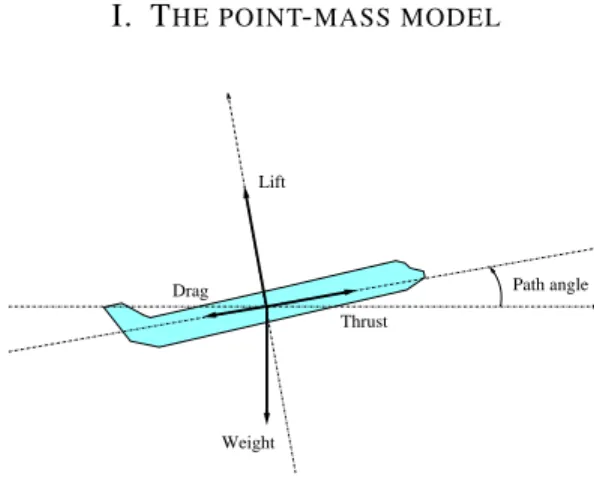
I. THE POINT-MASS MODEL
Path angle
Weight Lift
Thrust Drag
Figure 1. Simplified point-mass model.
A. Simplified equations
Most ground systems use a simplified point-mass model, sometimes called total energy model, to predict aircraft trajectories. This model, illustrated on figure 1, describes the forces applying to the center of gravity of the aircraft and their influence the aircraft acceleration, making several simplifying assumptions2. It is assumed
that the thrust and drag vectors are colinear to the airspeed vector, and that the lift is perpendicular to these vectors. Thus, projecting the forces on the airspeed vector axis, the longitudinal acceleration a = dVTAS
dt along
the true airspeed (VTAS) axis can be expressed as follows:
m.a = T − D − m.g.sin(γ) (1)
where T is the total thrust, D the aerodynamic drag of the airframe, m the aircraft mass, g the gravitational acceleration, and γ the path angle (i.e. the angle between the airspeed vector and the horizontal plane tangent to the earth surface).
2Note that more complex point-mass models have been proposed
for UAV or fighter airplanes (see [3]), modeling also the side-slip angle.
Introducing the rate of climb/descent dh dt =
VTAS.sin(γ), where h is the altitude in meter, this
equa-tion can be rewritten as follows (see [4]):
(T − D).VTAS = m.VTAS.
dVTAS
dt + m.g. dh
dt (2)
Sereral equivalent forms of this equation can be used (see Eurocontrol BADA3 User Manual), depending on
what unknown variable is being calculated from the other known variables.
Actually using equation 2 to predict a trajectory re-quires a model of the aerodynamic drag for any airframe flying at a given speed through the air. In addition, we may need the maximum thrust, which depends on what engines the aircraft is equipped with. In the experiments presented here, the Eurocontrol BADA model was used to that purpose.
In addition, one cannot use equation 2 without prior knowledge of the initial state (mass, position, speed,...) of the aircraft, and also of the pilot’s intents as to how the aircraft will be operated in the future (thrust law, speed law, or rate of climb). When the aircraft is operated at a given calibrated air speed (CAS4) or mach number,
computing the true air speed (TAS) requires knowledge of the atmospheric conditions (the air temperature and pressure). Finally, as we need to predict the trajectory over the ground surface, and not only through the air, the wind intensity and direction are also required.
B. Aircraft operation during climb
Generally, when no external constraints apply during the climb, the aircraft is operated at constant CAS5 and
variable Mach number, until a specified Mach number is reached. Above this CAS/Mach crossover altitude, the aircraft is operated at a constant Mach number, and variable CAS. External constraints may apply, however. After take-off, the aicraft cannot exceed a specified maximum CAS until Flight Level 1006 is reached. This
first climb segment is followed by an acceleration at FL100, and then a second climb segment at a higher calibrated air-speed, until the CAS/Mach crossover alti-tude is reached.
In this paper, we shall consider only this second climb segment at constant CAS, followed by the constant Mach climb, as we are mostly interested in predicting the
3BADA: Base of Aircraft DAta
4CAS: Calibrated Air Speed, which can be assimilated to the speed
indicated on the pilot’s intruments.
5CAS: Calibrated Air Speed.
aircraft trajectory in the en-route airspace. Note that some other air traffic control constraints may apply, that modify the aircraft operation during climb. For instance, the aircraft may be operated at a chosen rate of climb, on some flight segments, in order to be above a specified flight level over a given waypoint.
Even without such constraints, and assuming a climb at constant CAS/Mach, predicting the aircraft trajectory is not easy for ground systems. The actual CAS and Mach values are chosen by the airlines’ operators, ac-cording to a cost index specific to each airline. The cost index, and the chosen CAS and Mach values, are not known to air traffic control systems today, although some studies show the improvements that such knowledge would provide in the trajectory prediction ([5], [6]).
II. REGRESSION METHODS
Regression methods aim at predicting an output y as a function of a given input x and a vector of parameters θ:
y = f (x, θ) (3)
In our trajectory prediction problem, we shall predict one of the following outputs, depending on the chosen method:
• a couple (d(t), z(t)) where d is the horizontal
distance flown by the aircraft and z its altitude at time t > t0, where t0 is the current time,
• only the altitude z(t),
• or possibility distributions Πd(t) and Πz(t)
char-acterizing the uncertainties on the values of d and z at time t. These possibility distribu-tions can be approximated by two quadruples Πd(t) = (d1(t), d2(t), d3(t), d4(t)) and Πz(t) =
(z1(t), z2(t), z3(t), z4(t)) as illustrated on figure (*
FIGURE TBD *).
The input x shall be a vector of values extracted from the following values:
• the current and previous aircraft states,
character-ized by z[k], d[k], CAS[k], Mach[k], with k ∈ [−10, 0]. The past trajectory is sampled every δt seconds. z[k] denotes the value measured for the altitude z at time t = t0+ k.δt. With this notation,
z[0] = z(t0) is the current altitude, z[−1] is the
altitude δt seconds before t0, and so on. The same
notation applies for d, CAS and Mach,
• the difference between the actual air temperature at
sea level and the air temperature of the International Standard Atmosphere (ISA) at sea level,
• the along-track and cross-track wind w and the
temperature T at different altitudes.
The parameters θ must be adjusted using historical data, so that the computed outputs are as close as possible to the observed data. The performance of the tuned model shall be measured by assessing how the model generalizes on fresh inputs. k-fold cross validation can be used for that purpose.
In order to start with a relatively simple problem, we shall predict only one point (or one couple of fuzzy sets) of the future trajectory, N steps ahead. Let us now shortly describe the regression methods that are used to predict this future aircraft position (or uncertainty intervals).
III. REGRESSION USING NEURAL NETWORKS(NN)
Artificial neural networks are algorithms inspired from the biological neurons and synaptic links. An artificial neural network is a graph, with vertices (neurons, or units) and edges (connections) between vertices. There are many types of such networks, associated to a wide range of applications. Beyond the similarities with the biological model, an artificial neural network may be viewed as a statistical processor, making probabilistic assumptions about data ([7]). The reader can refer to [8] and [9] for an extensive presentation of neural networks for pattern recognition.
In our experiments, We used a specific class of neu-ral networks, referred to as feed-forward networks, or multi-layer perceptrons (MLP). In such networks, the units (neurons) are arranged in layers, so that all units in successive layers are fully connected. Multi-layers perceptrons have one input layer, one or several hidden layers, and an output layer.
For a network with one hidden layer, the output vector y = (y1, ..., yk, ..., yq)T is expressed as a function of the
input vector x = (x1, ..., xi, ..., xp)T as follows:
yk= Ψ( q X j=1 θjkΦ( p X i=1 θijxi+ θ0j) + θ0k) (4)
where the θij and θjk are weights assigned to the
connections between the input layer and the hidden layer, and between the hidden layer and the output layer, respectively, and where θ0j and θ0k are biases
(or threshold values in the activation of a unit). Φ is an activation function, applied to the weighted output of the preceding layer (in that case, the input layer), and Ψ is a function applied, by each output unit, to the weighted sum of the activations of the hidden layer. This
expression can be generalized to networks with several hidden layers.
The output error – i.e. the difference between the desired output (target values) and the output y computed by the network – will depend on the parameters θ (weights and biases), that must be tuned by training the network, so as to minimize a chosen function of the output error. In our case, the minimized function is the sum of quadratic errors. The optimization method is either a gradient descent with momentum, or a BFGS quasi-Newton method. The activation function is the logistic sigmoôrd, and the output function is the identity. Neural network have already been applied to trajectory prediction, in [10]. However, they were used to predict both the climb and cruise flight segments, given a requested flight level, and lateral navigation as well. This approach, where the altitude error is likely to be small after the cruise flight level has been captured, is difficult to compare to our approach focused on minimizing the prediction error on the climb segment only. A mix of neural networks proved efficient for the chosen purpose, though.
IV. REGRESSION USINGGENETICPROGRAMMING
(GP)
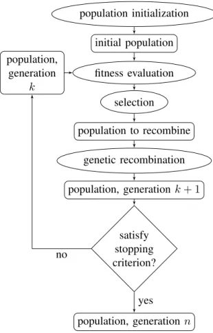
Genetic Programming (GP) is part of the Evolution Algorithm family. It is a population-based algorithm as can be seen on figure 2. Each individuals of the population encodes a computer program. A fitness crite-rion is assigned to those computer programs according their capacity in doing a predifined task. These fitnesses are then used for selecting individuals to recombined, giving then a new population. This approach is inspired from biology principles like genetic recombination and Darwinian selection principle.
In GP as it was popularized in [11], individuals are represented by a tree. They have a variable length. Typically, leafs contain inputs from the terminal set T , and nodes contain functions from the function set F which will be applied to the evaluation of its children. [11] has also defined a standard crossover and a standard mutation operation.
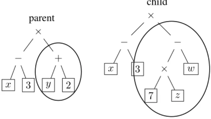
In a standard crossover, one subtree is randomly se-lected on each parents, and then the two sese-lected subtree are then exchanged, as illustrated in figure 3.
In a standard mutation, one subtree is randomly se-lected and is then replaced by a generated tree, as showed in figure 4.
These recombination operators implies the closure property. Each functions shall accept any elements in
population initialization initial population fitness evaluation selection population to recombine population, generation k genetic recombination population, generation k + 1 satisfy stopping criterion? population, generation n no yes
Figure 2. Flow chart of Evolutionary Algorithms.
parent P1 × − x 1 × y 2 parent P2 + + x y + 5 2 child C1 × + 5 2 × y 2 child C2 + + x y − x 1
parent × − x 3 + y 2 child × − x 3 − × 7 z w
Figure 4. Standard mutation.
T and any output of the functions in F .
1) Our terminal set T and function set F : We have to find a function f(x, θ) parametrized by θ which predicts a variable y from a vector of input variables x = (x1, . . . , xn). A natural way to do that is to take
T = {x1, . . . , xn, ℜ} and F = {+, ∗, −, /, cos, sin}
for instance, with ℜ a variable which is replaced by a randomly generated constant at the creation of the tree. In fact, this method to generate constant terms in our expression is said to be inefficient. In order to cope with this issue, we have hybridized GP with a multiple regression technique, the Ridge regression [12]. The execution of a tree gives us a set of func-tions G = {g1, . . . , gk} which will be used to build
a function f(x, {λ0, . . . , λk}) = λ0 + k
P
i=1
λigi(x) with
its parameters adjusted by a Ridge regression. The gi
generated are piecewise monomials. We have defined T = {{x1} , . . . , {xp}}. If we consider n input variables
x1, . . . , xn, N instances in our training set and two sets
A = {a1, . . . , akA} and B = {b1, . . . , bkB}, we have
build operators to combine these two sets of functions A and B: • ⊕(A, B) = A ∪ B • ⊗(A, B) = kA ∪ i=1{ai.b1, . . . , ai.bkB} • ∆i,p(A, B) = {δ({xi ≤ vi,p} , a1), . . . , δ({xi ≤ vi,p} , akA)} ∪ {δ({xi > vi,p} , b1), . . . , δ({xi> vi,p} , bkB)} with :
– vi,p, the p-th bigger value of xiobserved in our
training set.
– δ(CON D, expr)(x) = (
expr(x) if ∀ cond ∈ COND, cond(x)
0 otherwise
where x is an instance.
With these definitions, we can notice that:
• δ(CON D1, expr1).δ(CON D2, expr2) =
δ(CON D1∪ CON D2, expr1.expr2) • δ(CON D1, δ(CON D2, expr2)) =
δ(CON D1∪ CON D2, expr2)
• CON D defines a multi-dimensionnal interval
though it can be simplified. For instance {8 < x1, 9 < x1, x1≤ 14, x1 ≤ 15} can be
simplified in {9 < x1, x1 ≤ 14}. Thus, no more
than two conditions have to be associated with one variable xi, making conditions sets easy to
compare between each other.
In our implementation we have chosen F =
{⊕, ⊗}S n ∪
i=1 N −1
∪
p=1 {∆i,p} as the function set.
Con-sequently, we can assume that the set encoded by a tree only contains expressions such as Qn
i=1 xki i or δ(CON D, n Q i=1 xki
i ) with ki ∈ N. Thus, expressions are
easy to compare, making the ∪ operation manageable on our function sets.
With this choice, f(x, {λ0, . . . , λk}) is a piecewise
polynomial. Conditions are used there as we assume that the trajectory prediction problem to be piecewise.
2) Fitness criterion: We have to assess a fitness to each candidate function f(x, {λ0, . . . , λk}). We want
this function to make good prediction on unseen data. Typically, we learn parameters λ0, . . . , λk from a finite
training set containing N instances. Using those N instances, the more we have parameters, the less their es-timation will be reliable. In order to take into account this issue, we have used the AICc criterion [13], [14] defined
as AICc = N.log(M SE) + 2(k + 2) +2(k+2)(k+3)N −k−2 with
M SE = min λ0,...,λk∈R 1 N N P i=1 (y(i)− f (x(i), {λ 0, . . . , λk}))2.
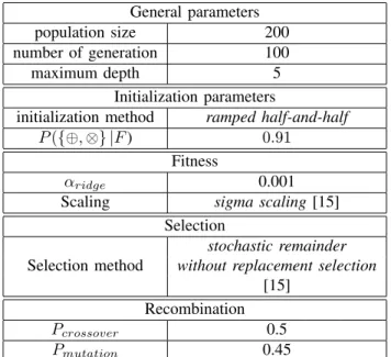
The algorithm was parametrized as follow :
T = ROCD + CAS + DCAS +
M ACH + DM ACH + ESF + Dtemp0ISA +
WalongFL190 + WcrossFL190 + T empFL190 +
WalongFL250 + WcrossFL250 + T empFL250 +
WalongFL310 + WcrossFL310 + T empFL310 +
WalongFL340 + WcrossFL340 + T empFL340 +
WalongFL370 + WcrossFL370 + T empFL370 +
DdAIRminus9 + DdAIRminus7 + Dzminus7 +
DdAIRminus5 + Dzminus5 + DdAIRminus3 +
General parameters
population size 200
number of generation 100
maximum depth 5
Initialization parameters
initialization method ramped half-and-half
P ({⊕, ⊗} |F ) 0.91
Fitness
αridge 0.001
Scaling sigma scaling[15]
Selection
stochastic remainder
Selection method without replacement selection
[15] Recombination
Pcrossover 0.5
Pmutation 0.45
V. INTERVAL REGRESSION USINGKNEAREST NEIGHBOURS(I-KNN)
A. Possibility theory
Possibility theory, introduced Zadeh [16], [17], was initially created in order to deal with imprecision and uncertainty due to incomplete information. This kind of uncertainty may not be handled by probability theory, especially when a priori knowledge about the nature of the probability distribution is lacking. A possibility distribution π is a function from Ω, the universe of dis-course (R in our case), to (R → [0, 1]). The definition of the possibility measure Π is based on the the possibility distribution π such that :
Π(A) = sup(π(x), ∀x ∈ A). (5)
The α-cut of a possibility distribution Aα is the interval
for which all the points located inside, have a possibility membership π(x) greater or equal to α. We have :
Aα= {x|π(x) ≥ α, x ∈ Ω}. (6)
One interpretation of possibility theory is to consider a possibility distribution as a family of probability dis-tributions (see [18] for an overview). Thus, a possibility distribution π will represent the family of the probability distributions Θ for which the measure of each subset of Ω will be bounded its possibility measures :
Θ = {P |∀A ∈ Ω, P (A) ≤ Π(A)}. (7) Given a probability distribution p, a confidence interval Iα is a subset of Ω such as P (Iα) = α. We define
I∗
α, also referred as quantile, as the smallest confidence
Figure 5. The maximum specified possibility distribution for N(0,1).
interval with probability measure equal to α. Thus, an alternative of the equation 7 is:
∀α ∈ [0, 1], p ∈ Θ, I∗
p,(1−α) ⊆ Aα. (8)
Thus, a possibility distribution encode a family of distri-butions for which each quantile is bounded by α-cuts. In many cases it is desirable to move from the probability framework to the possibility framework. Probability-possibility transformation [19] is based on the maximum specificity principle. Given a probability distribution p, what we obtain is the possibility distribution π∗ which is
the most specific one that bound p. Given p we compute π∗ as follows :
∀x ∈ Ω, pi∗
(x) = maxα,x∈Iα(1 − α). (9)
Then, in the spirit of equation 8, given p and its trans-formation π∗ we have :
A∗
1−α = Iα∗
Figure 5 presents the maximal specific transformation of a normal distribution p is the π possibility distribution.
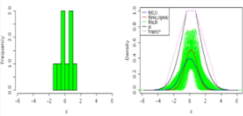
B. Possibility distribution for a Gaussian family com-puted on a set of data
When we suppose that our data comes from a Normal distribution with unknown mean (µ) and variance (σ2).
The solution that comes immediately to our mind is to estimate µ and σ from the data. However, computing a value of these parameters that is statistically faithful requires a lot of data. One solution is to compute confidence intervals confidence interval for the mean and the variance. Based of the χ2 distribution, the confidence
intervals [µmin, µmax] and [σmin, σmax] will contains
respectively 95% of the possible values for µ and σ given a set of data. We propose to compute the maximal specific possibility distribution that contains all the nor-mal distributions that have parameters in the confidence intervals (Θ = {g|g = N(µ, σ2), µ ∈ [µ
min, µmax], σ2 ∈
[σ2
min, σmax2 ]}). We compute le possibility distribution
π∗
Θ as follows :
Figure 6. An example of the possibility distribution for the family Θ, with a confidence level of 0.95 and a dataset with n=10.
• ∀x < µmin : πΘ∗(x) = sup(1 − P (Iα∗), x ∈ Iα∗) with
p = N (µmin, σmax2 )
• ∀x > µmin : πΘ∗(x) = sup(1 − P (Iα∗), x ∈ Iα∗) with
p = N (µmax, σ2max)
where G is the probability measure associated with the density g. In the following, in a simplification purpose, we will call respectively, the normal distribution built from the estimated mean and the estimated variance and the maximum specified possibility distribution encoding the family Θ described above, N(µe, σe) and π∗Θ. Figure
6 present the distribution π∗
Θ for a data set of size 10
that follows a Gaussian distribution. In this figure the Θ family is represented by a set of green distribution functions N(a, b), the distribution π∗
Θ is in black. When
the dataset size grows, π∗
Θ converges to the normal
distribution.Thus, the size of π∗
Θ(his specificity) depends
on the quantity of data available and allows us to have a statistically significant representation of the data.
C. K-nearest neighbours (KNN)
The k-nearest neighbours(KNN) algorithm is a re-gression method which finds the response value of the input data based on closest training instances. For any given input instance X, the KNN algorithm finds the K nearest instances (KsetX) and chooses the mean of their
response values (Y ) as the estimated value (Yestimated).
In our case, we are not only interested in obtaining the most probable position of the plane, but we are also interested to find the interval which contains the response value with an high probability. With global regression approaches, this interval can be computed by using the standard deviation of the error (RMSE). Since it is a global estimation, the size of the interval is constant, so it does not depend on the inputs. Moreover, it supposes that the distribution of the error follows an a priori known distribution (usually a Gaussian one) and that we have enough data to estimate precisely the parameters. The advantage of the KNN algorithm is that it can give a
local estimation of the data distribution. However, the imprecision about the parameters of the function depends on the value of k. When k is high the parameters are precise, but the distribution will contain a lot of data that are different to the input one. Then, quantile will be very large. On the contrary, if k is low, the k-set will contain data that are close to the input but the imprecision about the parameters of the distribution will be high. In our method, we propose, given k, to compute the possibility distribution that bounds all the Gaussian distributions that may have generated the k-set (see previous section). For each input value we choose the value of k that is the best trade off between the precision and the size of the quantile. The algorithm is described in Alg The idea
Algorithm 1 For any input X, finds the minimum interval which should contain the response value
1: KsetX ← Find the K nearest neighbours of X
2: M INK ← K
3: IntervalSizemin← Inf
4: for all i ∈ 5, . . . , K do
5: Compute [µmin, µmax] and [σmin, σmax] w.r.t. the
i-th first example in KsetX
6: IntervalSize ← G−1(0.975, µ
max, σmax2 ) −
(G−1(0.25, µ
min, σ2max)
7: if IntervalSize ≤ P IIntervalSizemin then
8: M INK ← i
9: IntervalSizemin ← IntervalSize
10: end if
11: end for
of the approach is to have intervals that guarantee to contain the expect quality of data. For instance, given k, the 0.05-cut of π∗
Θ will contain at least 95% of
the data since it contains the 0.95 quantiles of all the Gaussian distribution that may have generated the k-set. This approach may be useful for instance for detecting conflict or for defining safe area zone because it will take into account all the cases that are statistically possible.
VI. DATA AND EXPERIMENTAL SETUP
A. Data pre-processing
Recorded radar tracks from Paris Air Traffic Control Center were used to build the patterns used in the re-gression methods. This raw data is made of one position report every 1 to 3 seconds, over two months (july 2006, and january 2007). In addition, the wind and temperature data from Meteo France are available at various isobar altitudes over the same two months.
The raw Mode C altitude7 has a granularity of 100
feet. So the recorded aircraft trajectories were smoothed, using a local quadratic model, in order to obtain: the aircraft position (X,Y in a projection plan, or latitude and longitude in WGS84), the ground velocity vector (Vx, Vy), the smoothed altitude (z, in feet above isobar
1013.25 hPa), the rate of climb or descent (ROCD). The wind (Wx, Wy) and temperature (T ) at every trajectory
point were interpolated from the meteo datagrid. The temperature at isobar 1000 hPa was also extracted for each point, in order to compute a close approximation of (∆T0)ISA, the difference between the actual temperature
and the ISA model temperature at isobar 1013.25 hPa (mean sea level in the ISA atmospheric model). This (∆T0)ISA is one of the key parameters in the BADA
model equations.
Using the position, velocity and wind data, we com-puted the true air speed (TAS), the distance flown in the air (dAIR), the drift angle, the along-track and cross-track winds (Walong and Wcross). The successive velocity vectors allowed us to compute the trajectory curvature at each point. The actual aircraft bank angle was then derived from true airspeed and the curvature of the air trajectory. The climb, cruise, and descent segments were identified, using triggers on the rate of climb or descent to detect the transitions between two segments.
Finally, the BADA model equations were used to compute additional data, such as: calibrated airspeed (CAS), Mach number (M), energy share factor8 (ESF),
as well as the derivatives of these quantities with respect to time.
B. Filtering and sampling climb segments
As our aim is to compare several prediction models, we focused on a single aircraft type (Airbus A320), and selected all flights of this type departing from Paris Orly (LFPO) or Paris Roissy-Charles de Gaulle (LFPG). The trajectories were then filtered so as to keep only the climb segments. An additionnal 40 seconds were clipped from the beginning and end of each segment, so as to remove climb/cruise or cruise/climb transitions.
The trajectories were then sampled every 15 seconds, with time and distance origins at the point P0 where the
climb segment crosses flight level FL1809. The trajectory
7This altitude is directly derived from the air pressure measured
by the aircraft. It is the height in feet above isobar 1013.25 hPa.
8The energy share factor (ESF) says how much of the energy is
devoted to climb or to longitudinal acceleration.
9FL180: 18000 feet above isobar 1013 hPa.
segments were sampled so as to obtain 10 points preced-ing P0, and a number of points after P0, depending on
the chosen look-ahead time. So the trajectory observed during the preceding time steps (2 minutes 30 seconds), can be used to predict the aircraft position at one or several future time steps. The predicted position can be compared to the actual aircraft position at the same time step.
Trajectories exhibiting a bank angle greater than 5 degrees were discarded, so that the influence of trajectory turns on the rate of climb can be neglected. This allows us to disregard the lateral navigation in our trajectory prediction problem, and focus on the longitudinal and vertical dimensions of the trajectory.
C. Building patterns for regression
The regression models y = f(x, θ) are tuned and assessed using sets of patterns (x, d), where x is an input vector, and d is the corresponding desired output that can be compared to the computed output y. These patterns, that we have already described in section II were extracted from the sampled climb segments. 1500 patterns were randomly chosen, to build the set used in our experiments.
Each pattern used for regression contains the current ground speed, true and calibrated air speed, Mach num-ber, and their derivatives with respect to time, the energy share factor, the altitude variations and distance flown for the ten preceding time steps, and also the predicted wind and temperature at several altitudes that the aircraft may cross in the look-ahead time. It also contains the target variables: distance flown, in the air or above the ground, and altitude reached after N time steps in the future. D. Principal component analysis
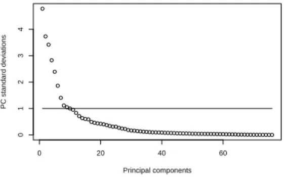
The final patterns set contains 79 numerical variables, measured for 1500 aircraft climbs. There are 76 explana-tory variables, and 3 variables to explain. A principal component analysis was performed on the explanatory variables, so as to reduce the dimensonality and avoid redundant input variables in the trajectory prediction.
Figure 7 shows the standard deviations of the principal components: 9 components have a standard deviation above 1, and 7 other components are between 0.5 and 1. Principal components are linear combinations of the initial variables, that we can use as explanatory variables in the regression method. This reduces the dimensonality to 10 to 15 significant principal components, instead of the 76 initial variables. One must keep aware, however, that using linear combinations representing projections
0 20 40 60 0 1 2 3 4 Principal components PC standard de viations
Figure 7. Principal components standard deviations.
on a basis of orthogonal vectors may not take account of some non-linearities in the initial variables.
E. Experimental setup
The methods applied to our prediction problem for climbing aircraft are listed in table I.
BADA BADA point-mass model, using the reference mass for each aircraft and BADA values for the constant CAS/Mach, assuming reduced climb (eq. 3.8.1 and 3.8.2, p.22 in [4]), and taking account of the (∆T0)ISA temperature
differ-ence.
BADA(obs) Same BADA model as above, but using the CAS observed at t0, and the BADA target
Mach number
LR Ordinary least squares linear regression NN Regression with neural networks
GP Regression with genetic programming, using Akaike’s AIC to assess the fitness of each prediction function in the population. I-KNN Interval regression using K-nearest neighbours,
returning intervals of uncertainty Table I
METHODS APPLIED TO ALTITUDE PREDICTION
In our experiments, these methods are scored using a 10-fold cross-validation on the dataset described in section VI-C. This set is split in ten subsets. Nine of these subsets are used to tune the model parameters θ, and the remaining subset is used to assess the model performance. This operation is repeated 10 times, cycling through the subsets. The models’ performace is assessed over the ten runs, considering the mean score, the standard deviation, and also confidence intervals for the computed output.
Uncertainty on the prediction can be assessed in sev-eral ways. Once the model parameters have been tuned on the training set (i.e. the concatenation of 9 subsets
used in cross-validation), we can compute a theoritical 95%-confidence interval using the root mean square error (RMSE) observed on this training set, assuming a Gaussian distribution of the error in altitude (and also in distance, if predicted). We can then count how many instances of the validation subset actually fall within this confidence interval.
We can also assess the uncertainty on the predicted altitude (or distance) by considering the actual distribu-tion of errors in the training set. We can then assume a Gaussian distribution, but with some uncertainty on the mean value and standard deviation. This gives us a family of Gaussian distributions from which we can compute a possibility distribution (see section V-B). This is the approach chosen in the possibilistic regression using K-nearest neighbours. For every instance in the validation set, the K nearest instances of the "training set"10 are found, using a distance between vectors of
variables. The possibility distribution is computed on these K neighbours. In theory, the 0.05-cut of this possibility distribution is guaranteed to contain at least 95% of the data. We can then check if our instance in the validation set falls within this interval or not. This is repeated for all instances in the validation set, such providing the ratio of predictions actually within the confidence interval of variable size (there is an interval for each instance).
VII. RESULTS Method MAE RMSE BADA 1440 (79) 1824 (95) BADA(obs) 1440 (77) 1819 (86) LR 745 (35) 965 (47) NN 841 (47) 1080 (55) GP 744 (28) 964 (41) I-KNN - -Table II
AVERAGE PREDICTION ERRORS(AND STANDARD DEVIATIONS)
ON THE ALTITUDE(IN FEET)FORAIRBUSA320AIRCRAFT,USING
15PRINCIPAL COMPONENTS AS INPUT,WITH THE REFERENCE
POINT ATFL180AND A10-MINUTES LOOK-AHEAD TIME.
Table II shows the prediction errors (mean absolute error, and root mean squared error) over the 10 runs of the cross-validation, for all tested methods. The 15 prin-cipal components of higher variance were used as input to the regression methods. This selection was made by
10This is not actually a training set, as there is no training when
prior trials, adding successively the principal components until no significant improvement was observed.
All regression methods perform significantly better than the BADA point-mass model. There are several factors explaining the poor performance of the point-mass models. The parameters’choice assumed a constant CAS/Mach climb at economic thrust, and the same reference mass for all aircraft, which is actually not the case in reality. Also, the regression method use the past trajectory to predict the future altitude, whereas our BADA models do not. Using the observed CAS instead of the BADA standard CAS does not improve the results on altitude prediction.
We also observed that the mean predicted altitude with BADA models is biased toward lower altitudes. The mean error, averaged over the 10 runs, is −735 feet for the first BADA model, and −603 feet for the second BADA model. After some investigation, it appears that the CAS is highly sensitive to the air density, and that much more realistic values are obtained when using a more accurate temperature model (Meteo France data at successive altitudes) than when extrapolating from (∆T0)ISA. At the time of this publication, this was not
implemented in our BADA model. It is expected that it would give errors more centered around zero, but with a similar dispersion than today’s implementation.
It came as a surprise that non-linear regression meth-ods did not perform better than the ordinary least squares linear regression. There may be several explanations to this. Using the principal components as inputs does favour linear methods. In addition, tuning the parameters with the ordinary least squares linear regression can be done with an exact method, whereas non-linear methods require iterative approximations, that may have difficul-ties to find the optimum when using very noisy data.
Method Ratio in the-oretical 95% interval Theoretical 95% |δz| Actual 95% |δz| BADA 0.92 (0.025) 3279 (20) 3593 (249) BADA(obs) 0.93 (0.021) 3369 (19) 3674 (260) LR 0.94 (0.013) 1863 (10) 2015 (187) NN 0.905 (0.030) 1846 (92) 2203 (215) GP 0.93 (0.019) 1818 (26) 1923 (162) I-KNN 0.986 3376 (714) -min. 417 max. 6082 Table III
UNCERTAINTY ON THE ALTITUDE PREDICTION(AIRBUSA320),
FOR A REFERENCE POINT ATFL180AND A10-MINUTES
LOOK-AHEAD TIME.
Some results on the uncertainty of the altitude predic-tion are shown in Table III. The second column shows the ratio of predictions, computed with instances from the validation set, that actually fall within the 95% confidence interval computed using the training set. For all methods but I-KNN, this interval is simply the in-terquantile interval corresponding to the 95% confidence, assuming a Gaussian distribution of the error. For I-KNN, this is the 0.05-cut of the possibility distribution computed from a family of Gaussian distributions. The third column shows the width of this theoretical interval. As this interval is of variable size for I-KNN, the lower, mean, and higher half-width observed on all instances are given. The last column shows the actual value of |δz|
(the interval half-width) for which 95% of the observed altitudes zobs fall in the interval [z − δz, z + δz], where
z is the predicted altitude.
CONCLUSION
In this paper, we have applied several methods to the prediction of altitude, focusing on a single aircraft type (A320). The aim was to compare these methods when predicting the altitude of climbing aircraft 10 minutes ahead, starting from an initial point at flight level FL180, and possibly using the past trajectory to improve the prediction. Radar and Meteo data recorded over two months (july 2006, january 2007) were used to build a dataset of explanatory and target variables. A principal component analysis of this data allowed us to reduce the dimensionality to 10 to 15 significant components, in-stead of the 76 initial explanatory variables. The models are compared by performing a 10-fold cross-validation on a set of 1500 climb segments.
Our results show that the regression methods perform better than the point-mass model. This is not surprising as the former learn from the observation of the past trajectory, whereas the point-mass model uses the same standard values for most parameters (mass, power reduc-tion, target speeds) for all aircraft. The genetic program-ming approach proved efficient, although not better, on our noisy data, than standard regression methods.
Two different kinds of predictive methods have been applied to our problem, with two different ways to compute confidence intervals on the predicted altitude. In the first approach (LR, GP, NN, and also BADA models), the target variable to predict is the altitude itself. A probabilistic confidence interval can be obtained by considering the interquantile interval, assuming a Gaussian distribution of the error. This confidence inter-val, although statistically relevant when measured on an
infinity of instances, is not guaranteed to actually contain the expected ratio of accurate predictions (e.g. 95%) for a limited number of instances. This explains why we observed less than 95% of the predictions actually falling in the theoretical confidence interval, with these methods.
In the second approach, the interval regression using K-nearest neighbours (I-KNN) returns a confidence in-terval, instead of the altitude itself. This method still assumes a Gaussian distribution of the error, but with some uncertainty on the distribution’s parameters. This gives a family of probability distributions, from which we can deduce a possibility distribution. I-KNN com-pute one such possibility distribution for each instance, using the instance’s nearest neighbours in the examples’ dataset. So the size of the confidence interval obtained from this distribution depends on the quantity of data in the neighborhood of the considered instance. Obviously, these intervals are generally larger than the probabilistic confidence intervals obtained with standard methods. However, they are statistically guaranteed to contain at least the expected ratio of accurate predictions. This is confirmed in our experiments, where we found 98.6% instances actually falling in the 95% confidence interval. From an operational point of view, the proposed methods could be applied to the detection of poten-tial conflicts between trajectories. Standard regression methods could be used to provide a relatively narrow probabilistic interval allowing us to detect conflicts with a great look-ahead time, although with some uncertainty. With smaller look-ahead times, when more certainty is required before actually deviating conflicting trajectories, interval regression could provide guaranteed confidence intervals on the altitude prediction.
In future works, we plan to conduct a more thorough analysis of the available data, trying to filter the climb segments according to the actual aircraft mode of oper-ation (constant CAS or constant ROCD, for example), so as to obtain less noisy data. We could then learn the aircraft climbs in a specific operation mode, thus giving a better chance to the point-mass model. It could also be interesting to learn some of the point-mass model parameters (mass, thrust law) from the observed data. Concerning the regression methods, we could try to im-prove the genetic programming approach by introducing elements of the point-mass model in the population of predictors.
REFERENCES
[1] SESAR Consortium. Milestone Deliverable D3: The ATM
Target Concept. Technical report, 2007.
[2] H. Swenson, R. Barhydt, and M. Landis. Next Generation Air Transportation System (NGATS) Air Traffic Management (ATM)-Airspace Project. Technical report, National Aeronau-tics and Space Administration, 2006.
[3] F. Imado T. Kinoshita. The application of an uav flight simulator - the development of a new point mass model for an aircraft. In SICE-ICASE International Joint Conference Conference, 2006. [4] A. Nuic. User manual for base of aircarft data (bada) rev.3.7.
Technical report, EUROCONTROL, 2009.
[5] R. A. Coppenbarger. Climb trajectory prediction enhancement using airline flight-planning information. In AIAA Guidance, Navigation, and Control Conference, 1999.
[6] Study of the acquisition of data from aircraft operators to aid trajectory prediction calculation. Technical report, EUROCON-TROL Experimental Center, 1998.
[7] M. I. Jordan and C. Bishop. Neural Networks. CRC Press, 1997.
[8] C. M. Bishop. Neural networks for pattern recognition. Oxford University Press, 1996. ISBN: 0-198-53864-2.
[9] B. D. Ripley. Pattern recognition and neural networks. Cam-bridge University Press, 1996. ISBN: 0-521-46086-7. [10] Y. Le Fablec. Prévision de trajectoires d’avions par réseaux
de neurones. PhD thesis, Institut National Polytechnique de Toulouse, 1999.
[11] John R. Koza. Genetic Programming: On the Programming of Computers by Means of Natural Selection (Complex Adaptive Systems). The MIT Press, December 1992.
[12] Arthur E. Hoerl and Robert W. Kennard. Ridge regression: Biased estimation for nonorthogonal problems. Technometrics, 12(1):55–67, 1970.
[13] H. Akaike. A new look at the statistical model identification. Automatic Control, IEEE Transactions on, 19(6):716 – 723, dec 1974.
[14] Clifford M. Hurvich and Chih-Ling Tsai. Model selection for extended quasi-likelihood models in small samples. 51:1077– 1084, 1995.
[15] David E. Goldberg. Genetic Algorithms in Search, Optimiza-tion, and Machine Learning. Addison-Wesley Professional, 1 edition, January 1989.
[16] L.A. Zadeh. Fuzzy sets as a basis for a theory of possibility. Fuzzy Sets and Systems, 1(1):3–28, 1978.
[17] D. Dubois and H. Prade. Fuzzy sets and systems - Theory and applications. Academic press, New York, 1980.
[18] D. Didier. Possibility theory and statistical reasoning. Compu-tational Statistics and Data Analysis, 51:47–69, 2006. [19] Didier Dubois, Henri Prade, and Sandra Sandri. On
possibil-ity/probability transformations. In Proceedings of Fourth IFSA Conference, pages 103–112. Kluwer Academic Publ, 1993.