A Comparison of Machine Learning Methods for
Risk Stratification After Acute Coronary
Syndrome
by
Stephanie Pavlick
Submitted to the Department of Electrical Engineering and Computer
Science
in partial fulfillment of the requirements for the degree of
Master of Science in Computer Science and Engineering
at the
MASSACHUSETTS INSTITUTE OF TECHNOLOGY
June 2018
@
Massachusetts Institute of Technology 2018. All rights reserved.
Author
...
Signature redacted
Department of Electrical Engineering and Computer Science
May 25, 2018
Certified by
...
Signature redacted
Collin M. Stultz
Professor of Electrical Engineering and Computer Science
Thesis Supervisor
Accepted by ...
Signature redacted
'-4itopher Terman
Chairman, Masters of Engineering Thesis Committee
AUB 202018
LIBRARIES
77 Massachusetts Avenue
Cambridge, MA 02139 http://Ilibraries.mit.edu/ask
DISCLAIMER NOTICE
Due to the condition of the original material, there are unavoidable
flaws in this reproduction. We have made every effort possible to
provide you with the best copy available.
Thank you.
The images contained in this document are of the
best quality available.
A Comparison of Machine Learning Methods for Risk
Stratification After Acute Coronary Syndrome
by
Stephanie Pavlick
Submitted to the Department of Electrical Engineering and Computer Science on May 25, 2018, in partial fulfillment of the
requirements for the degree of
Master of Science in Computer Science and Engineering
Abstract
Accurate risk stratification is essential for the proper management of patients after an acute coronary syndrome (ACS). Currently, the most widely accepted metrics for risk stratification are risk scores such as the Thrombolysis in Myocardial Infarction (TIMI) score and Global Registry of Acute Coronary Events (GRACE) score. How-ever, prior work has shown that many patients who are not traditionally defined as high-risk by the TIMI or GRACE scores suffer adverse events such as cardiovascu-lar death. We therefore wish to find a method of risk stratifying patients that has greater discriminatory ability than the existing scoring metrics. We wish to find a model that can assign a risk score using data that is routinely collected for patients during a hospital stay. Using a dataset of over 4200 patients, we developed logistic regression, neural network, and regression tree models to risk stratify patients for one-year cardiovascular death post ACS. The resulting models were highly predic-tive of risk compared to the TIMI score. Our findings highlight the efficacy of using machine learning models trained on commonly collected clinical data to risk stratify patients.
Thesis Supervisor: Collin M. Stultz
Acknowledgments
I would like to especially thank my thesis advisor, Collin Stultz, for guiding me
through this research. Not only did he help me learn new computer science and medical concepts, but he also greatly helped me improve my communication skills. I would also like to thank those in my lab, particularly Paul Myers. Paul was a huge mentor to me throughout my M.Eng and always made time to help me when I needed it. I also owe a huge thanks to my friends, especially Israel Ridgley, Meredith Barr, Dang Pham, for keeping me sane during my time as a student at MIT. I should also thank Forest Sears and Victor Cantu for encouraging me to take study breaks when they are most needed. I also owe my parents and sister for being supportive of me in everything I've done. Lastly, but most importantly, I'd like to thank my cat, Misu, for keeping me stress-free and always being there for me.
Contents
1 Introduction 11
1.1 Risk Stratification. . . . . 11
1.2 Previous Work (TIMI Score) . . . . 12
1.3 Problem Statement . . . . 13
2 Overview of Machine Learning Methods 15 2.1 Logistic Regression . . . . 15
2.2 Neural Networks . . . . 16
2.3 Decision Trees . . . . 18
2.3.1 Gradient Boosted Trees . . . . 19
2.3.2 Random Forest Trees . . . . 20
3 Results and Discussion 21 3.1 The MERLIN Dataset . . . . 21
3.1.1 Full Feature Set . . . . 21
3.1.2 Reduced Feature Set . . . . 22
3.2 A U C . . . . 25
3.3 Relative weights of features . . . . 27
3.3.1 Full feature set . . . . 27
3.3.2 Reduced feature set . . . . 27
3.4 Hazard Ratio . . . . 28
4 Conclusions and Future Work
A Materials and Methods 39
A.1 Pre-processing . ... ... ... .. ... .. . ... . . . . 39
A .2 C ode . . . . 40
B Tables 41
C Figures 43
List of Figures
2-1 Neural network model . . . . 17
2-2 Example decision tree model. . . . . 19 3-1 AUCs calculated for the testing dataset for each of the 100 bootstraps.
The center line in each box represents the median; the box shows the 25th through 75th percentile; the whiskers show the spread out to
1.5*IQR (inter-quartile range, or the difference between the 25th and
75th percentiles) above the 75th percentile; the dots are the outliers. . 26 3-2 AUCt, - AUCt, for each of the 100 bootstraps. . . . . 27 3-3 Logistic regression weights for the model trained on the full feature set
averaged over 100 bootstraps. . . . . 28
3-4 Logistic regression weights for the model trained on the reduced feature set averaged over 100 bootstraps. . . . . 29 3-5 Hazard ratios calculated for the testing dataset for each of the 100
bootstraps. . . . . 30
Chapter 1
Introduction
In the United States, heart disease accounted for about 1 in every 3 deaths in 2018, making it the leading killer in the country [1]. Coronary Artery Disease (CAD), a disease characterized by the narrowing or blockage of the coronary arteries, accounted for about 1 in 7 total deaths in 2018 [1]. Acute Coronary Syndrome (ACS) is a term associated with the sudden rupture of plaque inside the coronary arteries, leading to decreased blood flow to the heart. The subset of diseases covered by the term ACS include unstable angina (UA), ST-segment elevation myocardial infarctions (STEMI), and non-ST-segment elevation myocardial infarctions (NSTEMI) [2]. ST elevation acute coronary syndrome (STE-ACS), which includes patients who have had a STEMI and some patients with UA, is characterized by a heightened level of the ST segment in a patient's electrocardiogram (ECG). An elevated ST segment indicates that a patient has an artery that is totally obstructed. Non ST elevation acute coronary syndrome (NSTE-ACS), including NSTEMI and some patients with UA, can cause either no change in the ST segment or an ST segment depression. Patients with
NSTE-ACS have varying levels of arterial obstruction.
1.1
Risk Stratification
Patients who have previously experienced ACS are at an increased risk of a future myocardial infarction (MI) as well as cardiovascular death (CVD) after the original
ACS diagnosis. STE-ACS and NSTE-ACS differ in the level of blockage in the
pa-tient's coronary arteries. Patients who present with STE-ACS are at high risk of cardiovascular death in the short term. These patients therefore benefit from open-ing the blocked vessel soon after presentation. This is typically done via coronary angioplasty, an invasive procedure that restores blood flow to affected regions of the heart. However, patients post NSTE-ACS may have varying degrees of risk. Pa-tients at the highest risk of adverse events benefit from invasive strategies to restore myocardial blood flow [3]. In order to assign appropriate therapies to patients, clin-icians assess the relative risk of future adverse outcomes in a patient. This process of evaluating patients' future risk is known as risk stratification. Often, the adverse outcomes considered for risk stratification of patients post ACS are CVD and/or MI. Patients assigned a high risk measure receive more aggressive treatments, such as cardiac catheterization. On the other hand, for patients with a low risk score, the inherent risk of an invasive procedure may outweigh the benefits. Therefore, a reli-able method of risk stratifying patients is needed in order to determine appropriate therapies.
Scoring criteria currently exist that are able to risk stratify patients post ACS. Two of the most commonly used methods are the TIMI (Thrombolysis in Myocardial Infarction) risk score [4] and the GRACE (Global Registry of Acute Coronary Events) risk score [5]. The TIMI risk score provides a measure of risk of future CVD or MI. The GRACE score provides risk of all-cause death or MI. This research focuses on comparison of machine learning methods with the TIMI risk score.
1.2
Previous Work (TIMI Score)
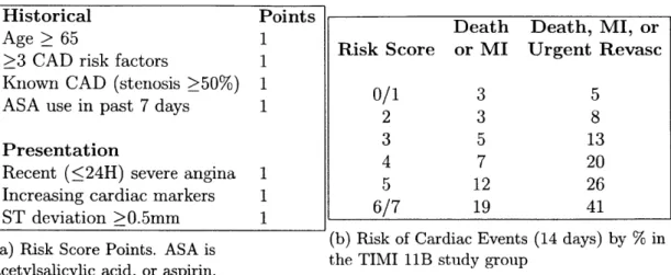
The TIMI risk score is a widely used scoring metric for patient risk stratification post ACS [4]. Separate risk scores exist for STE-ACS and NSTE-ACS. We are only concerned with the NSTE-ACS TIMI score here, as we have a greater need for risk stratification of patients after NSTE-ACS in order to assign appropriate therapies. The scoring criteria and corresponding risk scores for patients post NSTE-ACS are
given in Table 1.1.
Historical Points
Death Death, MI, or
Age > 65 1 Risk Score or MI Urgent Revasc
>3 CAD risk factors 1
Known CAD (stenosis 50%) 1 0/1 3 5
ASA use in past 7 days 1 2 3
8
Presentation 3 5 13
Recent ( 24H) severe angina 1 12 26
Increasing cardiac markers 1
/
12 46ST deviation >0.5mm 1 6/7 19 41
(a) Risk Score Points. ASA is (a) iskScoe Ponts AS isthe (b) Risk of Cardiac Events (14 days) by % inTIMI liB study group acetylsalicylic acid, or aspirin.
Table 1.1: TIMI risk score for UA/NSTEMI.
The TIMI risk score is easy to use for clinicians and easy to understand for pa-tients. Few features are needed to find the TIMI score, and the features used are easily collected. However, it has a limited discriminatory ability for risk stratifica-tion. Previous studies have reported that patients assigned a high-risk TIMI score only account for about 40% of CVDs [6]. Therefore, we desire a risk stratification method with improved discriminatory ability over the TIMI risk score.
1.3
Problem Statement
We believe that machine learning methods can be used to more reliably risk stratify patients when compared with the TIMI risk score. Some work has already been done to determine the efficacy of logistic regression for risk stratification of patients after NSTE-ACS [7]. This work has concluded that logistic regression models, when optimized correctly, can risk stratify patients with a higher discriminatory ability than the TIMI risk score. The TIMI risk score was also initially derived from a logistic regression model [4]. The features that were most predictive of CVD were chosen by examining the weights learned by the logistic regression model. Logistic regression, however, models only one type of relationship between input features and the target variable. Machine learning methods that model other, more complicated,
input-output relationships have not yet been widely applied to risk stratification of patients after ACS. We believe that other types of machine learning models may be able to produce an even more highly discriminatory risk score to be used for risk stratification.
In this thesis, we will analyze the ability of logistic regression, neural networks, and regression trees to risk stratify patients for one-year CVD. We believe that machine learning models can be more effective in risk stratification by modeling more compli-cated relationships between clinical features and outcomes. Various clinical variables that are commonly collected during a post ACS patient's stay in the hospital will be used as our feature set for our machine learning models. These features include many of the factors used to find the TIMI risk score in addition to other features. We will use a feature set including 7 features that are readily apparent for patients after ACS to test our machine learning models. We will also examine using as an augmented feature set including 19 total features. We will be using these machine learning meth-ods to predict likelihood of one-year CVD in each of the patients in our cohort. We will be using one-year CVD likelihood as our risk measure in evaluating the machine learning methods' discriminatory ability over that of the TIMI risk score. We will show that, provided a descriptive feature set, machine learning methods produce risk scores that outperform the discriminatory ability of the TIMI risk score.
Chapter 2
Overview of Machine Learning
Methods
We will be using several types of regression models to calculate risk measures for post ACS patients: logistic regression, neural networks, and regression trees. In this section, we give an overview of the machine learning techniques we will be utilizing. First, we describe logistic regression models. Then, we will summarize neural network models. Lastly, we describe decision tree models.
2.1
Logistic Regression
Logistic regression fits a linear function to the log of the odds of the outcomes, or the logit function. The logit function ensures that the outcomes estimated by the logistic regression model will be constrained to fall between 0 and 1. The relationship is modelled as follows:
N
ln( )=wo + 1 wnzx, (2.1)
n=1
where y is the outcome (in this case, a binary variable representing whether the patient experienced one-year CVD), Xn represents each of the N input features, wn
are the weights learned for each input feature, and wo is a bias term.
that will minimize a loss function. Often, a regularization term is added to the loss function to avoid over-fitting of the function to the data. We make use of L2
normalization, in which the scaled squared magnitude of the weight vector is added to the loss function. Our loss function, L(y, ), is given by
L(y, m) rmin w W + C log(exp(-yi - j) + 1) (2.2)
w,c 2
where P is the number of patients in the training dataset, y, are the actual outcomes,
#j are the estimated outcomes, here CVD, w is the vector of weights found for all
features, and C is a regularization parameter, with larger parameters indicating a weaker L2 regularization, as the error term becomes much stronger relative to the
regularization term with larger C. It should be noted that this loss function works only with class labels of -1 and 1 rather than 0 and 1. For logistic regression, we used
-1 and 1 as class labels rather than 0 and 1.
2.2
Neural Networks
Neural networks are comprised of nodes called neurons arranged in layers. We used a feed-forward, fully connected neural network to estimate a risk score. A feed-forward network is one in which the output of each node is calculated only using information from the previous layer. A fully connected network is one in which all nodes in a layer connect to each node in the following layer. A generalized depiction of a feed-forward, fully connected neural network with N input nodes, one hidden layer, and M nodes in the hidden layer is shown in Figure 2-1.
In this figure, each connection corresponds to a unique weight value. The input nodes pass information to the model, but perform no calculations. In Figure 2-1, each of the N input nodes outputs the value of one of the N features used. The output of the hidden nodes and the output node are nonlinear functions of the linear combination of the weighted outputs of the nodes from the previous layer. These functions are called the activation functions. We have one output node in our model,
Input #1 i W ),' W2x W Input
#2
-.Jw-2
\ M WN2 / Input #N -- W "Input Hidden Output
Layer Layer Layer
Figure 2-1: Neural network model
as we wish to estimate one binary variable, CVD, in the output. In our models, each of the nodes in the hidden layer as well as the output node have a sigmoidal activation function. This function, o, is able to restrict outputs to fall in the range from 0 to 1. The sigmoid function is given as follows:
1
or(a)
= 1,ea'
(2.3)
where a is the weighted sum of the output of the nodes in the previous layer.
Neural networks are optimized using the backpropagation algorithm. When using the backpropagation algorithm, optimal weights are found to minimize a loss function. We use binary cross entropy as the loss function for our neural networks, as we are
estimating a binary target variable. Our loss function, L(y, 9) is given as P
C(y,
)
=-Z
[yi log #j + (1
-
yi) log(1
-
#j)]
(2.4)
i=1
where P is the number of patients in the training dataset, y, are the actual outcomes, and j are the estimated outcomes, here CVD. During backpropagation, errors be-tween the predicted and true outcomes are calculated beginning at the output layer.
Weights from the hidden layer to the output layer are adjusted to minimize the error at the output layer. The error is then calculated at the hidden layer, and weights are again adjusted accordingly. This continues until all weights in the neural net-work have been updated. The netnet-work then updates the predictions using the new weights and repeats the backpropagation process. Backpropagation continues for a set number of epochs, chosen such that the model converges to an optimal solution.
A fully connected, feed-forward neural network with at least three layers (one or
more hidden layers) is also referred to as a multi-layer (ML) perceptron. Accordingly, a feed-forward neural network with no hidden layers is called a single-layer (SL) perceptron. We will use these terms in the remainder of the paper to distinguish between models with one hidden layer and models with no hidden layers.
2.3
Decision Trees
Decision trees use values of the input features to follow a path according to a graph-like model and estimate a target variable. An example of a decision tree regression model with a binary target variable is shown in Figure 2-2. A, B, and C are the input features and Y is the predicted outcome. Decisions are made at each of the nodes using logical relationships on the input features. To make a prediction, we travel through the tree until a leaf, or an outcome node, is reached, where the prediction is assigned. Unlike in neural network models, connections in a decision tree graph do not correspond to weights, but rather to a pathway traveled to reach a leaf. The depth of the tree is equal to the number of decisions that must be made to reach a prediction using the decision tree. The maximum depth of the tree in addition to other parameters must be restricted during training of a decision tree in order to avoid each item in the training dataset having its own leaf in the model.
Decision trees are weak prediction models that often perform worse than neural networks or logistic regression [8]. Decision trees also have a tendency to overfit during the training stage of learning. Multiple methods exist to improve the efficacy of decision tree models.
= 0.1
Node 2 = 1 Node 1Y
=0.75 Node 3 =0 Figure 2-2: Example decision tree model.2.3.1
Gradient Boosted Trees
Gradient boosting is one method that has been successfully used to improve decision tree learning models [8]. Gradient boosting is a type of gradient descent algorithm. Gradient descent algorithms are optimization algorithms in which steps are taken iteratively to minimize a loss function. During each learning step, the algorithm updates the tree model to fit the negative gradient of the loss function. In our gradient boosted tree models, we use mean squared error as the loss function. Our
loss function, L(y, y), is thus given as follows: P
L(y,
= -_) 2, (2.5)i=1
where P is the number of patients in the training dataset, y, are the actual outcomes and #j are the predicted outcomes. First, an initial decision tree model is found. Then, the residuals between the actual outcomes and the predicted outcomes are found. A new decision tree model is found by fitting the tree to the residuals. When using mean squared error as the loss function, the residuals are equal to the negative gradient of the loss function. The tree is updated iteratively for a set number of boosting stages, where at each stage a model is constructed for the residuals arising from the previous stage, chosen such that the model converges to an optimal solution.
2.3.2
Random Forest Trees
Random forest trees also improve on the performance of regular decision trees
[91.
This method makes use of bagging, or bootstrap aggregating, which is when many smaller training sets are chosen randomly from a set of data. Separate trees are trained on each of the random bootstraps. The output is the mean of the predictions output by each of these many decision trees. Random forest trees also make use of feature bagging, in which the feature used to make the decisions at each node are chosen from a random subset of the features. Feature bagging is an effective measure to reduce effects of overfitting, as decision trees choose decisions that separate the training data most decisively. Often, a decision tree may make decisions that split the data well in the first branches of the tree, but the decisions may not result in the most accurate final result. Feature bagging reduces effects of overfitting, especially in the first few stages of the decision tree.
Chapter 3
Results and Discussion
3.1
The MERLIN Dataset
The data for this experiment were collected as part of the MERLIN-TIMI 36 (Metabolic Efficiency with Ranolazine for Less Ischemia in Non-ST-Elevation Acute Coronary Syndrome - Thrombolysis in Myocardial Infarction 36) trial to study the efficacy and safety of the drug ranolazine in reducing ischemia in post NSTE-ACS patients
[10]. This study concluded that ranolazine had no effect on the likelihood of CVD
in post NSTE-ACS patients. Therefore, we are able to use all patient clinical data from this trial to study the discriminatory ability of machine learning methods for risk stratification.
We used two differently sized feature sets to evaluate our models, one with 19 features and the other with 7 features. From the datasets, we created 100 boot-strapped training and testing datasets with 80%/20% training/testing splits. Deaths were stratified among the training and testing datasets. The models were trained on the training sets, and evaluated on the testing sets.
3.1.1
Full Feature Set
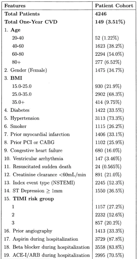
The full set of features used in this study from the MERLIN trial is listed in Table
rather than the TIMI risk score. TIMI risk group 1 includes all patients with a TIMI
risk score from 0-2, TIMI risk group 2 contains those with a risk score from 3-4, and TIMI risk group 3 includes TIMI risk scores from 5-7. All non-binary features were normalized to fall between 0 and 1. Pre-processing steps taken on the feature set are detailed in Appendix A. This feature set is used to evaluate the efficacy of SL and ML perceptrons in addition to logistic regression. As decision tree models are
highly prone to overfitting, the large number of features for the full feature set would
likely lead to overfitting for the tree models. The models would either need to make a large number of decisions to use all the features, resulting in few patients included in each leaf, or not using the entire feature set, which would make it more difficult to compare tree models across bootstraps. Therefore, we do not use the full feature set to evaluate decision tree models.
3.1.2
Reduced Feature Set
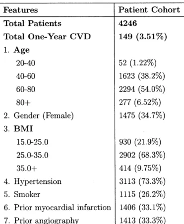
A reduced-size feature set is shown in Table 3.2. This reduced feature set is a subset of
the features shown in Table 3.1. The reduced feature set includes the same patients as the full feature set, but some of their clinical features have been omitted. The reduced feature set contains fewer features than the number used to calculate the TIMI risk score. By limiting the number of features in our feature set, we wish to test if machine learning methods can provide a reliable risk metric when data on a limited number of clinical variables are available. We wish to determine if a small set of highly descriptive features can provide a reliable risk metric for patients. The feature set shown in Table 3.2 is used to evaluate SL perceptron, ML perceptron, logistic regression, decision tree, gradient boosted tree, and random forest tree.
Features Total Patients Total One-Year CVD 1. Age 20-40 40-60 60-80 80+ 2. Gender (Female) 3. BMI 15.0-25.0 25.0-35.0 35.0+ 4. Diabetes 5. Hypertension 6. Smoker
7. Prior myocardial infarction
8. Prior PCI or CABG
9. Congestive heart failure 10. Ventricular arrhythmia 11. Resuscitated sudden death
12. Creatinine clearance <60mL/min
13. Index event type (NSTEMI)
14. ST Depression >
1mm
15. TIMI risk group 1 2 3 16. 17. 18. 19. Prior angiography
Aspirin during hospitalization Beta blocker during hospitalization
ACE-I/ARB during hospitalization
Patient Cohort
4246
149 (3.51%) 52 (1.22%) 1623 (38.2%) 2294 (54.0%) 277 (6.52%) 1475 (34.7%) 930 (21.9%) 2902 (68.3%) 414 (9.75%) 1422 (33.5%) 3113 (73.3%) 1115 (26.2%) 1406 (33.1%) 1102 (25.9%) 680 (16.0%) 147 (3.46%) 24 (0.565%) 891 (21.0%) 2245 (52.3%) 1550 (36.5%) 1157 (27.2%) 2232 (52.6%) 857 (20.2%) 1413 (33.3%) 3729 (87.8%) 3558 (83.8%) 2995 (70.5%)Table 3.1: Baseline characteristics for the patient cohort used in the full feature set. BMI is body mass index; PCI is percutaneous coronary intervention; CABG is coronary artery bypass surgery; ACE-I is angiotensin-converting-enzyme inhibitor; ARB is angiotensin receptor blocker.
Features Patient Cohort Total Patients 4246 Total One-Year CVD 149 (3.51%) 1. Age 20-40 52 (1.22%) 40-60 1623 (38.2%) 60-80 2294 (54.0%) 80+ 277 (6.52%) 2. Gender (Female) 1475 (34.7%) 3. BMI 15.0-25.0 930 (21.9%) 25.0-35.0 2902 (68.3%) 35.0+ 414 (9.75%) 4. Hypertension 3113 (73.3%) 5. Smoker 1115 (26.2%)
6. Prior myocardial infarction 1406 (33.1%)
7. Prior angiography 1413 (33.3%)
3.2
AUC
The area under the curve (AUC) for the receiver operating characteristic (ROC) curve is one metric often used to evaluate the discriminatory ability of machine learning models. The ROC curve is found by plotting the true positive rate of the predictions against the false positive rate. The AUC is then found by computing the area under the ROC curve. An AUC of 1.0 indicates the model is able to perfectly discriminate between high-risk and low-risk patients. An AUC of 0.5 indicates the model is unable to distinguish between high- and low-risk patients. An AUC of 0 means all patients who were high-risk were classified as low-risk and all low-risk patients were found to be high-risk by the model.
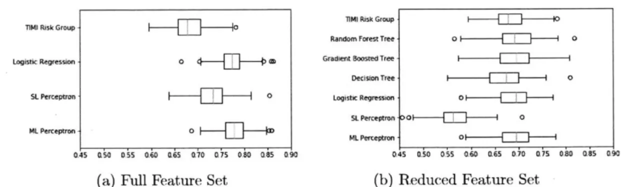
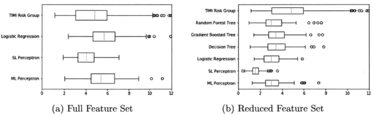
The AUCs for both the full and reduced feature set can be seen in Figure 3-1. These AUCs were calculated on the testing datasets over each of the 100 bootstraps. The mean AUCs and 95% confidence interval (CI) for each of the models are dis-played in Table B. 1 (full feature set) and Table B.2 (reduced feature set) in Appendix B. Figures 3-1a and 3-1b show that the machine learning methods coupled with the augmented feature set are better able than the machine learning methods with the reduced feature to discriminate between high-risk and low-risk patients. Logistic regression and ML perceptron produced the highest median AUC values. SL per-ceptron had a larger median AUC than the TIMI risk group, but produced AUCs lower than ML perceptron and logistic regression. Figure 3-1b shows that most mod-els with the reduced size feature set had comparable AUCs to the TIMI risk group. Logistic regression, ML perceptron, gradient boosted trees, and random forest trees produced results with AUCs slightly higher than the AUCs calculated on the TIMI risk group. Conventional decision tree AUCs were slightly lower than those for the TIMI risk score, and SL perceptron AUCs were quite a bit lower. The AUC values found suggest than ML perceptron and logistic regression produced risk scores with the greatest improvement in discriminatory ability compared to the TIMI risk group. Note in Figure 3.1 that the TIMI risk group, was used as a feature to calculate our risk score. We determined that the addition of the TIMI risk score did not significantly
sTIM Risk Group li1Mi Risk Group
Random Forest Tree 0- 0
Logistic Regression - Gradient Boosted Tree
Decision Tree 0
SL Perceptron 0 Logistic Regression 0
SL Perceptron >O' o
.1-ML Perceptron
- 0
0.45 050 D5 16 6S 070 075 0.80 0.85 090 045 050 055 0.6 065 070 075 OiO 5 090
(a) Full Feature Set (b) Reduced Feature Set
Figure 3-1: AUCs calculated for the testing dataset for each of the 100 bootstraps. The center line in each box represents the median; the box shows the 25th through 75th percentile; the whiskers show the spread out to 1.5*IQR (inter-quartile range, or the difference between the 25th and 75th percentiles) above the 75th percentile; the dots are the outliers.
affect the discriminatory ability of the risk measure we found. Using a feature set that included all features in Table 3.1 but excluding the TIMI risk group, the AUCs changed minimally. For example, with a feature set excluding TIMI risk group, ML
perceptron had an AUC of 0.779 (95% CI [0.772, 0.786]), compared to an AUC of
0.777 (95% CI [0.771, 0.783]) using a feature set that includes the TIMI risk group.
The p-value was 0.0013, indicating these AUCs were not significantly dissimilar. The differences between the AUCs calculated on the training and testing datasets are depicted in Figure 3-2. The median differences for all models for both the reduced and full feature sets range from near 0 to about 0.04, showing that the models are not significantly overfitting to the training sets. When comparing Figure 3-2a with Figure 3-2b, we see that the differences between the AUCs on the training and test-ing datasets for models ustest-ing the reduced dataset have a larger range over the 100 bootstraps than the differences for the models using the augmented feature set. This suggests that with a smaller feature set, discriminatory ability is not as consistent across many bootstraps as the discriminatory ability of models using the full feature set. The test sets for the reduced feature set models produce results with AUCs lower than the AUCs for the training set, suggesting the models are overfitting more often for the reduced data set models than the full feature set models.
Random Forest Tree
Logistic Regression
Gradient Boasted Tree Decision Tree 0 Logistic Regression 5L Perceptron - 0 0 Mt. Perceptron i-V-ML-P-er0n 0 -015 -010 -0.05 100 05 0.10 15 020 -0.15 -010 -0.05 0a Q05 010 a15 02
(a) Full Feature Set (b) Reduced Feature Set
Figure 3-2: AUCt, - AUCte for each of the 100 bootstraps.
3.3
Relative weights of features
3.3.1
Full feature set
A bar graph of the average weights found by the logistic regression model is shown
in Figure 3-3. The feature index labels match the indices for the features in Table
3.1. We see that the weights with the largest magnitudes are indices 1, 9, and 14,
which correspond to age, the presence of congestive heart failure, and ST depression, respectively. This suggests that these three features are the strongest predictors of one-year CVD in this cohort. Age has the largest weight, with a magnitude more than twice that of the next largest weight, corresponding to congestive heart failure. This large weight shows that age is the strongest predictor of one-year CVD in our model. Five of the features have negative weights, suggesting that our model has learned that these features lead to reduced likelihood of CVD in our cohort. The two features with the largest negative magnitude for their weights were prior PCI/CABG and recent aspirin usage. The feature with the smallest weight was diabetes. This suggests our model believes diabetes to be a poor predictor of CVD in this patient cohort.
3.3.2
Reduced feature set
A bar graph of the average weights found by the logistic regression model on the
num-
20.05
-a.5 -0.5I 1 2 3 45 6 7 8 9 10 11 12 13 14 15 16 17 18 19 Feature IndexFigure 3-3: Logistic regression weights for the model trained on the full feature set averaged over 100 bootstraps.
bered features in Table 3.2. As in Figure 3-3, age has the largest weight, suggesting the model has found age to be the strongest predictor of CVD for this cohort. BMI has the next largest weight, and it's negative. The model learned that larger BMIs decrease the risk of CVD. Gender is the smallest weight with a value close to zero. The small weights corresponding to gender in Figures 3-3 and 3-4 show the models have learned that gender is a poor predictor of CVD for this cohort.
3.4
Hazard Ratio
The hazard ratio measures the ratio of the hazard rates in a high risk group to a low risk group [11]. Our hazard ratio is thus defined as follows:
HR =- Rate of CVD for patients in high risk group (3.1) Rate of CVD for patients in low risk group
2-5 2.01.0
-
0.0---0.5
-1.0
I
1 2 3 4 5 6 7 Feature IndexFigure 3-4: Logistic regression weights for the model trained on the reduced feature set averaged over 100 bootstraps.
The hazard ratio is calculated using a Cox proportional hazards model. In our case, the hazard ratio would be the ratio of the rate of CVD in some high risk group compared to the rate in some low risk group. We define the high-risk group as patients with a risk score above the 75th percentile of all risk scores in the patient cohort output by each model and the low-risk group as patients with a risk score below the 75th percentile for the risk score produced by each model. If a model is unable to distinguish between low-risk and high-risk patients reliably, the hazard ratio will be 1. In order for us to say that the hazard ratio is truly above 1, the lower 95% confidence interval must be above 1. A higher hazard ratio means that the model is able to better distinguish between high-risk and low-risk patients.
The hazard ratios calculated on the outputs of the models we tested are shown in Figure 3-5. The mean HRs and 95% CIs for each of the models over the 100 bootstraps are displayed in Table B.3 (full feature set) and Table B.4 (reduced feature set) in Appendix B. Figure 3-5a shows the hazard ratios calculated using the full feature set over the 100 bootstraps. The logistic regression and ML perceptron models on the
full feature set had a higher median hazard ratio than the TIMI risk group, and SL perceptron had a lower median HR. The TIMI risk group had the widest spread in hazard ratios. However, more TIMI risk group HRs were on the higher end of the graph than HRs calculated on the outputs of the machine learning models. Logistic regression models provide results with HRs just as high as the HRs on the TIMI risk group, but with fewer results on the high end of the spread of HRs. Figure 3-5b shows the HRs using the reduced size feature set. The median HR using the TIMI risk group was higher than the median HR for all of the machine learning models for the reduced feature set. The TIMI risk group had HRs of up to 12, while the machine learning models trained on the reduced size feature set only had HRs reaching as high as 8. The SL perceptron method produced outputs with particularly low HRs. Some HRs went even lower than 1, indicating the SL perceptron produced results placing a higher rate of risk in the group determined to be low risk. ML perceptron, logistic regression, and the decision tree models for the reduced feature set all produced HR results with a similar median and spread.
II RikGoup 00l]---~ a14 i Gop I0
Random Forest Tree - 0000 Logistic Regression 0 C Gradient Boosted Tree 0 00
Decision Tree CO 0
SL Perceptron Logistic Regression - o
SL Perceptron o-F - 0
ML Perceptron I-.-.--L 0 Per--ptrJn o0 0
0 2 4 6 5 10 12 0 2 3
5 1 12
(a) Full Feature Set (b) Reduced Feature Set
Figure 3-5: Hazard ratios calculated for the testing dataset for each of the 100 boot-straps.
3.5
Net Reclassification Improvement
The Net Reclassification Improvement (NRI) measures the added usefulness of a newer model over an older one. The NRI has previously been successfully applied to risk stratification models [121. Multiple variations in the definition of the NRI exist.
We make use of the two-category NRI in the evaluation of our models because we are analyzing a binary target variable. The two-category NRI is formulated as a linear combination of probabilities and is defined as follows:
NRI = P(upevent) - P(downlevent)
+
P(downnon - event) - P(uplnon - event),(3.2)
where the 'event' indicates CVD occurred, 'non-event' means the patient did not experience CVD, 'up' indicates the old model characterized the patient in the low risk group while the new model placed the patient in the high risk group, and 'down' indicates the old model characterized the patient as high risk while the new model characterizes as low risk. For example, an NRI of zero indicates the new model had the same discriminatory ability as the old model. A negative NRI indicates the new model was not able to discriminate between low-risk and high-risk as well as the old model, and a positive NRI shows the new model discriminated more accurately than the old model. The NRI ranges from -2 to 2. An NRI of 2 indicates the old model classified no patients correctly, while the new model was able to discriminate correctly between all high-risk and low-risk patients. An NRI of -2 indicates the new model classified none of the patients correctly, but the old model identified all high- and low-risk patients correctly.
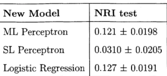
The NRIs showing the improvement of each of our models for the full feature set over the TIMI risk group are shown in Table 3.3. Table 3.4 shows the NRIs for models used with the reduced feature set compared with the TIMI risk group. Both the mean NRI and the 95% CI are shown. When calculating each of these NRIs, the TIMI risk group was the old model. The new models are given in the tables. The NRIs found using the predicted outcomes on the test dataset are shown in both tables. The testing dataset NRIs for the machine learning models with the augmented feature set are positive and with CIs that do not overlap zero. This shows that the machine learning models with a larger set of features exhibit heightened discriminatory ability over the TIMI risk group. The logistic regression and ML perceptron showed a larger
New Model NRI test ML Perceptron 0.121 t 0.0198
SL Perceptron 0.0310 t 0.0205
Logistic Regression 0.127 t 0.0191
Table 3.3: Mean NRIs and 95% CIs for various models and the full feature set com-pared with the TIMI score
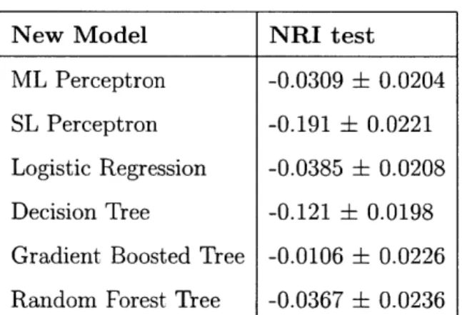
improvement over the TIMI dataset. Both models had a mean NRI around 0.12 over 100 bootstraps with the full feature set. SL perceptron, however, showed poorer performance. The lower bound of the 95% CI was about 0.01, not much larger than zero. However, the 95% CI is still positive, indicating with a high likelihood that SL perceptron exhibits a higher discriminatory ability than the TIMI risk score. The mean NRIs on the testing datasets for each of the models with the reduced feature set were negative. This suggests that the models paired with the reduced size feature set had poorer discriminatory ability than the TIMI risk group. Additionally, only the confidence interval for the gradient boosted decision tree overlapped with zero. The CIs below zero suggest that the results using the machine learning models with the reduced feature set had significantly worse discriminatory ability than the TIMI risk group. SL perceptron had the worst discriminatory ability compared with the TIMI risk score, with an NRI of -0.191 (95% CI [-0.0221, -0.169]).
More NRIs comparing machine models with each other are shown in Table B.5 (full feature set) and Table B.6 (reduced feature set). The very small mean NRI comparing the logistic regression and ML perceptron results for the full feature set, especially compared with the size of the CI, indicate that for the full feature set, logistic regression and ML perceptron have similar discriminatory ability for risk stratification.
Table 3.4: Mean NRIs and 95% CIs for various models and the reduced feature set
compared with the TIMI score
New Model NRI test
ML Perceptron -0.0309 0.0204
SL Perceptron -0.191 0.0221
Logistic Regression -0.0385 0.0208
Decision Tree -0.121 0.0198
Gradient Boosted Tree -0.0106 0.0226
Chapter 4
Conclusions and Future Work
The results in the previous chapter suggest that machine learning methods can pro-duce a risk score with a greater discriminatory ability than that of the TIMI risk score, but only if a more descriptive set of features is available than those used to calculate the TIMI risk score. If only a small number of features is available, the machine learning methods produce a risk metric with a discriminatory ability similar to that of the TIMI risk group. Both ML perceptron and logistic regression offer im-proved discriminatory ability using the full feature set. Using the full feature set, SL perceptron does not discriminate between high- and low-risk patients as well as ML perceptron or logistic regression, but SL perceptron still produces a risk score with higher discriminatory ability than the TIMI risk score. Using the reduced size feature set, the ML perceptron, logistic regression, decision tree, gradient boosted tree, and random forest tree models exhibited discriminatory ability a bit worse than that of the TIMI risk group. Each of these models produced average AUCs that were slightly higher than those found for the TIMI risk group, but the NRIs for each of these mod-els when compared with the TIMI risk score were slightly negative. The HRs for the machine learning models were worse than those for the TIMI risk group. The con-flicting results of the performance metrics make it difficult to determine if the models other than SL perceptron used with the reduced size feature set produced slightly improved or slightly worsened risk metrics compared with the TIMI risk group. How-ever, with the reduced size feature set, SL perceptron performs consistently worse
than the TIMI risk group when evaluated using the AUC, HR, and NRI. Out of all models evaluated, ML perceptron and logistic regression paired with the full feature set produced the risk score that had the highest discriminatory ability.
Our results indicate that a more descriptive feature set could improve the results of the machine learning methods. We found the performance of machine learning methods using the full feature set improved, but little or no improvement using the reduced feature set. Therefore, it seems that the features are primarily responsible for the improved performance, not the models used. Additionally, ML perceptron and logistic regression had similar discriminatory ability, although ML perceptrons are able to model much more complicated relationships than logistic regression models. Future work should include an investigation of the proper features to use with machine learning methods to improve the overall performance. Some features that were not included in this study may be highly predictive of CVD. For instance, our reduced feature set did not include all data used to calculate the TIMI risk score. In order to compare the discriminatory ability of the TIMI risk score with that of machine learning methods more directly, machine learning methods must be tested using a feature set that is the same as the feature set used to find the TIMI risk score. Additionally, we only compared our results with the TIMI risk group, rather than TIMI risk score, because of lack of data for the TIMI risk score for our patients. For
a more accurate comparison, we need data on the TIMI risk score.
Other datasets could provide a larger feature set and larger patient cohort to test the efficacy of additional features in providing a risk score. However, as the size of the feature set relative to the size of the patient cohort increases, the risk of overfitting to the feature set increases accordingly [7]. The larger the feature set becomes, the larger the size our dataset must be in order to avoid overfitting. Therefore, in order to avoid overfitting with a larger number of features, we must collect data on a larger number of patients. The GRACE dataset contains a larger patient population and feature set than the MERLIN dataset; the GRACE dataset contains tens of thousands of patients, hundreds of features, and many long-term and short-term outcomes [5]. Our dataset also only included 149 CVDs; a dataset including more patient deaths, such
as the GRACE dataset, may improve the ability of the machine learning methods to be accurately trained. Studying the usefulness of models trained using larger numbers of features and patients might be a promising future direction. The GRACE dataset could be one useful source of data for studies using machine learning models applied to new features not included in this study.
Previous work has included applying machine learning algorithms to features ex-tracted from a patient's ECG [6]. This work has shown that ECG-morphology based risk metrics can be used to identify some patients that are generally classified as low-to moderate-risk using only patient record risk features. Creating a feature set that combines ECG features with patient record features could increase the discrimina-tory ability of machine learning models by allowing us to reliably identify a larger number of high-risk patients. Our feature sets in Figure 3.1 and Figure 3.2 included a binary variable indicating whether ST depression was present in the patient's ECG. However, more information may be extracted from the ECG that might improve the discriminatory ability of these algorithms. For example, the level of ST depression was not included in our models for this thesis. ECG data and patient record data combined could allow us to create even more powerful models for risk stratification.
Other machine learning methods may also be applicable to risk stratification mod-els. The decision tree models applied in this paper were all regression trees; they were able to output risk measures that fell between 0 and 1. Their outputs were a pre-diction that was the average value of the outcomes included in the patients in each leaf. Classification trees could also be easily applied to our problem. Classification trees output a prediction of the class of a patient. In this case, we have two output classes, high-risk or low-risk. The classification trees would predict whether each pa-tient would experience one-year CVD, and this prediction would serve as their risk class. Another classification method that may be applicable to risk stratification is a support vector machine (SVM). SVMs find a decision boundary in multidimensional space between two classes of objects and predict the side of the decision boundary on which each patient falls by calculating a linear combination of the patient's fea-tures. As we have two classes in our problem, SVMs are applicable. Although it is
a classification algorithm, higher granularity of the risk measure prediction may be found by finding an input's distance from the decision boundary. Different decision boundaries can be used when implementing an SVM. Decision boundaries may be linear or kernelized.
Risk stratification has many applications in healthcare, from deciding who should be serviced in the emergency room first to assigning therapies for a number of diseases other than ACS, such as diabetes and cancer. When a model is trained, it does not need to be trained again. Once a reliable model is found, it can be used repeatedly to find a risk measure by providing the model with the necessary features. Machine learning methods' successful application to ACS suggests a hopeful outlook for those looking to apply machine learning to risk stratification for other ailments. Machine learning models could help doctors to enhance their discriminatory ability when risk stratifying patients, allowing them to provide more targeted therapies and assess each patient's needs.
Appendix A
Materials and Methods
A. 1
Pre-processing
The original MERLIN dataset included 4395 patients and three features in addition to those listed in Table 3.1. 'Age > 75' was a binary feature included in the original
MERLIN dataset. It was removed due to it being repetitive, as raw age was already a feature included in the set. 'Left ventricular ejection fraction' was also removed due to it missing values for about a third of the patients. Additionally, 'Patient ID' was removed, as it gives no clinical information about the patients, but rather functions as an identifier. Lastly, patients were removed from the dataset who were missing entries for any of the remaining features. This step removed 149 patients from the dataset. Before running the machine learning algorithms, the dataset was divided into training and testing datasets with an 80%/20% split with deaths stratified among the training and testing sets. 100 bootstraps of the training and testing datasets were found, and the machine learning algorithms were trained on each of the bootstrapped training sets separately. We also created the list representing the target outcomes, one-year
CVD. We were provided with information on the number of days CVD occurred after
the patient checked into the hospital and a binary variable on whether the patient experienced CVD. Pre-processing was needed to obtain an outcome variable for one-year CVD. This was obtained by examining whether the patient's CVD occurred within 365 days of hospital admittance for ACS.
A.2
Code
Code for this project was written in both Python and MATLAB.
The neural network models were written using Keras in Python [13]. Models for the reduced feature set and augmented feature set were optimized separately using a grid search. Both the full and reduced feature set ML perceptrons had 25 nodes in the hidden layer and a batch size of 2'. The full feature set ML perceptron was run for 200 epochs, while the reduced feature set model was run for 240 epochs. The SL perceptrons was run with a batch size of 2' for both the full and reduced size datasets. The SL perceptron was run for 200 epochs for the full size feature set and 240 epochs for the smaller feature set. Both L, and L2 regularization were used concurrently
for the SL perceptron. Regularization parameters were optimized by a grid search, which found the optimal parameter values to be A, = 10-' and A2 = 10 . The loss
function used was binary cross entropy.
The logistic regression and decision tree models were created using scikit-learn in Python [14]. Multple parameters were optimized using a grid search, training on each of the training sets and finding predictions on each of the testing datasets. The logistic regression models were run on both the full and reduced feature sets with L2
regularization and a A of 10'. The regular decision tree was run with a minimum of 1024 samples per split, a minimum of 256 samples per leaf, and a maximum depth of 6. The gradient boosted tree was run with a minimum of 512 samples per split, a minimum of 128 samples per leaf, a maximum depth of 2, and a learning rate of 0.01. The random forest tree had a minimum of 1024 samples per split, a minimum of 128 samples per leaf, and a maximum depth of 6.
Appendix B
Tables
Model AUC test
TIMI Risk Group 0.680 0.00784
ML Perceptron 0.777 t 0.00639
SL Perceptron 0.730 0.00727
Logistic Regression 0.771 0.00670
Table B.1: AUCs calculated on the testing dataset for various models on the full feature set.
Model AUC test
TIMI Risk Group 0.680 + 0.00784
ML Perceptron 0.690 + 0.00828
SL Perceptron 0.630 + 0.0110
Logistic Regression 0.691 0.00860
Decision Tree 0.679 0.00816
Gradient Boosted Tree 0.700 + 0.00830
Random Forest Tree 0.693 0.00842
Table B.2: AUCs calculated on the testing dataset for various models on the reduced feature set.
Model HR test
TIMI Risk Group 4.54 0.565
ML Perceptron 7.88 0.328
SL Perceptron 5.42 0.307
Logistic Regression 4.61 0.283
Table B.3: HRs calculated on the testing dataset for models on the full feature set.
Table B.4: HRs calculated on the testing dataset for models set.
on the reduced feature
Old Model New Model NRI test
LogReg SKLearn Neural network 0.0066 + 0.00887
Table B.5: Net reclassification index and 95% confidence interval for models using on the full feature set.
Table B.6: Net reclassification index and 95% confidence the reduced feature set.
interval for models using on
Model HR test
ML Perceptron 3.45 0.233
SL Perceptron 3.49 + 0.249
Logistic Regression 2.18 0.147
Decision Tree 3.71 0.268
Gradient Boosted Tree 3.77 0.267
Random Forest Tree 3.52 t 0.271
Old Model New Model NRI test
LogReg SKLearn Neural network 0.000648 0.0724
Neural network Gradient Boosted Tree -0.0180 0.149
Decision Tree Gradient Boosted Tree -0.0822 0.133
Gradient Boosted Tree Random Forest Tree 0.0316 0.137
Appendix C
Figures
j 4
(a) Full Feature Set
llMaaask GMu 0 a
Random Forest Tree - - o
Gadient Boosted Tree - aD
Decision Tree i-- - O
Logistic Reression - I -
---SL Perceptron 0 00
Mt Perceptron O 0w0
(b) Reduced Feature Set Figure C-1: HRt,/HRte for each of the 100 bootstraps.
TIMI Risk Group
Logistic Regression SL Perceptron ML. Perceptron
000 0
0 00
0
00 00 CO 0 i 0 00 0 C 00 0 0 0 0 0 4Bibliography
[1] E. Benjamin, S. S. Virani, C. W. Callaway, A. Chang, S. Cheng, S. Chiuve,
M. Cushman, F. Delling, R. Deo, S. D. de Ferranti, J. F. Ferguson, M. Fornage,
C. Gillespie, C. Isasi, M. Jimenez, L. Chaffin Jordan, S. E. Judd, D. Lackland,
J. Lichtman, and P. Muntner, "Heart disease and stroke statistics2018 update: A
report from the american heart association," vol. 137, p. CIR.0000000000000558,
01 2018.
[2] E. A. Amsterdam, N. K. Wenger, R. G. Brindis, D. E. Casey, T. G. Ganiats,
D. R. Holmes, A. S. Jaffe, H. Jneid, R. F. Kelly, M. C. Kontos, G. N. Levine,
P. R. Liebson, D. Mukherjee, E. D. Peterson, M. S. Sabatine, R. W. Smalling,
and S. J. Zieman, "2014 aha/ace guideline for the management of patients with non-st-elevation acute coronary syndromes," Circulation, 2014.
[3] H. Chang, J. K. Min, S. V. Rao, M. R. Patel, 0. P. Simonetti, G. Ambrosio,
and S. V. Raman, "Non-st-segment elevation acute coronary syndromes,"
Cir-culation: Cardiovascular Imaging, vol. 5, no. 4, pp. 536-546, 2012.
[4] A. EM, C. M, B. PM, and et al, "The timi risk score for unstable angina/nonst elevation mi: A method for prognostication and therapeutic decision making,"
JAMA, vol. 284, no. 7, pp. 835-842, 2000.
[5] K. A. A. Fox, 0. H. Dabbous, R. J. Goldberg, K. S. Pieper, K. A. Eagle, F. Van de
Werf, A. Avezum, S. G. Goodman, M. D. Flather, F. A. Anderson, and C. B. Granger, "Prediction of risk of death and myocardial infarction in the six months after presentation with acute coronary syndrome: prospective multinational ob-servational study (grace)," BMJ, vol. 333, no. 7578, p. 1091, 2006.
[6] Y. Liu, Z. Syed, B. M. Scirica, D. A. Morrow, J. V. Guttag, and C. M. Stultz,
"Ecg morphological variability in beat space for risk stratification after acute coronary syndrome," Journal of the American Heart Association, vol. 3, no. 3,
2014.
[7] M. Pavlou, G. Ambler, S. R. Seaman, 0. Guttmann, P. Elliott, M. King, and
R. Z. Omar, "How to develop a more accurate risk prediction model when there are few events," BMJ, vol. 351, 2015.
[8] A. Natekin and A. Knoll, "Gradient boosting machines, a tutorial," vol. 7, p. 21,
[9] L. Breiman, "Random forests," Machine Learning, vol. 45, pp. 5-32, Oct 2001. [10] D. A. Morrow, "Effects of ranolazine on recurrent cardiovascular events in
pa-tients with nonst-elevation acute coronary syndromesthe merlin-timi 36
random-ized trial," Jama, vol. 297, no. 16, p. 1775, 2007.
[11] D. R. Cox, "Regression models and life-tables," Journal of the Royal Statistical
Society. Series B (Methodological), vol. 34, no. 2, pp. 187-220, 1972.
[12] M. Pencina, R. D'Agostino, and E. Steyerberg, "Extensions of net reclassifica-tion improvement calculareclassifica-tions to measure uefulness of new biomarkers," vol. 30,
pp. 11-21, 01 2011.
[13] F. Chollet et al., "Keras." https://keras.io, 2015.
[14] F. Pedregosa, G. Varoquaux, A. Gramfort, V. Michel, B. Thirion, 0. Grisel, M. Blondel, P. Prettenhofer, R. Weiss, V. Dubourg, J. Vanderplas, A.
Pas-sos, D. Cournapeau, M. Brucher, M. Perrot, and E. Duchesnay, "Scikit-learn:
Machine learning in Python," Journal of Machine Learning Research, vol. 12,