HAL Id: hal-02907937
https://hal.archives-ouvertes.fr/hal-02907937
Submitted on 27 Jul 2020
HAL is a multi-disciplinary open access
archive for the deposit and dissemination of
sci-entific research documents, whether they are
pub-lished or not. The documents may come from
teaching and research institutions in France or
abroad, or from public or private research centers.
L’archive ouverte pluridisciplinaire HAL, est
destinée au dépôt et à la diffusion de documents
scientifiques de niveau recherche, publiés ou non,
émanant des établissements d’enseignement et de
recherche français ou étrangers, des laboratoires
publics ou privés.
Neural networks based speed-torque estimators for
induction motors and performance metrics
Sagar Verma, Nicolas Henwood, Marc Castella, Al Jebai, Jean-Christophe
Pesquet
To cite this version:
Sagar Verma, Nicolas Henwood, Marc Castella, Al Jebai, Jean-Christophe Pesquet. Neural networks
based speed-torque estimators for induction motors and performance metrics. IECON 2020 - 46th
Annual Conference of the IEEE Industrial Electronics Society, Oct 2020, Singapore, Singapore.
pp.495-500, �10.1109/IECON43393.2020.9255236�. �hal-02907937�
Neural Networks based Speed-Torque Estimators
for Induction Motors and Performance Metrics
Sagar Verma,
1,2Nicolas Henwood,
2Marc Castella,
3Al Kassem Jebai,
2Jean-Christophe Pesquet,
11
Universit´e Paris-Saclay, CentraleSup´elec, Inria, Centre de Vision Num´erique
2Schneider Toshiba Inverter Europe
3
SAMOVAR, T´el´ecom SudParis, Institut Polytechnique de Paris
Abstract—This paper focuses on the quantitative analysis of deep neural networks used in data-driven modeling of induction motor dynamics. With the availability of a large amount of data generated by industrial sensor networks, it is now possible to train deep neural networks. Recently researchers have started exploring the usage of such networks for physics modeling, online control, monitoring, and fault prediction in induction motor operations. We consider the problem of estimating speed and torque from currents and voltages of an induction motor. Neural networks provide quite good performance for this task when analysed from a machine learning perspective using standard metrics. We show, however, that there are some caveats in using machine learning metrics to analyze a neural network model when applied to induction motor problems. Given the mission-critical nature of induction motor operations, the performance of neural networks has to be validated from an electrical engineering point of view. To this end, we evaluate several traditional neural network architectures and recent state of the art architectures on dynamic and quasi-static benchmarks using electrical engineering metrics.
Index Terms—induction motor, neural networks, deep learning, time series, training
I. INTRODUCTION
Induction motors have very complex dynamics and it is essential to have a controller that can provide robust control based on these dynamics. Induction motor controllers also offer protection and supervision of the electro-mechanical system [1], [2]. For these services, it is mandatory to know the dynamical physical model of induction motors. Accurate dynamics is derived from the first principles of physics. These dynamical models are dependent on different induction motor physical characteristics like currents, voltages, speed, fluxes, inductances, and resistances, which are measured directly or indirectly using sensors or estimators. Accurately measuring some of these quantities is challenging due to the presence of noise and the operating conditions.
Controllers derived from physical models are widely used in industry and are very reliable. Although moderate complexity models of the induction motor exist, they are nonlinear and include several uncertain parameters. Industrial Internet of Things (IIoT) has made it possible to collect a large amount of data from different electro-mechanical devices. This collection of real-time or near real-time data from induction motor systems has enabled the development of online decision
algo-rithms for electrical system monitoring applications. Recent advances in deep neural networks for time series analysis have also led to better prediction models. End-to-end learning of temporal dynamics from time-series data has been made easier due to techniques like Convolutional Neural Network (CNN), Recurrent Neural Network (RNN), and Long-Short Term Memory (LSTM) structures.
Neural networks have been actively used for controller [3]–[5], monitoring and fault prediction in electrical motor operations [6]–[9]. Verma et. al. [10] used encoder-decoder architecture to learn dynamics from induction motor signals. These methods are evaluated using machine learning metrics like mean square error, r-square, accuracy, etc. These metrics are well suited for regression and prediction tasks but have an inherent bias towards the dataset. We analyze how and when these metrics fail and propose a way to properly evaluate neural network methods for induction motor problems using dynamic and quasi-static benchmarks, as well as electrical engineering metrics. We consider the problem of predicting speed and electromagnetic torque from currents and voltages represented in (d − q) frame. We experiment on network architectures similar to those proposed in [10].
This paper is structured as follows: Section II provides a short survey on induction motor physics modeling and neural networks. Section III explains the nonlinear physical model of an induction motor and electrical engineering metrics used in our experiments. Section IV details neural network models used in this paper. Section V describes the training and benchmark data. Section VI contains experimental details and the obtained results. In the last section, conclusions are drawn and some possible extensions of this work are mentioned.
II. RELATEDWORK
Development in model-based nonlinear control methods in the last three decades can be grouped in the following cate-gories: feedback linearization methods [11], [12], Lyapunov-based control [13], [14], and passivity-Lyapunov-based methods [15], [16]. The state-space model of an induction motor is described in [17]. Modeling of electrical motors based on analytical mechanics and energy consumption is presented in [18]. Existing methods for designing a controller for an induction motor can be done in two ways, when perfect knowledge of
the parameters is available [19]–[21] and when there is an uncertainty associated with the estimation of the parameters [22]–[24]. Model-based control methods for induction motors all require proper knowledge about four independent electrical parameters of the motors.
Neural network-based control methods have also been pro-posed to learn a better model that can overcome problems associated with the traditional model-based approach. [25] uses radial basis neural networks to learn the relationship be-tween currents and flux linkages. [6] presents a neural network classifier for fault diagnosis in electrical motor operations. The approach does not use dynamics modeling and only relies on supervised labels [8], learn motor dynamics from simulated data, and perform fault detection in simulated motor operations. In [10], encoder-decoder network is proposed to learn dynamics of electrical motor directly from recorded data. The proposed method achieves good performance in modeling the input-output relationship.
The reasons why neural networks fail is analyzed in [26]. Neural networks make fewer assumptions, have a large number of parameters, and have different modeling processes, open-ing more possibilities for inappropriate uses and problematic applications. Another major pitfall consists of treating neural networks as black boxes. In [27] a robustification technique is proposed to interpret neural network results in terms of the input effects and interactions among input variables. Underfitting and overfitting being well-known problems in machine learning methods, neural networks are prone to these problems due to their data-hungry nature and large number of parameters, as discussed in [28].
III. PHYSICALMODELING
A. Nonlinear State-Space Motor Model
In this section, we present the mathematical model of an induction motor we consider, which was introduced in [17].
Rotating reference frame at pulsation ωs (d − q model) is
used to express all the quantities. Park transformation is used to convert the quantities from the fixed three-axis frame to the orthogonal rotating (d − q) frame. The fifth-order nonlinear state space model of the induction motor reads as follows:
J np d dtωr= 3 2np=(ψ ∗ sis) − τL (1) d dtψs= −jωsψs− Rsis+ us (2) d dtψr= −jωsψr− Rrir+ jωrψr (3)
where =(z) and z∗ are respectively the imaginary part and
conjugate of z. np denotes the number of pole pairs, J the
motor shaft inertia, τL the load torque, and us= usd+ jusq
the motor input voltage in the (d − q) frame. ωr (np times
the mechanical speed), ψs = ψsd+ jψsq (stator flux), and
ψr= ψrd+ jψrq (rotor flux) are the five state variables. The
flux variables are linked to the current variables is(stator) and
ir(rotor) by nonlinear relationships [29] given by :
ψs= Lf sis+ Lm(is+ ir) 1 + γ|is+ ir| ψr= Lf rir+ Lm(is+ ir) 1 + γ|is+ ir| (4)
The parameters are the stator and rotor resistances Rs and
Rr, the stator and rotor leakage inductances Lf sand Lf r, and
the magnetic saturation coupling parameters Lm and γ.
B. Performance Metrics
To evaluate neural networks we use electrical engineering (EE) performance metrics widely used in industrial settings. We report the following metrics, applied to the response signal to a speed or torque reference ramp (whose amplitude is the absolute difference between the starting and target values):
• 2% response time (t2%) is the time value at which the
response signal has covered 2% of the ramp amplitude.
• 95% response time (t95%) is the time value after which
the response signal remains at less than 5% of the ramp amplitude from the target value.
• Overshoot (D%) is the difference between the maximum
peak value of the response signal and the target value. It is expressed in percentage of the ramp amplitude.
• Steady-state error (Ess) is the difference between the
response signal and target values once the steady-state has been reached.
• Following error (Ef ol) is the difference between the
reference and response signal values at the time when the reference value has covered 50% of the ramp amplitude.
• Maximum acceleration torque (for speed ramp only)
(∆τmax) is the maximum response torque deviation
dur-ing the speed ramp.
• Speed drop (for torque ramp only) (SD) is the
maxi-mum response speed deviation during the torque ramp.
IV. DATADRIVENMODELING
A. Standard Neural Networks
We use three benchmark neural network architectures from [10] for our experiments. Since the focus of this paper is on the evaluation of performance metrics, we only use subset of benchmark networks from [10].
1) Four layer Fully Connected Network (FCN): A four
layer fully connected network which has been used in different tasks related to induction motor operations.
2) Two layer Long-Short Term Memory Network (LSTM):
In sequential neural networks, we use LSTM as it performs better than RNN. We use two layers of LSTM, followed by three fully connected layers in this network.
3) Four layer Convolutional Neural Network (CNN):
CNNs have been shown to provide competitive results on sequential data. In line with recent advances in the use of 1D convolutions for sequential tasks, we also employ a four-layer convolutional neural network for our experiments.
B. Encoder-Decoder Networks
Encoder-decoder networks have been proven to perform better when input and output dimensions are the same. We con-sider encoder-decoder variants proposed in [10]. This structure consists of encoding and decoding blocks with convolutional and deconvolutional layers, respectively.
1) Vanilla Encoder-Decoder (Vanilla): Vanilla
Encoder-Decoder consists of four layers of convolutional and four layers of a deconvolutional block.
2) Skip Connections (Skip): We add skip connections to
each convolutional layer of the encoding block to consecutive deconvolutional layer of the decoder block.
3) Recurrent Skip Connections (RNN): Better temporal
dynamics learning is achieved by introducing RNN layers in skip connections.
4) Bidirectional Recurrent Skip Connections (BiRNN):
Bidirectional RNN in skip connections have a better scope over complete input sequence than unidirectional RNN.
5) Bidirectional Diagonalized Recurrent Skip Connections (BiDiagRNN): RNNs in the network are diagonalized by making their parameters independent of each other. This leads to fewer parameters.
C. Loss Function and Evaluation Metrics
Very often, mean square error loss is used to train a regression model. Total variation weighted mean square loss LTV-MSE as proposed in [10] gives more weight to dynamic
parts of the signal:
LTV-MSE= 1 N N X i=1 T −1 X t=1 |yi t− y i t+1| ! | {z } Total Variation MSE z }| { 1 T T X t=1 (yti− ˆyti)2 ! (5) where yi
tand ˆyitare the values of output and predicted sample
i at time-step t, respectively. N is the number of training samples where each sample is of duration T .
To analyse model performance at global scope, we report machine learning (ML) metrics. Mean absolute error (MAE), symmetric mean absolute percentage error (SMAPE), and
coefficient of determination (R2) are used, whose expressions
are recalled below:
MAE(y, ˆy) = 1 T T X t=1 |yt− ˆyt| (6) SMAPE(y, ˆy) = 100 T T X t=1 |ˆyt− yt| |ˆyt| + |yt| (7) R2(y, ˆy) = 1 − PT t=1(ˆyt− ¯y)2 PT t=1(yt− ¯y)2 (8)
where ytis the ground truth, ˆytis the predicted output of the
model at time t, and T is the total experiment duration. ¯y
denotes the mean of ground truth y.
V. DATASETS
We use the motor model proposed in [17] to generate our simulated data.
A. Reference Trajectory Generator
To generate simulated training and validation sets, we created a trajectory generator that generates realistic reference speed and load torque trajectories. For every simulation, the number of static states is drawn randomly from a uniform distribution between 5 and 15. The duration of a static state in a simulation is drawn from a uniform distribution between 1 and 5 seconds. Ramp duration between two consecutive static states is generated according to a shifted truncated exponential distribution between 4 and 2000 milliseconds to provide more frequent short duration ramps. For each static state, speed and load torque values are generated according to a uniform distribution on [-70, 70] Hz and [-120, 120] %
of nominal torque (%τnom), respectively. Figure 1 shows a
sample reference trajectory from the training set.
0 20 40 60 80 Time (s) 130 75 0 75 130 Load Torque (% Nominal Torque) 0 20 40 60 80 Time (s) 80 40 0 40 80 Reference Speed (Hz)
Fig. 1: Reference speed and load torque trajectories from one of the training samples.
B. Training and Validation Dataset
75 50 25 0 25 50 75 Reference Speed (Hz) 150 100 50 0 50 100 150
Load Torque (% of Nominal Torque)
(a) Training zone
100 75 50 25 0 25 50 75 100 Reference Speed (Hz) 150 100 50 0 50 100 150
Load Torque (% of Nominal Torque)
(b) Validation zone Fig. 2: Density plots of torque vs speed plans for all the simulations in training set and validation set.
We use our reference trajectory generator to generate 100 simulated paths totaling about 1000 speed and torque ramps in 150 minutes for the training set and 50 simulations totaling
about 200 ramps in 30 minutes for the validation set. Torque-speed plan density plots for training and validation zones are shown in Figure 2. We then simulate these trajectories using our Simulink model of a 4kW induction motor and collect simulation data every 4ms. The simulation dataset consists
of the following electrical quantities: currents isd and isq,
voltages usd and usq acting as inputs and rotor speed ωr,
and electromagnetic torque τem acting as outputs.
C. Test Dataset
The validation dataset is sufficient to evaluate neural net-work models on ML metrics (equations (6), (7), and (8)). To properly evaluate neural network models on EE performance metrics (see Section III-B), we generate five classical bench-mark trajectories. These are divided into two categories:
1) Quasi-Static Benchmarks: At constant torque, reference
speed goes from 70 to -70Hz in 50 seconds. Two constant torques are tested: no-load and 50% of the nominal load. We name these benchmarks, Quasi-Static1 and Quasi-Static2, respectively. In the case of the 50% nominal load torque, the torque has already reached the steady-state before the start of the benchmark.
2) Dynamic Benchmarks: We generate three dynamic
benchmarks to evaluate our neural network models:
(a) Dynamic-Speed1: Reference speed goes from 0 to 50Hz in 1 second at no load.
(b) Dynamic-Speed2: Reference speed goes from 50 to -50Hz in 1 second at 50% of nominal load.
(c) Dynamic-Torque: Load torque goes from 0 to 100% of nominal torque in 4ms with a constant 25Hz refer-ence speed.
VI. EXPERIMENTALRESULTS
Model Speed (ωr) Torque (τem)
MAE SMAPE MAE SMAPE
FCN 0.79 21.77% 0.57 48.66% LSTM 0.11 18.76% 0.21 43.01% CNN 0.06 19.14% 0.09 38.91% Vanilla 0.05 18.94% 0.10 39.91% Skip 0.08 19.08% 0.12 43.23% RNN 0.06 19.31% 0.08 41.81% BiRNN 0.05 18.67% 0.09 42.82% DiagBiRNN 0.03 18.76% 0.04 38.46% R2is 0.99 for all the networks for both quantities.
TABLE I: ML metrics for the predictions done on benchmark set using standard models and the encoder-decoder variants. Aggregated results are shown for all 5 benchmarks.
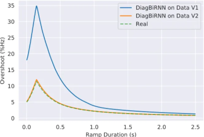
During our experiments, we found that all our models were biased towards long-duration ramps present in the training data. This was due to the fact that when reference trajectories were generated, ramp durations were originally sampled from a uniform distribution. Motor responses to ramps being far more different for a small ramp duration variation when the ramps are short than when they are long, a uniform distribution was not adequate. To overcome this bias, generating data
0.0 0.5 1.0 1.5 2.0 2.5 Ramp Duration (s) 0 5 10 15 20 25 30 35 Overshoot (%Hz) DiagBiRNN on Data V1 DiagBiRNN on Data V2 Real
Fig. 3: Overshoot vs. ramp for DiagBiRNN network trained on two versions of data. Data V1 corresponds to training data in which ramps are sampled from a uniform distribution. Data V2 corresponds to training data in which ramps are sampled from an exponential distribution.
with ramps drawn from an exponential distribution plays a prominent role. This guarantees that our model can see more frequently short duration ramps during training. The benefit of using the exponential distribution for ramps in the reference trajectory generator is illustrated by ramp vs. overshoot plot in Figure 3.
ML metrics for the results obtained on the quasi-static and dynamic benchmarks are reported in Table I. Smaller MAE and SMAPE values are desired for a good prediction model
and R2 closer to 1 is considered as a perfect predictor. We
observe that ML metrics do not allow a clear comparison between different networks. We can see that any evaluation
based on SMAPE and R2 is difficult.
Model t2% (ms) t95% (ms) Ef ol (Hz) D% (%) Ess (Hz) ∆τmax (%τnom) Real 48 960 -0.02 2.16 0.00 32.69 FCN 8 988 0.56 0.94 1.20 34.18 LSTM 44 933 -0.04 3.30 -0.13 33.49 CNN 40 964 -0.04 2.96 -0.04 32.57 Vanilla 44 968 -0.08 2.62 0.02 32.37 Skip 48 952 0.12 3.04 0.01 32.46 RNN 48 952 -0.04 2.28 0.02 32.82 BiRNN 44 944 -0.11 2.29 0.01 32.67 DiagBiRNN 44 952 -0.01 2.21 0.03 32.67
TABLE II: EE performance metrics obtained by different models on Dynamic-Speed1 benchmark.
ML metrics provide a global performance index on the benchmark set. Evaluating on individual benchmark using ML metrics does not yield a meaningful analysis. ML metrics provide good results because there is a large number of static points which are easy to predict compared to fewer dynamic points. EE metrics focus on these dynamic parts of the signal. For readability, we only plot predictions of the worst performing network (FCN), the best performing standard neural network (CNN) and the overall best performing network (DiagBiRNN) along with reference trajectory and real output
0 1 2 3 4 Time (s) 0 10 20 30 40 50 Speed (Hz) Reference Real FCN CNN DiagBiRNN 0.80 0.85 0.90 0.95 1.00 1.05 1.10 Time (s) 0 1 2 3 4 5 Speed (Hz) Reference Real FCN CNN DiagBiRNN 1.8 1.9 2.0 2.1 2.2 2.3 2.4 2.5 Time (s) 38 40 42 44 46 48 50 52 Speed (Hz) Reference Real FCN CNN DiagBiRNN 0.75 1.00 1.25 1.50 1.75 2.00 2.25 2.50 Time (s) 0 5 10 15 20 25 30 35
Torque (% Nominal Torque)
Load (Abs. Value) Real FCN CNN DiagBiRNN
Fig. 4: Results on Dynamic-Speed1 benchmark.
5.0 5.5 6.0 6.5 7.0 7.5 8.0 Time (s) 40 20 0 20 40 Speed (Hz) Reference Real FCN CNN DiagBiRNN 5.80 5.85 5.90 5.95 6.00 6.05 6.10 Time (s) 40 42 44 46 48 50 Speed (Hz) Reference Real FCN CNN DiagBiRNN 6.8 6.9 7.0 7.1 7.2 7.3 7.4 7.5 Time (s) 55 50 45 40 35 30 Speed (Hz) Reference Real FCN CNN DiagBiRNN 5.75 6.00 6.25 6.50 6.75 7.00 7.25 7.50 Time (s) 125 100 75 50 25 0 25 50
Torque (% Nominal Torque)
Load (Abs. Value) Real FCN CNN DiagBiRNN
Fig. 5: Results on Dynamic-Speed2 benchmark.
2.6 2.8 3.0 3.2 3.4 3.6 3.8 4.0 Time (s) 0 20 40 60 80 100 120
Torque (% Nominal Torque)
Load (Abs. Value) Real FCN CNN DiagBiRNN 2.80 2.85 2.90 2.95 3.00 Time (s) 0 20 40 60 80 100
Torque (% Nominal Torque)
Load (Abs. Value) Real FCN CNN DiagBiRNN 3.0 3.1 3.2 3.3 3.4 3.5 Time (s) 0 20 40 60 80 100 120
Torque (% Nominal Torque)
Load (Abs. Value) Real FCN CNN DiagBiRNN 2.75 3.00 3.25 3.50 3.75 4.00 4.25 4.50 Time (s) 21 22 23 24 25 Speed (Hz) Reference Real FCN CNN DiagBiRNN
Fig. 6: Results on Dynamic-Torque benchmark.
Model t2% (ms) t95% (ms) Ef ol (Hz) D% (%) Ess (Hz) ∆τmax (%τnom) Real 52 956 0.10 2.00 0.00 72.33 FCN -144 944 1.06 4.03 0.37 69.35 LSTM 32 1052 0.10 7.46 -0.33 73.30 CNN 44 960 0.42 3.21 -0.08 72.30 Vanilla 44 956 0.34 3.55 -0.11 72.29 Skip 48 1036 0.45 5.07 -0.16 71.28 RNN 48 936 0.26 3.89 -0.06 72.25 BiRNN 48 940 0.02 3.28 -0.13 72.45 DiagBiRNN 52 948 0.15 2.39 -0.12 72.15
TABLE III: EE performance metrics obtained by different models on Dynamic-Speed2 benchmark.
(given by Simulink) for each of the dynamic benchmark. Figures 4 and 5 show plots for Speed1 and Dynamic-Speed2 benchmarks. From left to right, plots show speed, speed during the start of ramp, speed during end of the ramp, and torque. Tables II and III show EE performance metrics on Dynamic-Speed1 and Dynamic-Speed2, respectively. Overall, DiagBiRNN can be considered as the best choice as its metrics are closest to the metrics of the real output. Among standard neural networks, FCN performs worst and CNN performs bet-ter when compared to some of the encoder-decoder variants.
Figure 6 shows plots for Dynamic-Torque benchmark.
From left to right, plots show torque, torque during start, torque during the end, and speed. Table IV shows results
obtained on Dynamic-Torque benchmark. Acceptable values
Model t95% (ms) D% (%) Ess (%τnom) SD (Hz) Real 244 15.96 0.00 4.39 FCN 252 11.19 -0.32 3.30 LSTM 244 15.95 -0.02 4.28 CNN 244 16.01 0.01 4.45 Vanilla 244 15.46 0.04 3.88 Skip 244 15.90 -0.02 4.43 RNN 244 15.87 0.00 4.03 BiRNN 244 16.01 0.01 4.23 DiagBiRNN 244 15.91 -0.02 4.31
TABLE IV: EE performance metrics obtained by different models on Dynamic-Torque benchmark.
are less than 0.1Hz / 10ms / 0.2 percent point from real values
andbadvalues are more than 0.25Hz / 25ms / 0.5 percent point
from real values.
0 10 20 30 40 50 60 Time (s) 60 40 20 0 20 40 60 Speed (Hz) Reference Real FCN CNN DiagBiRNN 5 15 25 35 45 55 Time (s) 2 1 0 1 2 3 Speed (Hz)
Difference with real speed
FCN CNN DiagBiRNN
Fig. 7: Results on Quasi-Static1 benchmark.
For quasi-static benchmarks, we plot the speed during the long ramp and the difference between neural network speed
0 10 20 30 40 50 60 Time (s) 60 40 20 0 20 40 60 Speed (Hz) Reference Real FCN CNN DiagBiRNN 7 17 27 37 47 57 Time (s) 4 2 0 2 4 6 Speed (Hz)
Difference with real speed
FCN CNN DiagBiRNN
Fig. 8: Results on Quasi-Static2 benchmark.
Model FCN LSTM CNN
Quasi-Static1 3.66 0.992 0.261 Quasi-Static2 5.751 0.629 0.259
Model Vanilla Skip RNN BiRNN DiagBiRNN
Quasi-Static1 0.178 0.549 0.341 0.236 0.198 Quasi-Static2 0.336 0.444 0.258 0.346 0.171
TABLE V: Max absolute error (Hz) for static benchmarks. prediction and real output speed. Figures 7 and 8 show plots for Quasi-Static1 and Quasi-Static2 benchmarks, respectively. The max absolute error for the predictions on quasi-static benchmarks are reported in Table V. It can be seen that DiagBiRNN has the smallest error and therefore is again closest to the real output speed, whereas FCN leads to the largest error.
VII. CONCLUSION
We present neural network methods to estimate speed and torque from currents and voltages of an induction motor. We show that, without care, these networks can be biased towards the data. We provide a realistic trajectory generator that helps in learning better dynamics. We also emphasize the limitations of machine learning metrics in understanding neural network real performance. By using dynamic and quasi-static benchmarks, we show that electrical engineering metrics are better suited to evaluate the merits of different neural networks. Both types of metrics show that our proposed DiagBiRNN network performs better on benchmarks. In the future, we plan to work with real motor data and generalize our network architectures for modeling different motor types.
REFERENCES
[1] S. J. Campbell, Solid-State AC Motor Controls, 1987. [2] C. S. Sisking, Electrical Control Systems in Industry, 1978.
[3] P. H. Truong, D. Flieller, N. K. Nguyen, J. Merckl´e, and M. T. Dat, “Optimal efficiency control of synchronous reluctance motors-based ann considering cross magnetic saturation and iron losses,” in Annual Conference of the IEEE Industrial Electronics Society, 2015, pp. 4690– 4695.
[4] M. Zhou, Y. Feng, C. Xue, and L. Xu, “Neural network based non-singular terminal sliding-mode control of induction motors,” in Annual Conference of the IEEE Industrial Electronics Society, 2019, pp. 6538– 6542.
[5] Z. Wang, C. Hu, Y. Zhu, S. He, K. Yang, and M. Zhang, “Neural network learning adaptive robust control of an industrial linear motor-driven stage with disturbance rejection ability,” IEEE Transactions on Industrial Informatics, vol. 13, no. 5, pp. 2172–2183, 2017.
[6] A. A. Silva, A. M. Bazzi, and S. Gupta, “Fault diagnosis in electric drives using machine learning approaches,” in 2013 International Electric Machines Drives Conference, May 2013, pp. 722–726.
[7] R. Zhang, Z. Peng, L. Wu, B. Yao, and Y. Guan, “Fault diagnosis from raw sensor data using deep neural networks considering temporal coherence,” Sensors, vol. 17, no. 3, p. 549, 2017.
[8] Y. L. Murphey, M. A. Masrur, Z. Chen, and B. Zhang, “Model-based fault diagnosis in electric drives using machine learning,” IEEE/ASME Transactions on Mechatronics, vol. 11, no. 3, pp. 290–303, June 2006. [9] T. Ince, S. Kiranyaz, L. Eren, M. Askar, and M. Gabbouj, “Real-time motor fault detection by 1-d convolutional neural networks,” IEEE Transactions on Industrial Electronics, vol. 63, no. 11, pp. 7067–7075, 2016.
[10] S. Verma, N. Henwood, M. Castella, F. Malrait, and J.-C. Pesquet, “Modeling electrical motor dynamics using encoder-decoder with re-current skip connection,” in AAAI conference on artificial intelligence, New York, United States, 2020, pp. 1–8.
[11] R. Marino and P. Tomei, Nonlinear control design: geometric, adaptive and robust. Prentice Hall, 1996.
[12] A. Isidori, M. Thoma, E. D. Sontag, B. W. Dickinson, A. Fettweis, J. L. Massey, and J. W. Modestino, Nonlinear Control Systems, 3rd ed., Berlin, Heidelberg, 1995.
[13] M. Krstic, P. V. Kokotovic, and I. Kanellakopoulos, Nonlinear and Adaptive Control Design, 1st ed., USA, 1995.
[14] R. Sepulchre, M. Jankovic, and P. V. Kokotovic, Constructive Nonlinear Control, 1st ed., USA, 1997.
[15] A. van der Schaft, L2-Gain and Passivity Techniques in Nonlinear Control, 3rd ed., 2016.
[16] “Passivity-based control of euler-lagrange systems: Mechanical, electri-cal and electromechanielectri-cal applications,” Industrial Robot: An Interna-tional Journal, vol. 26, no. 3, 1999.
[17] F. Jadot, F. Malrait, J. Moreno-Valenzuela, and R. Sepulchre, “Adaptive regulation of vector-controlled induction motors,” IEEE Transactions on Control Systems Technology, vol. 17, no. 3, pp. 646–657, May 2009. [18] A. K. Jebai, P. Combes, F. Malrait, P. Martin, and P. Rouchon,
“Energy-based modeling of electric motors,” in 53rd IEEE Conference on Decision and Control, Dec 2014, pp. 6009–6016.
[19] G. Espinosa-Perez and R. Ortega, “State observers are unnecessary for induction motor control,” Systems & Control Letters, vol. 23, no. 5, pp. 315 – 323, 1994.
[20] G. Espinosa-Perez and R. Ortega, “An output feedback globally stable controller for induction motors,” IEEE Transactions on Automatic Con-trol, vol. 40, no. 1, pp. 138–143, Jan 1995.
[21] P. J. Nicklasson, R. Ortega, G. Espinosa-Perez, and C. G. J. Jacobi, “Passivity-based control of a class of Blondel-Park transformable electric machines,” IEEE Transactions on Automatic Control, vol. 42, no. 5, pp. 629–647, May 1997.
[22] C. C. Chan and H. Wang, “An effective method for rotor resistance identification for high-performance induction motor vector control,” IEEE Transactions on Industrial Electronics, vol. 37, no. 6, pp. 477–482, Dec 1990.
[23] J. Stephan, M. Bodson, and J. Chiasson, “Real-time estimation of the parameters and fluxes of induction motors,” in IEEE Industry Applications Society Annual Meeting, Oct 1992, pp. 578–585 vol.1. [24] R. Marino, S. Peresada, and P. Tomei, “Global adaptive output feedback
control of induction motors with uncertain rotor resistance,” IEEE Transactions on Automatic Control, vol. 44, no. 5, pp. 967–983, May 1999.
[25] L. Ortombina, F. Tinazzi, and M. Zigliotto, “Magnetic modeling of syn-chronous reluctance and internal permanent magnet motors using radial basis function networks,” Annual Conference of the IEEE Transactions on Industrial Electronics, vol. 65, no. 2, pp. 1140–1148, 2018. [26] G. P. Zhang, “Avoiding pitfalls in neural network research,” IEEE
Transactions on Systems, Man, and Cybernetics, vol. 37, no. 1, pp. 3–16, 2007.
[27] O. Intrator and N. Intrator, “Interpreting neural-network results: a simulation study,” Computational Statistics & Data Analysis, vol. 37, no. 3, pp. 373 – 393, 2001.
[28] S. Geman, E. Bienenstock, and R. Doursat, “Neural networks and the bias/variance dilemma,” Neural Computation, vol. 4, no. 1, pp. 1–58, 1992.
[29] F. Malrait, A. K. Jebai, and K. Ejjabraoui, “Power conversion optimiza-tion for hydraulic systems controlled by variable speed drives,” Journal of Process Control, vol. 74, pp. 133 – 146, 2019.