Dynamics of finite momentum Bose polarons

Dynamics of Finite Momentum Bose Polarons

MASSACHUSETTS INSTITI ITF

OF TECHNOLOGY

Kushal Seetharam

JUN 1 3

B.S.E., Duke University (2014)

LIBRARIES

Submitted to the ARCHIVES

Department of Electrical Engineering and Computer Science in Partial Fulfillment of the Requirements for the Degree of

Master of Science

at the

MASSACHUSETTS INSTITUTE OF TECHNOLOGY June 2019

@2019. Kushal Seetharam. All rights reserved.

The author hereby grants to MIT permission to reproduce and to distribute publicly paper and electronic copies of this thesis document in whole or in part in any medium now known

or hereafter created.

Signature redacted

Signature of Author: ... ...

Department of Electrical Engineering and Computer Science

Signature redacted

May

23, 2019

C ertified by :... ...

Eugene Demler Professor of Physics

Signature redacted

Thesis Supervisor

A ccepted by:... ...

Leslie A. Kolodziejski Professor of Electrical Engineering and Computer Science Chair, Department Committee on Graduate Students

Dynamics of Finite Momentum Bose Polarons

by

Kushal Seetharam

Submitted to the Department of Electrical Engineering and Computer Science on May 23,

2019 in Partial Fulfillment of the Requirements for the Degree of Master of Science in

Electrical Engineering and Computer Science

Abstract

We study the behavior of a finite-momentum impurity immersed in a weakly interacting Bose-Einstein con-densate (BEC) of ultra-cold atoms near an interspecies Feshbach resonance. Using the time-dependent variational approach, we study both ground state properties and quench dynamics of the system after a sudden immersion of the impurity into the BEC. We find evidence of a ground state phase transition when the impurity has a velocity greater than that of the sound velocity (Landau critical velocity) associated with Bogoliubov quasiparticle excitations of the BEC. As we cross from the subsonic regime to the supersonic regime, we get a breakdown of the polaron quasiparticle description of the system, emission of Cherenkov phonons, and a sound-like dispersion of the system. This phase transition manifests in several ways during real-time dynamics of the system and showcases a rich interplay between polaronic physics and Cherenkov physics. One key signature, dissipation in the the supersonic regime, can be seen in experimental protocols where the impurity and BEC are made to move relative to each other through an external force. We sug-gest one such experimental protocol to measure the polaron's effective mass as long as the impurities are subsonic. While the measurement scheme becomes error-prone due to dissipation when the impurities are allowed to become supersonic, this sensitivity suggests a way to experimentally probe the Cherenkov physics of supersonic impurities immersed in a BEC.

Thesis Supervisor: Eugene Demler Title: Professor of Physics

Contents

1 Introduction 7

2 The System 9

2.1 Microscopic Model ... ... 9

2.2 Equations of M otion . . . . 14

2.3 Observables and Distribution Functions . . . . 15

3 Ground State 17 4 Real-time Dynamics 20 5 Experimental Connection 25 6 Summary 26 A Local Density Approximation (LDA) 27 A.1 External Potentials and Forces . . . . 27

A.2 Inhomogeneous BEC . . . . 27

A.3 Impurity Potentials/Forces Included in Simulation . . . . 28

A.3.1 Impurity's confining potential . . . . 28

List of Figures

3.1 Ground state energy. The energy is initially quadratic (subsonic region) and then becomes linear at a critical momentum (Cherenkov region). (a) Ground state energy. (b) First deriva-tive of ground state energy. (c) Second derivaderiva-tive of ground state energy. (d) Average impurity velocity and polaron velocity. Both are equal to each other and the speed of sound regardless of interaction strength. (e) Mass enhancement of polaron. The effective mass increases with interaction strength. . . . . 17 3.2 Phonon Number. (a) After the transition, there is a large increase in number of phonon

excitations. (b) If we increase the infrared cutoff of the momentum grid in numerics, the number of phonons decreases as the system puts weight in the lowest energy modes accessible, which now occur at larger momentum. . . . . 18 3.3 Impurity speed distribution. (a) Example distribution showing coherent delta peak (red

line) and incoherent part (black). The blue line shows the full-width half-max (FWHM) of the incoherent part. (b) Quasiparticle residue. Drops to zero at the transition. (c) FWHM of incoherent part. The sharp dip at the transition indicates that the incoherent part of the impurity speed distribution gets sharply peaked at the critical momentum . . . . 18 3.4 Ground state phase diagram. The critical momentum increases with interaction strength

and is related to polaronic mass enhancement . . . . 19 3.5 Quasiparticle residue in subsonic region. The residue drops towards zero as we increase

interaction strength. . . . . 20 4.1 Observables. (a) Loschmidt echo. Curves from the subsonic region saturate to a finite value

at long times. Curves in the Cherenkov region decay to zero as a power-law at long times. (b) Average impurity momentum. Curves from the subsonic region saturate to different subsonic values at long times. Curves in the Cherenkov region all approach the speed of sound at long tim es. . . . . 21 4.2 Exponents characterizing long-time behavior observables. The power-law decay only

starts after a critical momentum which depends on interaction strength. . . . . 22 4.3 Final impurity speed. For weak interactions, the impurity ends up at the speed of sound

if we start it supersonic. For strong interactions, the impurity will always end up subsonic regardless of its initial velocity. . . . . 22 4.4 Final Loschmidt echo. For all interaction strengths, there is a range of initial impurity

velocities where the the long-time dynamical overlap is nonzero followed by a range of ini-tial impurity velocities where the long-time dynamical overlap is zero. The location of the discontinuous transition between these two regions depends on interaction strength and mass ratio... ... ... 23 5.1 Effective mass protocol fully in subsonic region. (a) Average impurity speed. The

impurity velocity increases linearly while the constant external force is applied. (b) Mass enhancement. We 'measure' a larger effective mass as we increase interaction strength. . . . . 25 5.2 Effective mass protocol partially in supersonic region. (a) Average impurity speed.

We see curvature corresponding to dissipation as the external force pushes the impurity past the speed of sound. (b) Mass enhancement. There is error in the 'measured' effective mass even at weak interactions. . . . . 26

1

Introduction

The non-equilibrium dynamics of quantum many-body systems is amongst the most actively researched areas of modern physics. One of the most prototypical problems that underlies the physics behind several such systems is that of the quantum impurity, where an impurity degree of freedom interacts with a surrounding many-body system. In certain cases, we can describe this scenario using the notion of a polaron quasiparticle which is adiabatically connected to the free impurity. The polaron describes an impurity that has been dressed by a cloud of excitations of the surrounding bath which, in equilibrium, results in a renormalization of its mass, energy, and other properties. A toy analogy can be made to a ball rolling around a rubber sheet; the ball creates a deformation in the sheet that moves along with the ball and modifies its motion. The ball represents the impurity and the deformation in the sheet represents the cloud of particles in the many-body bath that dresses the impurity. Depending on whether the excitations dressing the impurity are bosonic or fermionic, we call the resulting quasiparticle a Bose polaron or a Fermi polaron.

Landau introduced the original manifestation of the polaron in 1933 when he examined an electron getting trapped by a crystal lattice [18]. The codification of an electron trapped by a crystal lattice as a phonon-dressed quasiparticle called a polaron was done by Pekar in 1946 and then further developed in a joint paper between Pekar and Landau in 1948 [26, 17]. While the initial treatment of the polaron was in the strong-coupling regime, it was soon extended to the weak coupling regime by Frohlich [5]. Since these original investigations, it has been discovered that polaronic physics is related to electron mobility in semiconductors, charge transport in organic solar cells, mechanisms behind high- Tc superconductivity, and many other salient systems [2, 6, 13, 27]. Polarons also serve as an archetype upon which we can build an understanding of other types of quantum impurity problems [29].

In modern times, ultracold atomic gases have provided an experimental platform that allow a much more detailed probing of polaronic physics. Control of host atom species allows specification of fermionic or bosonic statistics and effective spin degrees of freedom. Additionally, tunability of the interaction strength between the impurity and host atom through Feshbach resonances and powerful measurement techniques including radio frequency (RF) spectroscopy, Ramsey interferometery, and various forms of imaging enable a detailed study of these systems.

Recent experiments studying polarons in ultracold gases have primarily examined their RF spectra while there are new experiments on the horizon intending to study dynamics [12, 15, 34]. Theoretically, the equilibrium Bose polaron has been well-studied and there have recently been several works on dynamics as well. Variational methods have been used to predict RF spectra, average values of different observables, spatial density profiles, and even systems with multiple impurities [32, 22, 4, 31, 30]. T-matrix approximations have also been used to study the RF spectra while confirming the importance of beyond-Frohlich terms in the Hamiltonian at strong interactions [28]. Renormalization group methods have been used to examine trajectories and the effect of quantum fluctuations on top of the mean-field solution [8, 9, 7, 10]. Markovian master equations have been used to study thermalization dynamics and polaron formation [19, 25], while finite temperature effects have also been studied with diagrammatic techniques for strong coupling [11] and perturbation theory for weak coupling [21].

In this paper, we build on the analysis in [32] to examine the dynamics of a finite momentum impurity immersed in a 3D Bose-Einstein condensate (BEC) and quenched from a non-interacting state to an inter-acting state. Through a detailed study of the ground state and non-equilibrium dynamics as a function of the impurity's initial momentum, we see that the system can be described as a Bose polaron at low mo-mentum but this quasiparticle picture breaks down at higher momo-mentum. Specifically, an impurity traveling at subsonic speeds with respect to the low-lying excitations of the bosonic bath exhibits polaronic physics, while an impurity traveling at supersonic speeds exhibits Cherenkov-like physics. We give special attention to the subsonic-supersonic transition and the interplay between polaronic and Cherenkov physics. This in-terplay gives further insight into the possible behaviors of quantum impurity systems. Previous theoretical work has been done on BECs flowing supersonically across an 'infinite-mass' defect [1], supersonic impurities in a

1D

quantum liquid [24], a semiclassical treatment of weakly-interacting supersonic impurities in a 3D BEC [3], and schemes where supersonic impurities in a BEC can be used to study Casimir forces [23]. The time-dependent variational approach we use here allows us to study supersonic impurities in a 3D BEC at a variety of mass ratios and interaction strengths (including strong interactions).

used to describe a single impurity in a BEC, the variational method used to derive equations of motion, and relevant observables and distribution functions that characterize the system. The BEC is treated as an infinite system with no trapping potentials. By translational invariance, the total momentum of the system (impurity plus bath) is conserved. In a quench dynamics protocol, all this momentum initially resides with the impurity and some portion of it is then transferred to phonon excitations in the bath. When the system forms a polaron state (a quasiparticle representing a dressed impurity), the total momentum can be thought of as the polaron momentum and there is a corresponding effective mass associated with the curvature of the dispersion. In this work, we will focus on the total momentum dependence of observables characterizing the system. Throughout the paper, we also work in the regime of attractive interactions between the BEC atoms and the impurity. In Sec. 3, we use imaginary time dynamics of the equations of motion to study the ground state in the supersonic regime as well as the subsonic-supersonic ground state transition. Next, in Sec. 4, we examine manifestations of the transition in real-time quench dynamics. As a way to connect to experiment, we suggest a protocol to measure the effective mass of a Bose polaron using dynamics in Sec. 5. We supplement our formalism with a local density approximation to simulate the protocol. Cherenkov physics shows up to complicate the protocol when impurities are not kept subsonic; these effects suggest a method to measure dissipation of impurities in a BEC. Lastly, we close with a summary and outlook in Sec. 6.

2

The System

We wish to describe the dynamics of a single finite momentum impurity immersed in a weakly interacting Bose-Einstein condensate. In practice, the BEC is made from a gas of ultracold bosonic atoms and the impurity is an atom either of a different species or of a different internal atomic state. We first derive a microscopic model for the system and then derive equations of motion for the system using the time-dependent variational principle. Lastly, we describe the different observables and distribution functions that will be calculated and used to understand the system. Much of the below derivation follows the treatment in [32].

2.1

Microscopic Model

Consider a 3D gas of bosons each with mass mB (atoms that form the bath) represented by second quantized field operator b (f) (annihilates a boson at position r) and a single mobile impurity with mass m, represented by second quantized field operator (r) (annihilates the impurity at position r). We describe the impurity in the rest frame of an infinite, homogeneous BEC. The Hamiltonian is given by H.c = TB + VBB - Ti + VIB

where TB and Ti are kinetic energy terms and VBB and VIB describes the boson-boson interaction and impurity-boson interaction respectively. The kinetic energy terms (-L) in second quantized form are given as TB =f d3t (f) _ 2 () and = f j d3/t (i) _ V2 ]b (r). In cold atom systems, the

low-energy scattering between two particles can be approximated well by a contact interaction. Letting the boson-boson and impurity-boson-boson contact interaction strength be given by gBB and g1B respectively, the interaction matrix elements are (f, f'|ZBBjf, ) 9BB6

(i - r') and (=, '|VIB i, Bi (j -

r')

in the position

basis. In second quantization, these interaction terms take the form VBB = I9BBf d 3f4t (f) 4t (f) 4 (f) 4 (f)

and VIB = 2g1B f dai4t ( 4t (i) (f) (r). Note that the contact interaction is defined along with an ultraviolet momentum cutoff A ~ _ro where ro characterizes the finite range of the interaction potential in real space; physically you never have a truly zero-range interaction. Here we take the cutoff to be the same for both VBB and 1 7

IB- The full Hamiltonian is thus

H = d3f4t

(f)

_ 2 V2 +

g9BBt

( M (1)

2mB

+

d3i,$t (, _ 2

+ gIB~

f

4() ~

f 2

Let us take the system to be contained in a cube of side length L and volume L3

= V. Assume periodic boundary conditions in real space at each face of the cube. The bosonic field operator can then be expressed in the quasi-momentum basis as

4

(r) = '

Ek

e'

d

where &k represents a bosonic mode with quasi-momentum k. The boson operators satisfy canonical communtation relations

[& , =t] (3)

[b k =0 (4)

t a] =0 (5)

Similarly, the impurity field operator can also be exressed in the momentum basis as 7P (f) =

Z

ek

dk

where

d4

represents an impurity mode with quasi-momentum k. The impurity operators also satisfy the canonical commutation relations

[

d

k, =0 k] (6)(7)

In the momentum basis, we can rewrite the Hamiltonian as: H

~

&k + I gBBat-dek k k k 2 E 4+4 k k k k,k',q (9) (10)

where we have defined the free particle dispersions

E

B and E , 2 If the system is sufficiently cold

(here we assume zero tempturature) and the bosonic atoms only interact weakly with each other, the Bose gas will condense into a BEC which equates to a macroscopic occupation of the zero-momentum mode. In this case, we can apply the Bogoliubov approximation for weakly interacting condensates which amounts to expanding around this macroscopically occupied mode and throwing away terms that are small in comparison. Writing the total (extensive) number of bosons in the system as N and the number (macroscopic occupation) of bosons in the condensate (zero mode) as No, we have &t, do N 'N . The kinetic term for bosons gives:

TB EB at k = EB&t6 ko + + E & = 0 0 N - No E+ k kEkk kk+ E && = B &BkA

k k: O k:Ok

(11)

Next, looking at the boson-boson interaction term, we keep the constant term (cx No), terms (since they can't satisfy momentum conservation), keep quadratic terms (oc No), terms (oc N0), and throw out quartic terms (PcNo):

YBB

N02 + 2NoE &t& + NoE (2&t&k +

i

k+ k k

k +

&_a

}

throw out linear throw out cubic

(12)

Now as total particle number N is conserved, we use the relation

N = No + ENk = NO + E &

koo kXAo

Squaring both sides gives

2 = No+E&t& k+ = N2 + 2No &,&i + k0 N2 + 2No : e&k kt (13) (14) (15) (16) 4+0,k'+0

where in the last line we have ignored the quartic term as it is small compared to the constant and quadratic terms. Now looking back at the interaction term, we have

p 1gBB N2

+NO (2ettet++&ta_ +&k&_

k:AO

Finally, combining the kinetic and interaction terms, we get:

9BBN2 N

2V kk V 2 Z d k

(17)

where E0n = , is the approximate ground state energy (mean-field BEC energy). Next, we apply the

same Bogoliubov approximation to the interaction term in the impurity part of the Hamiltonian HI:

I B = 9IBNo + gIB I+ Ie 91B k+q k+ (1)

Vaj + k) V L....s k' 4 kak/ (9

k#o,q k#0,k'#0,q

where we have used the fact I

5

d = 1 as there is only one impurity. The impurity part of the Hamiltonian then looks like

H1 = E - - +

v

odk IB + 9IB q (&k + - 9I B-f-44k

z.._

&tak' ()

k kV k

V k k

The total Hamiltonian then reads

9BBN2

+ _2ViB E E & + _{E (2&d} 2O + _

₍₂₁₎

₍₂₁

Vkk V 2 - Ok

k k#0

v~aa

No

VN

0

E1B a k + at

+~ -91

z~

at, a-2)

+- E dk + 9IB

v

I+ Q jk k/V k'+q k+t- k (2

k k#x0,q k# 0,k'#40,4

Note that if the impurity-boson interaction is weak, we can throw away the _y gI I '

t

kI& -'

V91Bk'~o,:o +q kk

term. This approximation and the resulting model is what is commonly known as the Frohlich Hamiltonian. We will keep this additional interaction term in the derivation so that our model allows accurate study of physics at stronger interactions. The next step is to do a Bogoliubov transformation in order to diagonalize the bosonic part of the system given by

HBEC = + NO gBB v

25

t &+dt +ak,&_k)

kkV 2 kk k

-We define the following transformation on the bosonic modes:

&'k = Ukby - vjkbt (23)

at = u bfb v_ (24)

We want the Bogoliuvbov quasiparticle modes represented by bk and bt to satisfy canonical commutation relations

[b

kI , 6

bt,](5

ko,k, (25)

:b = 0 (26)

[b , bt

=

0

(27)

while preserving the canonical commutation relations of the bare atomic modes &k and at. To ensure that

,, ,k,, we require that (u2 - v2) = 1. To ensure [ek, &k,] 0 and

[t

,

,]

= 0, we require that (vku-k - ukv-j,) = 0 which is satisfied if u-k = uk and v-k = vk. Diagonalizing the bosonic part of the Hamiltonian means we want to kill the terms in HBEC that are proportional to 6_abk and bt4b. We can accomplish this by requiring that - (EB + gBB ) ukvk + BB (u-u- + vkv-k) 0. We thus have the

following constraints on the Bogoliubov transformation coefficients uk and vk

(u - v2) = 1 (28)

U_ k = Uk (29)

v _e = vk (30)

- +BB uBv - - 0 (31)

where the first three come from preserving canonical quantization relations and the last one is the right choice to diagonalize the Hamiltonian. We can solve these equations after parameterizing uk = cosh Ok and

k sinh Oj to get coth 20k = No B .After some algebra, we can write the Hamiltonian as

9BB v 1

f

= w-bt b- + dd + 9IB'n IL +i k

d4 (bk

+

b

(32) k#o k I q +gI1B

wo

dI

c+-

b-

+

1 1

'

2) t

ci

(b

+,btbt

(33) Vk, k' k'+ q k 2 - k k' k'IB qZ k -kLL) k#0,k'#0,q k#O,k'#0,q

where we have defined

No no = - (34) Wk E (E + 2gBB No (35) Wk = (36) , 2 [(WW +,) +(WkWk,)- (37) ,- 1

EWW,)

- (WkWk,)- (38)

where no is the condensate density, wk is the Bogoliubov quasiparticle dispersion, and Wk, VP,, and _{k~' Yk,k'}V, are interaction verticies. Note that the first line of Eq. 32 represents the Frohlich Hamiltonian while the second line comes from the beyond-Frohlich interaction term. The given Hamiltonian describes an impurity interacting with a bath of Bogoliubov modes (bk) which we term 'phonons' in analogy to the original polaron problem where an impurity electron is dressed by a phonon bath in solid-state systems. In our case, the phonons are quasiparticle excitations on top of the the BEC. The spectrum Wk of Bogoliubov excitations is linear at small

I

akin to phonons in crystals; we have lim _{_k0} Io = CBEC kIc where CBEC

9BBno is called the speed of sound in analogy. At large

f|,

the excitation spectrum is quadratic; we have lim-wk which is

just

the free-particle dispersion of the bare bosonic atoms. As a last step to set-up the Hamiltonian in the desired form, we do a Lee-Low-Pines (LLP) transformation which has a long history in the study of polarons [20]. This transformation mixes the impurity and boson bath (Bogoliubov) degrees of freedom with the end effect of eliminating the impurity terms at the cost of introducing interactions between the Bogoliubov quasiparticles. Consider the canonical position and momentum operators for the

impurity R1 =

f

d 3f.f t (f) ?t (f) and P1 =

Ek

kddik which satisfy the commutation relation [RI, 1 = i.

Let us also define the total boson bath momentum operator Ph = J kbfbk. The LLP transformation is then enacted by the unitary operator ULLP = e- where S R_{1 -}Pph. Before enacting the LLP transform on the Hamiltonian, we want to write the impurity operators in their first quantized forms:

E wg bk + + g1Bno + 91B /O - ei(k C I Wk (bk + b_-j (39) 1oo 2m, V iik+0q jkj+0, ,V2 + - e Vkkkk + 2gIBV e

(bkb'

+ btj) kO0,k'$0,q k:AO,k'$0,q (40)

After the LLP transformation, the Hamiltonian is SULpHULLP =

(2bt

b +

(P

1 - PB) + 9IBnO (42) koo k 2mj ic#o +B gBWe-

3

+ k) (43)

+ 91B V e''+4) I e-0+4)&1 ke e-'1, - (44)

kOOk'#0,q + ₂₁ 1B _Vg~ ei(k'+)Ae-i(k+q)IV(2) C e-ik'P I

(

t

, (45) 7 - E k,k' - /(5 k#0,k'#O,q W

b

+

2bt PI -PB 2+gIBrO +9IBn 0_t_ W

b +

ko0 k#0 + _+IV B + 2 9I B V-bb~A~ k, k'V (47) koO,k'#0 k O,k'#0

We see that before the LLP transformation, total momentum of the system P= PI + Pph was a conserved quantity of the system ([H, P = 0) while after the transformation P is now conserved ([H, P

₁

]

0) as R, is no longer present in H. We recognize therefore that when the LLP transformation sends ULLPPIULLP

PI - Pph, the PI after the transformation is really the total momentum P of the system (P = P1 + Pph)

so we have ULLPPIULLP -* P - Pph. The LLP transformation therefore moves us to the co-moving frame of the impurity; before the transformation the Hamiltonian was expressed in terms of P1 and Pph with the constraint P= P1 + Pph while after the transformation the Hamiltonian is expressed in terms of P and Pph

with the impurity momentum recovered through the relation PI = P - Pph . The Hamiltonian after the

LLP transformation can thus be written as

H5 wkbtb+

+

(P

- P ph) + IBno - 9IB Vn 5 Wk

(b

+ ht_ (48)

k#Ao kOO

+ 91

VI

+b

5

v

2

)

(b

-bk, + b

(49)

+IBV-

S

k k + 9IB +

k#0,k'#0 k#0,k'#0

which we recognize commutes with P (H, P = 0) and so the Hamiltonian is block diagonalized with the labels of each block being eigenvalues P of total momentum P. We can therefore replace the operator P in the Hamiltonian with c-number P to give us the final Hamiltonian:

1 2

H = EwbRb-

+ 2 P -Pph + 1gBro -- IB+

1BWi

(b

+bt (50)

k#0o

mjV

k#0

N+btk

+

IB -

b

bt/

+

b

IBQ --

5

v-

w

(b

-

(51)

koO,k'#O k#o,k'#0

The cost of the LLP transformation is really in the

(P

- ph)2 term where we went from a term 2m =

EZ Ik 12 dfdi₁ which is quadratic in impurity operators to a term -h)2 = k, -Ob bkbt bk, representing

quartic interactions between the Bogoliubov modes. The LLP transformation therefore integrates out the impurity degree of freedom at the cost of introducing a quartic interaction between Bogoliubov modes. Note

that the rest of Hamiltonian terms are non-interacting, linear, or quadratic; in the infinite impurity mass case, the quartic interaction term vanishes and we are left with a non-interacting theory that can be solved exactly by a Gaussian wavefunction. We use Eq. 50 as our microscopic model to study the system. The last two terms in the expression above include physics beyond the Frohlich model. Experimentally, the boson-boson and impurity-boson interaction is characterized by a scattering length that can be tuned using Feshback resonances. We can relate the contact interaction strengths 9BB (bosonic atom - bosonic atom) and g1B (impurity atom -bosonic atom) to the corresponding scattering length aBB and aIB as

9BB 4 BB (52) mB 9-1 =red -1 1 I 2pred (53) 9 1B 2i- aIB v/ E k2 k

where A is the upper momentum (ultraviolet) cutoff defined along with the contact interaction and preWd mImB is the reduced mass of the two-body impurity-boson system. The equation for _{gIB above is the} Lippmann-Schwinger equation which is obtained by solving the two-body scattering problem between the impurity and a bare atom in the Bose gas keeping in mind that interactions can be strong, while the equation for gBB is the solution to the scattering problem between two bare atoms using the Born approximation as these interactions are assumed to be weak.

2.2

Equations of Motion

We now would like to derive equations of motion for the system based on the Hamiltonian. We do this using Dirac's time-dependent variational principle [14]. The strategy of using a non-Gaussian transformation (Lee-Low-Pines in this case) to appropriately entangle degrees of freedom in the system followed by using a Gaussian variational ansatz to study the ground state and real dynamics of the system is a widely-applicable method to study many-body systems [33]. Here, we choose the class of coherent states |' (t)) eZk /k(t)bi-h.c. 0) which are a subset of Gaussian states as our variational manifold in Hilbert space. Note

that 10) is the vacuum of Bogoliubov excitations which means it is the bare BEC. We now define the classical Lagrangian

L =

(0

(t) iat

-

'(41 (t))

=

i (at)

-

(()

(54) and apply the Euler-Lagrange equations _{Tt Ok} d _Oo3k = 0 by varying the Lagrangian with respect to the

variational parameters 3k to derive the equations of motion. The variational energy is given as

K

= (P2 _ P2 _{) +}

_ic

_jok12

₍₅₅₎

+ 9IB (2R

[X+]

+ n0)

2

- 9IB (2a [X])2 (56)

where we have defined

Wfl p(57) k#O Qi aW k + (P -Pph) (58) 2m, mj P h=

k

I13k 2 (59) k

The classical Lagrangian is thus - (60)

)2

kk -2n(P2 (

k

10k 12)

Z

k jok2

(61)

- 2 -k ₂ 91B 2R W

1

+ nO) +gIB 2a

[

Wk-

1)

(62)

The resulting equations of motion for the coherent state amplitudes are

i = gIB V'nOWk + Qjj3 (63)

+ gIB (Wk2R [x+] + Wk-'2a [x-]) (64)

Time-evolution of the variational parameter Ok (t) directly tells us the evolution of the system state

' M(t)).

All system quantities of interest can be calculated using knowledge of Aj (t). Recall that P is the total momentum of the system and indexes the finite momentum of the polaron; in a quench protocol where we start with a bare BEC and non-interacting impurity, the total momentum P corresponds to the initial momentum of the impurity as the BEC holds no momentum. In numerical simulations, we will choose our coordinate system such that the z-axis is aligned with the direction of total momentum P so P = (0, 0, P). As a final note, we can solve for the saddle point solution to the equations of motion to get the polaron ground state (valid in subsonic regime). The variational parameters characterizing this state are

2 7r fn-oWk ₆₅

#5=- 2w _ioW (65)

Qkpred (a I - a0')

where the resonance shift and total phonon momentum are

a- 27 2_{pred W-2 _ )(66)} Pred k

Ik|

wk +m MI - - p h) 4r2 w_2 Pph = (2 -a;') 2 2 - k (67) kIB * j_ kj

Solving Eq. 66 and Eq. 67 self-consistently allows us to determine the state. The corresponding energy of the state is given as

1 2 _ -2 _27no

Esp 2m1 (P h) Pred (aA - a;') (68)

2.3

Observables and Distribution Functions

The are a number of quantities we examine in order to study the system. The average total phonon mo-mentum Pph =

Ek

I

1 2 mentioned earlier can be used to calculate the average impurity momentum

Kr- )

= - Pph. The Ehrenfest theorem gives us the average impurity velocity as i = Pi. We can also calculate the total phonon number Nph = Ek jok12 and the dynamical overlap (also called the Loschmidt echo) S (t) = (60 (t)) = e-i'(t>ANp(t) where 10) is the non-interacting ground state before the

quantum quench. The Loschmidt echo represents the overlap between the system state and the original non-interacting impurity and bare BEC state. The quasiparticle residue Z = I(014g.s.) 2 e-Nph is an

analagous quantity for the ground state of the system that represents how much bare impurity character remains. Note that the polaron spectral function can be calculated by taking the Fourier transform of the

dynamical overlap. In addition to these observables, we also wish to study the full counting statistics of the system and therefore calculate momentum distribution functions. The distribution of individual phonon excitations at momentum k is simply given by

nk = 1 2 (69)

Nph

The distribution of total phonon momentum is calculated as

n

(Pph) (016 (Pph - Pph) 10 (70)

= e-Nph6 (Pph) + h (ph) (71)

where

3

[e-N

1

f

₂f d3k N2ei._k

-%i~fp)~~ UXe-iXPph [eC~ 2r~Ike -NphI(2

(27r)

We can derive the impurity momentum distribution as

n

(PI)

= (016 (P- - Pr)

4')

= (016 (Pph -

[P

-

PI])

4')

n (Pph

[P-

PI]) (73) where n (Pph) is defined earlier. This gives

n (PI) = Z6 (P - P1) + (P - P1) (74)

We see that this momentum distribution function is characterized by a 'coherent' part at the initial impurity momentum weighted by how much bare impurity character is left in the system state as well as an 'incoherent' part given by h

(P

-

PI)

that describes how interactions with the system have caused quantum uncertainty in the single impurity's momentum. We can also calculate the total speed distribution of the phonons and from that get the speed distribution of the impurity; the phonon momentum magnitude distribution nPph Pph ) is calculated as

Pphl

(

Pph ph,+ p2h, y phz dPp h 6 Pph, x +ph,y +ph,z Pph P ph (75)

while the impurity momentum magnitude distribution npI

( P

)

can be calculated by switching jPph 2 ph,x + p2h,y + p2h,z to IP 12 (Pphx) 2 + (Pph,y) 2 (p _ Pphz)2 and going through the same procedure above. Knowledge of all the above quantities can help us gain physical insight into the impurity-bath system.

Ground State Energy (a' = -5.0) (edoc)tyComparson

-2-0. S0.6

0.00 0.25 0.50 0.75 1.0 1.50 1.75 2.00

P X Post-Transiton Polaron Sound Ve Ity()

(b)

0.2 0~ Pst-Tsitio Impuity Vlocit

(b) First Derivative of Energy

-i2 -1O -8 -6 -4 -2 0 0.5-0.0 -Mass Enhancement 0.00 0.25 0.50 0.75 1.00 1.25 1.50 1.75 2.00 2.75 P 2.50

(c) Second Derivative of Enerav gy 00

1 0 0.

S---..--.---.00 0.25 0.50 0.75 1.00 1.25 1.50 1.75 2.0 0 1.00-, P

Figure 3.1: Ground state energy. The energy is initially quadratic (subsonic region) and then becomes linear at a critical momentum (Cherenkov region). (a) Ground state energy. (b) First derivative of ground state energy. (c) Second derivative of ground state energy. (d) Average impurity velocity and polaron velocity. Both are equal to each other and the speed of sound regardless of interaction strength. (e) Mass enhancement of polaron. The effective mass increases with interaction strength.

3

Ground State

We can investigate the ground state of the system by running the equations of motion in imaginary time until saturation. Specifically, we substitute r = -it into Eq. 63 and run dynamics as a function of T for a specific value of total momentum

P;

after saturation, we have the ground state corresponding to that total momentum. Unless stated otherwise, the system parameters used were a mass ratio of " = 1 and a momentum cutoff A = 9.27[ -'] where is the healing length of the BEC.

In Fig. 3.1, we see that the ground state energy is initially quadratic at small momentum and then becomes linear at larger momentum. These two regions are seperated by a discontinuity in the second derivative of the energy; within our mean-field treatment, the polaron phase (quadratic dispersion) and Cherenkov phase (linear dispersion) appear to have a second order phase transition. We can take the first derivative in the linear part of the dispersion to determine the 'polaron' velocity in the Cherenkov region. We see that this velocity equals the average impurity velocity (as it must) and both are equal to the phonon excitations' speed of sound regardless of the impurity-boson interaction strength. This indicates that system's ground state in the Cherenkov region consists of the impurity traveling constantly (on average) at the speed of sound along with low-energy phonons traveling at the same speed. In the polaron region, the quadratic dispersion indicates the system is really in a free particle-like state with an effective mass given by the curvature of the spectrum. The effective mass increases with interaction strength and this represents how strongly the impurity gets dressed as it forms a polaron quasiparticle.

In Fig. 3.2, we see that there is a dramatic increase in phonon number in the Cherenkov region. To gain evidence that the majority of these emitted phonons in the Chernekov region are low energy, we can increase the infrared (IR) cutoff in momentum space when running simulations and check how this affects the phonon number. Increasing the IR cutoff increases the momentum of the lowest energy mode available to excite and we see that the number of phonons decreases; this is consistent with the system trying to put all the momentum in the Cherenkov region into the lowest energy phonon excitations available.

(a)

Phonon Number (aiB-1 = -5.0)

100- 80- 60- 40- 2 0-0 2 4 6 6 miae (b)

Phonon Number (a/B- 1= -5.0, - =2.9) 33.9- 33.8- 33.7- 33.6- 33.5- 33.4- 33.3- 33.2- 33.1-0 25 50 75 100

IR Cutoff Increase Ratio

Figure 3.2: Phonon Number. (a) After the transition, there is a large increase in number of phonon excitations. (b) If we increase the infrared cutoff of the momentum grid in numerics, the number of phonons decreases as the system puts weight in the lowest energy modes accessible, which now occur at larger momentum.

(a)

Impurity Momentum Magnitude Distribution (alB' = -2.0, P = 1.39)

1.0 - mc

- Incoherent Part FWHM

- Delta Peak (Z-factor) 0.8-fng1djlA= 1.00 0.6- 0.4- 0.2- 0.0-0 2 4 6 8 10 12 14 INI (b) 0.5 - 0.4-0.3 -0.2 -0.1 -0.0 -(c)

Delta Peak (Z-factor)

0 1 2 3 4 5 6 2.2 -2.0 - 1.8- 1.6- 1.4-1.2 - 1.0- 0.8-0 Incoherent Part FWHM 1 2 3 4 5 6

Figure 3.3: Impurity speed distribution. (a) Example distribution showing coherent delta peak (red line) and incoherent part (black). The blue line shows the full-width half-max (FWHM) of the incoherent part. (b) Quasiparticle residue. Drops to zero at the transition. (c) FWHM of incoherent part. The sharp dip at the transition indicates that the incoherent part of the impurity speed distribution gets sharply peaked at the critical momentum.

Ground State Phase Diagram

Che

(Z

3.5 -3.0 -2.5 -U Q. 2.0-1.5 -1.0 -0.5 - 0.0--6 ajB -4

Figure 3.4: Ground state phase diagram. and is related to polaronic mass enhancement.

The critical momentum increases with interaction strength

The coherent part of the distribution is a delta-peak at the total momentum of the system with a weight given by the quasiparticle residue. As we cross the transition, the quasiparticle residue drops to zero while the incoherent part of the distribution gets sharply peaked at the critical momentum before broadening out again. We can understand the behavior of the quasiparticle residue as the system producing an 'infinite' number of low energy phonons in the Cherenkov region and therefore having a vanishing overlap with the bare non-interacting impurity. The sharpening of the incoherent part of the distribution at the critical momenta corresponds to there being only enough momentum in the system for the impurity to travel at the speed of sound and so the impurity almost behaves like it is in a momentum eigenstate.

We can finally plot the ground state phase diagram (Fig. 3.4). The ground state of the system exists either in a polaronic phase where the system truly behaves as a dressed quasiparticle with an effective mass, a quadratic dispersion, and non-zero quasiparticle residue or in a Cherenkov phase characterized by the impurity traveling at the speed of sound along with a large numer of low energy phonons and a vanishing quasiparticle residue (quasiparticle breakdown). The critical momentum at which the transition occurs depends on the interaction strength and corresponds to the polaronic mass renormalization of how much momentum needs to be input into the system to get the impurity to travel at the speed of sound.

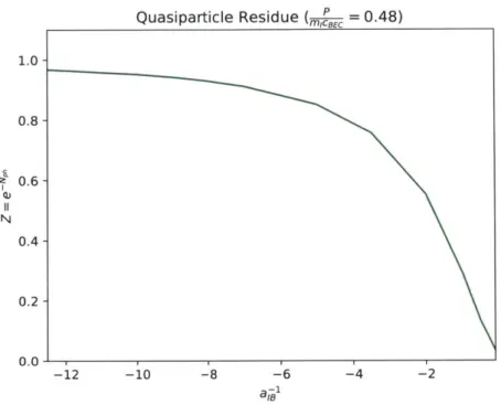
It is important to note that while the quasiparticle residue goes to zero in the Cherenkov phase regard-less of interaction strength, we can also get this quasiparticle breakdown in the polaronic phase at strong interactions (Fig. 3.5). Strong interactions also lead to sufficiently large numbers of phonon excitations to make the quasiparticle residue vanish. Therefore, at sufficiently strong interactions, the quasiparticle residue by itself cannot be used to distinguish between the polaronic phase and the Cherenkov phase.

-8 -12 -10 -2

renkov

=0)

Polaron

(Z>

0)

Quasiparticle Residue (mEcP = 0.48) 1.0- 0.8- 0.6-N 0.4- 0.2- 0.0--12 -10 -8 -6 -4 -2 a-1 aIB

Figure 3.5: Quasiparticle residue in subsonic region. The residue drops towards zero as we increase interaction strength.

4

Real-time Dynamics

We can now examine how the subsonic-supersonic transition in the ground state manifests in the quench dynamics of the system. Unless stated otherwise, the system parameters used were a mass ratio of I = 1 and a momentum cutoff A = 13.91[ -1] where is the healing length of the BEC.

In Fig. 4.1, we plot the Loschmidt echo and average impurity speed over time for various total momentum values. The total momentum value corresponds to initial momentum of the impurity as we are examining quench dynamics starting from a non-interacting impurity. Fig. 4.1(a) shows that the Loschmidt echo saturates to a finite value at long times for small momenta, but once we cross a critical momentum, we get a power-law decay to zero. This power-law decay in the dynamical overlap is resultant from a logarithmic divergence in the phonon number in the supersonic regime. Note that a true system would not produce infinite phonons as predicted by our calculations - this is an artifact of neglecting certain phonon-phonon correlations. However, the dramatic increase of phonons in the supersonic regime will still lead to the sharp decay of the Loschmidt Echo at the critical momentum. Nielsen et. al also predict this behavior in the supersonic regime [25], but find an exponential decay instead of a power law, a result of their Markovian master equation approach. Fig. 4.1(b) shows that the average impurity speed also has different behavior in the subsonic and supersonic regions; it saturates to some finite subsonic value when the impurity is subsonic but has a slow decay towards the speed of sound when we start the impurity supersonic.

We can examine these decays by fitting a power-law tail of the form t-^ to each curve. The exponents y of these fits for both the Loschmidt echo and the average impurity speed are shown in Fig. 4.2. Note that the exponents for both the Loschmidt echo and the impurity speed beccome nonzero at the same momentum; this indicates that the same critical momentum characterizes the behavior of both observables. This critical

momentum happens near -= CBEC for weak interactions but, at larger momenta as interactions get

stronger, the transition occurs at a larger momentum. We also see that the fit becomes noisy for stronger interactions (a-' = -2) and seemingly zero for a-' = -1.5. As we will see in the following plots, this is because the observables have already saturated to their final value; stronger interactions causes dynamics to converge more quickly.

(a) 100 6 x 101 4 x 10-1 3 x 10-10-1 100 101 10, t [1] (b) 3.0 -2.5 -2.0 -A Jed Q VEf 1.5- 1.0- 0.5-

0.0-Average Impurity Speed (a' = -5)

P MICBEC -- 0.10 -- 1.53 -- 0.52 -- 1.80 - 0.80 - 3.00 - 0.98 CBEC -- 1.28 0 10 20

Figure 4.1: Observables. (a) Loschmidt echo. at long times. Curves in the Cherenkov region impurity momentum. Curves from the subsonic Curves in the Cherenkov region all approach the

30 40 50 60 70 80

t [1]

Curves from the subsonic region saturate to a finite value decay to zero as a power-law at long times. (b) Average region saturate to different subsonic values at long times. speed of sound at long times.

Loschmidt Echo (a-'= -5)

P MICBEC - 0.10 - 1.28 - 0.52 - 1.53 - 0.80 - 1.80 - 0.98 - 3.00

0.5 -0.4 - 0.3-0.2 - 0.1-0.0 -0 2 8

Figure 4.2: Exponents characterizing long-time behavior observables. The power-law decay only starts after a critical momentum which depends on interaction strength.

1.2-1.0 -0.8 -A 0.4 -0.2 -

0.0-Average Impurity Speed

'Ur

.. . . !I, If a1 I',' / -- -10.0 . -5.0 - 0.5 2.0 --- -2.0 - 1.0 - 5.0 -1.5 -- < v,(t.)> =CBEC 0 2 4 <v1(t0)> CEEC 6 8

Figure 4.3: Final impurity speed. For weak interactions, the impurity ends up at the speed of sound if we start it supersonic. For strong interactions, the impurity will always end up subsonic regardless of its initial velocity.

Long Time Power-Law Behavior of Observables

Observable +++- -+++ - -5.0 . - -2.0 < . d -1.5 +~~-++ +-+-- 4-+_ + ++ -+- - - - M P m7rs-C-C

1.2 Loschmidt Echo 1 1.0- U.D Z-.- -5.0 -- 1.0 - 5.0 -2.0 - -1.5 0.8 - 0.4-0.2 -0.0 0 1 2 3 4 5 6 7 8 9 < vI(to) > CBEC

Figure 4.4: Final Loschmidt echo. For all interaction strengths, there is a range of initial impurity velocities where the the long-time dynamical overlap is nonzero followed by a range of initial impurity velocities where the long-time dynamical overlap is zero. The location of the discontinuous transition between these two regions depends on interaction strength and mass ratio.

(indexed by the total momentum of the system). In Fig. 4.4 we do the same for he Loschmidt echo. We determine the infinite time value of the observables by evaluating the power-law fit at long times. For cases in which the exponent of the fit is zero, this just results in an average of the last few values in the simulation (which is where the observable has saturated to). First, let us exaxmine the average impurity speed. For all interaction strengths, starting the impurity subsonic ((vi(to)) < 1) leaves the impurity subsonic at long times. The interaction strength in this subsonic case determines what finite subsonic value the impurity final reaches; we see the polaronic mass renormalization effect where stronger interactions and/or weaker masses lead to slower final impurities. For weak interactions, starting the impurity supersonic causes the impurity to end up at the speed of sound at long times; this is similar to the Cherenkov phase of the ground state. For intermediate interactions (e.g. a-' = -2), there is a region in which we start the impurity supersonic but end up subsonic. If we inject the impurity with even larger momentum, it will always end up at the speed of sound. For sufficiently strong interactions (e.g. a-' = -1.5), the impurity always ends up subsonic. An intuitive explanation for this behavior is that as interactions get stronger, the majority of the momentum that a supersonic impurity gives up is transferred on short time-scales. For very strong interactions, the impurity is very likely to have a large momentum scattering event and end up subsonic very quickly after which it stays subsonic. Weak interactions don't have a large enough matrix element to scatter into the subsonic region and so have a slower decay towards the speed of sound. If we turned on the interaction on more slowly instead of a quench protocol, we would probably end up with supersonic impurities traveling at the speed of sound even at strong interactions.

We can also examine the long time value of the Loschmidt echo as a function of the initial impurity speed. We see that the Loschmidt echo always saturates to a finite value for initially subsonic impurities, albeit to a smaller value for stronger interactions. For weak interactions, the value drops to zero as soon as the impurity is initially supersonic. For stronger interactions, we also get a sharp drop to zero after some critical velocity deep into the supersonic region. In cases where we expect larger mass enhancment of the subsonic impurity, the transition occurs at larger initial impurity speeds. Overall, the quench dynamics at long-times

does not exactly follow the ground state behavior though echos of the polaronic phase and Cherenkov phase still manifest. It is important to note that the discrepency between long-time quench dynamics and the ground state is noticeable primarily at strong interactions which is to be expected; the lowest energy state of the system is one where the impurity is traveling at the speed of sound along with a large number of lower energy phonons, but the quench dynamics at strong interactions gets stuck in a sector of Hilbert space with some larger energy phonons.

(a)(b _{Average Impurity Velocity (F=0.21} [ ]) Polaron Mass Enhancement (Subsonic Case)

T X Force Protocol (Harmonic BEC Trap)

0.5- 17.5- 0 Force Protocol (Homogenous BEC)

E Analytical Steady State 15.0- 0.4-12.5 El A 0.3 -V 10.0 -0.2- 7.5-0.1 5.0- 2.5- 0.0-0.0 0.0 0.5 1.0 1.5 2 0 2.5 3.0 3.5 4.0 -5 -4 -3 -2 -1 0 t [?I a

Figure 5.1: Effective mass protocol fully in subsonic region. (a) Average impurity speed. The impurity velocity increases linearly while the constant external force is applied. (b) Mass enhancement. We 'measure' a larger effective mass as we increase interaction strength.

5

Experimental Connection

We now connect our treatment of the Bose polaron system to experiment by suggesting a dynamical protocol to measure the effective mass of a polaron. We also show that this protocol is sensitive to whether the impurity is supersonic or not. While the sensitivity in this case is undesirable, it suggests a way to experimentally examine the Cherenkov physics of impurities in BECs.

The protocol is as follows. We wish to impart a known amount of momentum to the impurity using an external force and then measure the final speed of the impurity to determine the effective mass it felt. First, we start the system in a polaron ground state and then apply a constant external force to the impurity. We keep the magnitude of the force and the impurity's initial momentum fixed while only varying how long we apply the force. The inclusion of external forces and trap potentials to the equations of motion is done using a local density approximation (see Appendix A). The system parameters used were a mass ratio of " = 1.7, a momentum cutoff A = 36.60[ -'] where is the healing length of the BEC, an initial polaron state with total momentum Po = 0.15[mIcBEC], and an impurity-boson scattering length of aIB= -0.3[].

If we apply the force for a short enough time to keep the impurity in the subsonic regime, the impurity velocity saturates to a constant value (Fig. 5.1(a)). We can determine the effective mass of the polaron by reading off the final velocity of the impurity and dividing the known momentum imparted to the system by this velocity (Fig. 5.1(b)). As a check, we can compare the 'measured' effective mass in our simulation with that calculated using the saddle point solution to the equations of motion (Eq. 65). We see that the measured effective mass matches the saddle point calculation fairly well, especially at weak interactions.

If, however, we repeat this protocl after applying the force long enough to speed the impurity up into the supersonic regime, we get different results. We see dissipation represented by a curvature in the velocity as soon as we cross the speed of sound (Fig. 5.2(a)) which leads to the measured effective mass values drifting from the values determined from the saddle point calculation (Fig. 5.2(b)). The error with the saddle point calculation is equivalent at strong interactions in both plots cases because the effective mass has increased and the impurity is not actually supersonic in either case. We therefore see that Cherenkov physics rears its head and disrupts the effective mass protocol if the experimental setup is not sufficiently cold and/or the force is applied for long enough that the impurity becomes supersonic. This suggests, however, that we can use dynamics to probe the physics of supersonic impurities in a bath. Instead of trying to extract a dissipation constant from the experimental protocol described above, an experiment examining an externally-induced relative oscillation between the BEC and impurity would be better suited to probe this physics.

(b)