Design of linear hydrostatic bearings

Design of

Linear Hydrostatic Bearings

Christoph BrUnner

Submitted to the Department of Mechanical Engineering in Partial Fulfillment of the Requirements for the Degree of

Master of Science

at the

Massachusetts Institute of Technology

December 1993

j

Department of Mechanical Engineering December 17, 1993

Certified by /

Professor Alexander H. Slocum Thesis Supervisor

Accepted by

,., A;7

\

e: -

]Eng

\

ASS= 1ST U F

Professor Ain A. Sonin Chairman, Graduate Committee I .· x

1w

Design of Linear Hydrostatic Bearings

Christoph BrUnner

Submitted to the Department of Mechanical Engineering

in Partial Fulfillment of the Requirements for the Degree of Master of Science

Abstract

New materials and the ever increasing demand for higher precision place new demands in machine tool technology. New concepts are required with much greater dimensional and thermal stability as well as improved reliability and life span. Bearing technology is a criti-cal factor in machine tools, since they determine the machine's performance to a large ex-tent. One possible solution in bearing technology is the use of hydrostatic bearings. They provide the necessary high damping and stiffness as well as the robustness against

contam-ination with submicron dust particles generated during processes.

This thesis analyses and compares different kind of hydrostatic bearings for linear mo-tion applicamo-tions distinguished by the kind of flow restrictor used. Self-compensated bear-ings are discussed in detail and a new type of hydrostatic bearing, called HydroguideT M is presented that overcomes the disadvantages normally associated with this type of bearing. It reduces the influence of manufacturing errors on stiffness and load capacity, has no need for hand-tuning and has no small diameter passages and therefore does not clog. The bear-ing uses water as workbear-ing fluid, which allows for higher performance, and is environmen-tally friendly. The bearings thermal performance is improved by reducing the necessary pump power, and a greater heat capacity of water compared with normally used low-vis-cosity oil.

The fluid mechanics theory governing hydrostatic bearings is explained and formulas for the performance measures are derived. Since the HydroguideT M _{is deterministic the}

per-formance can accurately be predicted using a spreadsheet. Analytical studies are performed showing the influence of different design parameters. Based on these studies design rules for different applications are determined.

The advantages of this type of hydrostatic bearing are shown in two prototypes. Exper-iments were conducted verifying the theory. The results present performance measures, in-troducing capabilities and limitations of the bearing.

Thesis Supervisor: Dr. Alexander Slocum

Konstruktion Hydrostatischer Linearfuhrungen

Christoph Briinner

Abstract

Neue Materialien und die immer steigende Nachfrage nach Prizision erfordert neue Werkzeugmaschinentechnologien. Neue Konzepte mit hiherer dimensionaler und thermis-cher Stabiltiit sind erforderlich bei gleichzeitig verbesserter Zuverlissigkeit und erh6hter Lebensdauer. Fiihrungselemente sind ein kritisches Element im Werkzeugmaschinenbau, da sie zu einem groBen Teil die Genauigkeit der Maschine bestimmen. Eine m6gliche Li-sung in der Fihrungstechnik ist die Anwendung von hydrostatischen Lagern. Sie verfUgen sowohl iiber hervoragende Dimpfungseigenschaften, und haben eine hohe Steifigkeit als auch die notwendige Robustheit gegen Verschmutzung mit Staubteilchen kleiner als ein Mikron, die wahrend der Bearbeitungsprozesse entstehen.

Diese Arbeit analysiert unterschiedliche Arten hydostatischer LinearfUhrungen unter-schieden nach der Art des Vorwiderstandes. Hydrostatische Lager mit Laufspaltdrossel werden im Detail behandelt und ein neues Lager, HydroguideM, vorgestellt das die nor-malerweise mit dieser Art der Lagerung verbundenen Nachteile veringert. Es vermindert den EinfluB von Fertigungsungenauigkeiten auf die Steifigkeit und Nachgibigkeit, benitigt keine Nacharbeit und Feineinstellung der Vorwiderstiande und die Verstopfungsgefahr ist gering da keine Zulaufbohrungen mit kleinen Durmesser benitigt werden. Die Verwendung von Wasser als Schmiermittel ermiglicht eine hihere Leistung und macht das Lage umweltfeundlich. Die thermische Leistung des Lagers wird verbessert durch eine ver-ringerte notwendige Pumpenleisung und die hhere Wairmekapazitit von Wasser im Vergleich zu den normalerweise verwendeten Olen.

Die StiSmungsmechaniktheorie die das Verhalten des Lagers beschreibt ist erklirt und das Lager beschreibende Formeln abgeleitet. Da das HydroguideTM Lager deterministisch ist die kann die Leistung, mit Hilfe von einfachen Computerprogrammen prizise vorausge-sagt werden. Die Ergbnisse wurden in ein Tabelenkalkulationsprogram implementiert. Ana-lytische Studien wurden durchgefiihrt, die den Einflu3 verschiedener Konstruktionspa-rameter verdeutlichen. Aufbauend auf den Studien wurden Konstruktionsregeln fr ver-schiedene Anwendungsfalle aufgestellt.

Die Voteile dieses Lagers wird in zwei HydroguideT M _{Prototypen aufgezeigt.}

Acknowledgments

I would like to thank Professor Alexander Slocum. For all the inspiration and all things I learned during my studies at MIT.

Contents List of Figures 1. Introduction 10 1.1 Background 10 1.2 Statement of Objective 11 1.3 Thesis Layout 11

2. Theory on Hydrostatic Bearings 12

2.1 Operating Principle 12

3. Analysis of Linear Hydrostatic Bearings 14

3.1 Static and Dynamic Behavior 18

3.1.1 Fluid Mechanic Theory 18

3.1.2 Resistances 23

3.1.3 Effective Bearing Pad Area 26

3.1.4 Fluid Flow Rates and Fluid Velocities 27

3.1.5 Load capacity 27

3.1.6 Stiffness 28

3.1.7 Damping 28

3.2 Thermal Behavior 29

3.3 Design of Flow Restrictors 32

3.3.1 Constant flow devices 32

3.3.2 Laminar flow devices with fixed compensation 32

3.3.3 Laminar flow devices with variable compensation 33

3.3.4 Laminar flow devices with self-compensation 33

4. Comparison of Self- and Fixed-Compensated Hydrostatic Bearings 39

4.1 Load Capacity and Stiffness 39

4.2 Manufacturing Error 42

4.3 System Design 44

5 Case Study 1: Low Pressure Bearing 48

5.1 Design Considerations 48

5.2 Manufacturing 50

5.3 Bearing Design 51

5.4 Measurements 53

5.3.1 Straightness 53

6. Case Study 2: High Pressure Bearing 62 6.1 Design Considerations 62 6.2 Manufacturing 64 6.3 Bearing design 64 7. Conclusion 68 8. References 69 9. Appendices

9.1 Appendix A: Spreadsheet for Case Study 2 70

9.2 Appendix B: Mechanical Drawings for Case Study 2 75

9.3 Appendix C: Spreadsheet for Case Study 2 78

List of Figures

Figure 3.1: Stiffness and damping of a machine tool carriage. Figure 3.2: Bearing model and electrical circuit analogy. Figure 3.3: Fluid velocity profiles in hydrostatic bearing gaps. Figure 3.4: Fluid velocity profiles in hydrostatic bearing gaps. Figure 3.5: Fluid velocity profiles in hydrostatic bearing gaps. Figure 3.6: Bearing pocket geometry.

Figure 3.7: Squeeze film between two parallel plates.

Figure 3.8: Total power and power factor K for changing nominal gap. Figure 3.9: Flat-edge-pin: Laminar flow devices with fixed compensation. Figure 3.10: Variable compensation device (Diaphragm-Type).

Figure 3.11: Bearing pad and restrictor pad geometry.

Figure 3.12: The principle of self-Compensation using HydroguideTM. Figure 3.13: Load capacity of a self-compensated hydrostatic bearing. Figure 3.14: Stiffness of a self-compensated hydrostatic bearing. Figure 4.1: Load capacity of a fixed-compensated hydrostatic bearing.

Figure 4.2: Load capacity of a self-compensated hydrostatic bearing (Hydroguidem). Figure 4.3: Stiffness of a fixed-compensated hydrostatic bearing.

Figure 4.4: Stiffness of a self-compensated hydrostatic bearing (Hydroguidem). Figure 4.5: Manufacturing error of a fixed-compensated hydrostatic bearing. Figure 4.6: Manufacturing error of a self-compensated hydrostatic bearing. Figure. 5.1: Schematic of the hydrostatic bearing design using bearing blocks. Figure. 5.2: Low pressure hydrostatic test bearing.

Figure. 5.3: Bending moment on bearing blocks.

Figure. 5.4: Load capacity of the low pressure test bearing. Figure. 5.5: Stiffness of the low pressure test bearing. Figure. 5.6: Noise floor of the laser measurement system.

Figure. 5.7: Error motion of the carriage with 20 psi supply y pressure. Figure. 5.8: Straightness (250 mm) plot of granite bearing.

Figure. 5.9: The spectral components of the carriage's straightness error. Figure. 5.10: Straightness (100 mm) plot of granite bearing.

Figure 5.11: Noise level during straightness measurement.

Figure 5.12: Bearing pocket pressure as a function of supply pressure. Figure 5.13: Bearing pocket pressure as a function of supply pressure.

Figure 5.14: Figure 6.1: Figure 6.2: Figure 6.3: Figure 6.4: Figure 6.5: Figure 6.6: Figure 7. 1:

Dynamic response of the carriage with supply pressure on and off. Bearing arrangement (wrap-around) of case study 2.

Ceramic test bearing.

Load capacity of the high pressure bearing. Stiffness of the high pressure bearing.

Total power as a function of supply pressure.

Stiffness at zero displacement as a function of supply pressure. Properties of a self-compensated bearing.

Effective bearing area Specific heat capacity Load Capacity nominal bearing gap Stiffness

Friction power Pump power Pressure

Supply pressure

Pressure difference between upper and lower bearing pad

Fluid flow Resistance

Resistance of upper restrictor pad Resistance of lower restrictor pad Resistance of upper bearing pad Resistance of lower bearing pad Fluid velocity Restrictor resistance Dynamic viscosity Kinematik viscosity Density Displacement Fluid shear stress

to bearing resistance ratio

[Nsec/m2] [m2/sec] [kg/m3] [m, gm] [N/mm2] List of Variables Aeff: c F: h: K: Pf: Pp: P: Ps: Ap: [m2] [J/kg K] [N] [m, gm} [N/gm] [WI [W] [Pa=N/m2] [Pa=N/m2] [Pa=N/m2] [1/min] [Nsec/m5] [Nsec/m5] [Nsec/m5] [Nsec/m5] [Nsec/m5] [m/sec] Q. R: Rur: Rlr: Rub: Rib: v: :. Al: V.

p:

6:

1. Introduction

Linear and angular bearing technology is a critical factor in machine tools, since they determine the machine's performance to a large extent. They have to guide the relative moving workpiece and tool with a high degree of accuracy repeatable over time. To mini-mize the error motions introduced by bearings they must provide superior performance in terms of stiffness, load capacity and damping as well as motion resolution. In addition, bearings contribute considerably to the machine's manufacturing cost.

In most machine tool applications rolling element or hydrodynamic bearings are used. Hydrostatic bearings provide the superior performance characteristics that are desired, but are not widely used because of several disadvantages generally associated with this type of bearing. They require expensive support equipment, such as pumps, filters, and collection systems and are therefore expensive. Furthermore they need careful monitoring and main-tenance for reliable operation. The design relies mostly on experience, since their perfor-mance can not be predicted accurately and for that reason a considerable amount of hand-tuning is necessary during assembly.

However, a new type of hydrostatic bearing was developed that overcomes most of these disadvantages. It requires lower flow rates, therefore smaller pumps and hence gen-erates less heat. It is less sensitive to manufacturing errors, requires no hand-tuning, uses water instead of oil as working fluid and is deterministic. The bearing's performance is described by simple equations and can be predicted accurately.

1.1 Background

New materials and the ever increasing demand for higher precision place new demands in machine tool technology. E.g. manufacturing ceramics economically with a high degree of accuracy is one of the challenges for future machine tool technology, since they require ma-chines with much greater dimensional and thermal stability. In addition, the durability of machines has to be improved. Since ceramic particles of submicron size are produced dur-ing the process that wear seals and ultimately damage slide-way and spindle beardur-ings, par-ticularly rolling element bearings.

One possible solution in bearing technology is the use of hydrostatic bearings. They provide the necessary high damping and stiffness as well as the robustness against

contam-ination with ceramic dust. The new self-compensated hydrostatic bearing presented fits these needs.

1.2 Statement of Objective

This thesis analyses and compares different kind of hydrostatic bearings distinguished by the kind of flow restrictor used. Self-compensated bearings are discussed and a new type of hydrostatic bearing, called HydroguideTM is presented that overcomes the disadvantages normally associated with this type of bearing. Design rules are derived and solutions are introduce that show the implementation of the theory. Performance measures are provided, that show the capabilities and limitations of the bearing. This thesis can be used as a guideline comparing the HydroguideT M _{to other bearings and to guide a design of a linear}

motion system using HydroguideTM.

1.3 Thesis Layout

The second chapter illustrates the theory on hydrostatic bearings and explains the operating principle. Since hydrostatic bearings are distinguished by the kind of flow restrictor used, different restrictors are introduced and their advantages and disadvantages are discussed briefly. Chapter 3 derives the basic equations, that describe the mechanical and thermal behavior of hydrostatic bearings. Formulas for the most important performance measures, for instance load capacity and stiffness, are derived and implemented into a spreadsheet.

In chapter 4 different kind of flow restrictors and a new type of hydrostatic bearing called HydroguideTM are introduced. Using the spreadsheet written, parameter studies show the performance of bearings with different restriction under varying conditions. Fixed compensated and self-compensated bearings using HydroguideTM are compared in detail. Chapter 5 and 6 describe the application of the HydoguideTM to linear motions, pre-senting two prototypes build during the course of this thesis. Design and testing are dis-cussed in detail.

2. Theory on Hydrostatic Bearings

2.1 Operating Principle

Hydrostatic bearings utilize a thin film of externally pressurized fluid between the relative moving parts to support loads. The fluid is supplied with high pressure to bearing pockets from which it flows across lands restricted on the opposite side by the bearing rail. The distance between bearing land and rail is generally referred to as bearing gap. This gap restricts the flow out of the pocket, leading to a difference between the pocket and the am-bient pressure. This differential pressure times the land area is the force that supports the load. Since pressure is distributed over a large area of several bearing pads, large loads can be supported. In order to obtain bidirectional stiffness and load capacity, the support bear-ing can be preloaded by means of an opposed pad, the preload bearbear-ing pad. Since this is most common in machine tool applications, this configuration will be discussed in this thesis.

As the bearing is loaded it is displaced and the load bearing gap decreases, while the preload bearing gap increases. Positive displacement S is defined as decrease of the load bearing gap as response to a positive load. In order to realize different equilibrium positions at varying loads differential pocket pressures must be realized. This is possible by regulating the inlet-flow into the bearing pockets. Flow restrictors in series with the bearing pockets serve this purpose which is generally referred to as compensation. Without compensation the bearing would not be able to support any load. Different restrictors and advantages are discussed. With varying loads applied, the bearing displaces according to its stiffness and load capacity. Stiffness and load capacity are itself a function of the bearing gap. The influence of bearing displacement will be discussed in chapter 3.

As the bearing moves along a rail the straightness is determined by the pressure fluc-tuations in the supply lines, the heat generated into the system, the first order straightness of the rail and the tendency to build up a hydrodynamic wedge at higher speeds. Since the load is distributed over the bearing area, parallel and straightness errors smaller than 1/10 the bearing gap will not result in an error motion of the supported carriage.

There is very low friction in hydrostatic bearings in particular no static friction at all. At low speeds it operates without stick slip effects. The motion resolution therefore depends only on type actuators and, sensors and controllers and there will be no positioning error

introduced by the bearing using an indirect measurement system. In addition, there is no wear and if properly handled hydrostatic bearings have potentially infinite life.

Power is generated by two sources during operation and entirely dissipated as heat: The pump power and viscous shear power in the fluid introduced by the relative moving parts. The former dominates in linear motion systems, due to generally low speeds (vmax ca. 30m/min for a surface grinding table). The pump power is the product of pressure and flow. Assuming a fixed pressure for a desired load capacity, reducing the flow is the best mean of reducing the power introduced into the system.

Hydrostatic bearings normally use oil as working fluid (e.g. ISO 10 oil with [l=0.01 Nsec/m2). Oil has desired properties, it is an excellent lubricant and long term stable, but its viscosity is high and its heat capacity is low. High load capacity and stiffness require small bearing gaps. With smaller bearing gaps the resistance increases and lower viscosity fluid are desirable to reduce the vicious shear generated due to the high resistance. Water has one tenth of the viscosity of low viscosity oil and four times the heat capacity. Water decreases the power generated and transferred into the system, provides higher performance and is environmentally friendly.

3. Analysis of Linear Hydrostatic Bearings

The force exerted on the fluid film against the rail and the carriage must, by equilibrium, balance the applied bearing load. The response of the machine to these forces depends on its stiffness, damping and its mass. Stiffness and damping are each necessary, but individually not sufficient for a precision machine. Damping in hydrostatic bearings depends on the velocity of the carriage with respect to the base. Thus, the bearing may not be much stiffer than the machine structure, because very little damping in the bearing would occur. Bearings are critical elements in the structural loop of the machine, since their static and dynamic behavior has a significant influence on the overall response.

In a machine tool as shown in Figure 3.1 the importance of bearing technology to the overall performance and the influence of stiffness k and damping factor c of a linear guide can also be interpreted in terms of workpiece accuracy. As the static force displaces the carriage with respect to the tool errors are introduced, which result in shape inaccuracy. Damping dissipates the energy generated by vibrations. The less damping is provided and therefore the less energy is dissipated by the bearing the larger are the responding error motions of the carriage with respect to the structure. The damping factor determines the surface finish of the workpiece to a large extent. Hydrostatic bearings comply with these high demands and there performance can be analyzed and predicted using a simple fluid model

Figure 3.1: Stiffness and damping of a machine tool carriage.

In order to support bidirectional load most applications of hydrostatic bearings are preloaded by means of an opposed pad configuration. This configuration is analyzed using the law of Hagen-Pousseuille P=QR, in analogy to the law of Ohm for electrical circuits. A

pressure source and four restrictors are used to model the hydrostatic bearing. RI and Rp are the load and preload bearing pad resistances, while the resistances at the entrance to the bearings provide a means of regulating the flow and therefore establishing a differential pressure between the upper and the lower bearing pad. These are generally referred to as restrictor resistances or compensation. Figure 3.2 shows the bearing model and the electrical circuit analogy for the opposed pad hydrostatic bearing.

Rload

\MMA/-MM

,\M/V'\

'M4Mt

p

J

Figure 3.2: Bearing model and electrical circuit analogy.

Using this model the nominal total fluid flow resistance of the undisplaced opposed pad hydrostatic bearing, modeled from two resistances in parallel each consisting of two resistances in series, is

R

I

(3.1)

R+R, R+Rp

This leads to the pocket pressure and the pressure difference in the load and preload bearing pad. The pocket pressure in the load bearing is

Pi Ps R+R

)

(3.2)

The pocket pressure in the preload bearing is

I I

1

PP =(S Rp (3.3)

The pressure difference is thus

~Ap= PI - pp F tR.I_ R P ) (3.4)

AP=PI~PP=PslRR=

R+Rp

As seen in equation (3.4) for zero as well as infinite restrictor resistances the bearing is not able to support a load since the differential pressure between the opposed bearing pad equals zero. The ideal resistance for maximized differential pressure is found by taking the partial derivative of the pressure difference with respect to the restrictor resistance. Assuming that 6<<h we can neglect all non linear 3-terms the ideal restrictor resistance for the fluid circuit that balances the resistance bridge is

Rideal= _ with = Rrestrictor (35)

h3 ' _gRbearing

Thus, the pocket pressure for a changing bearing gap, i.e. under displacement can be determined. The pressure in the load bearing pocket under displacement is

Pi = Ps(_)3

h

and the pressure in the preload bearing pocket is

Pp

=PS(h+ 6)

The pressure difference between the load and preload bearing pad in an opposed bearing configuration under a displacement 6 is thus

1 1 (3.8)

AP = P - Pp =Ps((h

-

)3h

(h

+)3+h3

(3.8)

Again, it is obvious that at zero displacement both pocket pressure are equal and the resulting pressure difference is zero.

3.1 Static and Dynamic Behavior

The static and dynamic behavior of hydrostatic bearings is determined by the properties of the fluid film. As shown in the following chapter, the pressure distribution in the bearing pads can be analytically determined. The load that can be supported by the bearing is therefore the sum of the products of pressure times the area of several elements of the bearing geometry. A typical geometry of a hydrostatic bearing pad is shown in Figure 3.6 For the analysis the bearing is devided into regions analyzed by using different forms of the Navier-Stokes equation.

As seen earlier, it is possible to model fluid systems in analogy to electric circuit systems. In the same way the law of Hagen-Pousseuille corresponds to the law of Ohm, the rules for electrical resistances in parallel and series apply for fluid resistances. To be able to model the entire bearing system the resistances have to be determined first.

3.1.1 Fluid Mechanic Theory

The knowledge of pressure distribution in the bearing pocket is essential for the derivation of equations describing the behavior of hydrostatic bearings. Assuming a laminar, viscous flow between two parallel plates the Navier-Stokes equation is applied describing the motion of the fluid [12]. This differential equation of motion of a viscous fluid is very difficult to apply, but analytical solutions can be obtain for a few simple flows. Fortu-nately, the flow in the bearing pads can be modeled obtaining a simple solutions. Consider-ing steady flow with a velocity field dependConsider-ing only on two spatial dimensions and choos-ing appropriately simple boundary conditions.

To describe the flow in different bearing geometries it is necessary to express solution in the cartesian as well as the polar form of the Navier-Stokes equation for an incompress-ible fluid with constant viscosity. The general form of the Navier-Stokes equation is

DV = _Vp + g + VV2V (3.9)

Dt

p

with (1/p)Vp , g, VV2V the pressure force, the gravity force and the viscous force

for the cartesian form demonstrating the underlying fluid mechanics. The same principle applies for the polar form for which solutions are derived as well.

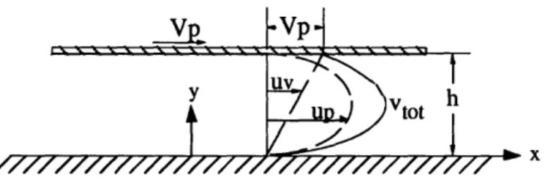
In the case of hydrostatic bearings, fluid flows through narrow channels by means of a pressure difference and an additional velocity component introduced by the carriage moving at a constant speed V. For both cases the fluid profile, the flow rate and the resulting pres-sure distribution can be determined separately. The flows are generally referred to as 'Plane Couette Flow' and 'Plane Poiseuille Flow' respectively.

In the case of 'Plane Poiseuille Flow' the flow is restricted by two fixed parallel plates separated by a distance h, the bearing gap. For hydrostatic bearings this corresponds to a carriage sitting stationary. The following assumptions can be made: the pressure gradient is constant in x-direction, a positive fluid velocity V in the x-direction as a function of y, and all remaining velocity components zero. Thus, substituting these assumptions the cartesian Navier-Stokes equation is reduced to

0= ldp d 2u (3.10)

p=

Note that u and p depend only upon y and x respectively, and thus by integrating twice and applying the boundary conditions of zero velocity on the walls, u(0)=0 and u(h)=0, the constants of integration can be determined and the velocity profile u(y) is found

U = I p (y2 - yh) (3.11)

2pv dx

Umax 8 , at y=h/2 (3.12)

This flow is parabolic with the maximum velocity (umax) at the center of the channel as shown in Figure 3.3.

Y

4

Figure 3.3: Fluid velocity profiles in hydrostatic bearing gaps.

The flow rate through a cross section of area dh, where d is the depth of the parallel plates, is found by integrating twice across h

Q = udA = - dx)ly(h- y)dydz (3.13)

Q (dp d ) 2 3 h (3.14)

dh3 _{(= dp) (3.15)}

Q

dx

Thus, we can determine the pressure distribution of the laminar, viscous flow in the gap due to a differential pressure. The x-dimension, in the case of the hydrostatic bearings, is called land width 1. Integration across 1 in x direction therefore yields

P2 -12#Q

J

dp=

~dh3

fJx

(3.16)

P

d-"-3-

(3.17)

Assuming, that the pressure pi is atmospheric pressure, Ap is the gage pressure along the bearing land width 1. In most applications the atmospheric pressure is assumed to be zero and the equation reduces to

P1 -= dh3 Q (3.19)

The same analysis applies to the polar form of the Navier-Stokes equation in order to determine the pressure distribution for rounded parts of the bearing pad. Again, assuming Plane Poiseuille Flow the polar Navier-Stokes equation reduces to

1 ap d2u

-idr =d 2 (3.20)

,#

r

=

_z

2

By integrating twice and applying the boundary conditions of zero velocity on the walls u(z=0)=O and u(z=h)=0, the constants of integration can be determined and the velocity profile is found

U = I d(Z2 ' -_zh) (3.21)

2 dr

The flow rate out of a full annulus is found

h

1

_AP

_j27rh

Q

o 2. at/0 o

Q=

r

r

₎

Thus, we can determine the pressure distribution by integration across 1 in r direction, with rp the inner radius and 1 the land width as shown in Figure 3.6.

P2 -6Q'r P+1dr

f dp2 - 6 r, fQ dr _(3.24)

Pi r

And the pressure for a full annulus distribution is found And the pressure for a full annulus distribution is found

Ap= (3.25)

Steady viscous Plane Couette Flow exists when one of the parallel plates moves at a constant speed Vp in x direction, that depends on y only. Since there is no pressure difference between the inlet and the outlet, there is no pressure change imposed on the flow. The velocity along a streamline is constant so that the material derivative DV/Dt equals zero. Noting that only y derivatives are non zero the Navier-Stokes equation reduces to

0= vdu

(3.26)

o~2u

d =u 0 (3.27)

dy2

Integrating twice and determining the constants of integration by applying the boundary conditions u(y=O)=O and u(y=h)=Vp yields the velocity profile as shown in Figure 3.4.

u=V p h (3.28)

P

~

~

hV

A

y

l

y

l

l1 ~ x

M-

Figure 3.4: Fluid velocity profiles in hydrostatic bearing gaps.

The flow rate in x-direction through a cross section of area bh, introduced by the moving plate is found by integrating twice across h

a=jld4dd d *VP (3.29)

Q = VdA = dfudy= Y (3.29)

h 2 0

Q = -dVph (3.30)

2

It should be noted, that for the calculation on hydrostatic bearings the later is of minor importance, because even in the case of a moving carriage when the pressure distribution changes the net pressure across the bearing pad basically remains unchanged. Therefore the basis of the bearing calculations is the pressure distribution due to Plane Poussieulle flow. But it is important to know the total fluid velocity and the total fluid flow rate in order to determine a condition for the maximum carriage velocity. As a general rule he flow rate due to the pressure difference should be on the order twice that due to the flow dragged into the bearing by relative motion. The maximum speed of the carriage supported by a bearing with y=1 and the smallest pocket pressure p is

ph2 Vmax 12

12/g,~

(3.31)

The Navier-Stokes equation for both flows is linear and thus the resulting flow can be attained by superposition. The combined fluid velocity profile due to a moving plate and a constant non zero pressure gradient is shown in Figure 3.5.

x

Figure 3.5: Fluid velocity profiles in hydrostatic bearing gaps.

3.1.2 Resistances

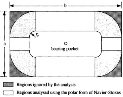
Applying the results from the fluid mechanics analysis the according to the law of Hagen-Poussieulle p=RQ the resistance for a single bearing pad can be calculated [1] [3]. Therefore the bearing pad is divided into several regions as shown in Figure 3.5 enabling a analysis using the two forms of the Navier-Stokes equation. The resistance Rs for the straight regions are taken together and described by a land width d containing all four regions. The resistance Rp for the four polar regions can be attained by deriving the solution for a complete annulus as derived before.

I b -I

a

·: Regions ignored by the analysis-..

[I I Regions analysed using the polar form of Navier-Stokes

.... Regions analysed using the catesian form of Navier-Stokes

Figure 3.6: Bearing pocket geometry.

The total resistance of the rectangular bearing pocket is thus

1 1

R =

+-

(3.32)

R RP

and with the distance d, the theoretical depth of the straight bearing regions

d =2(a+b+-4(l

+ rp))

(3.33)

the fluid resistance Rs becomes using the solution for plane Poussieulle flow as derived earlier

R',= 61y ~(3.34)---

-(a + b - 4(1

+ r))h3

Assuming a full circle annulus the resistance Rp of the rounded regions becomes

(rp +)

6R = log (3.35)

R.=

rh

(3.35)

With these two resistances the total resistance of a rectangular bearing pocket is

7

a+b-4(l +

r)

The actual flow resistance of the load bearing pad under a displacement is

(

=(h-8)

(h - .+

a+b-4(1+rp)

The actual flow resistance of the preload bearing pad under a displacement is

7

(h + )3

(h + i)3

a+b-4(1+rp)

i+ I

Assuming laminar, viscous flow the resistance of the bearing pockets is found to be a function of the pad geometry, the bearing gap and the viscosity of the fluid. Thus, as the bearing is loaded and displaced the bearing gap and therefore the bearing pads resistance changes.

(3.37)

3.1.3 Effective Bearing Pad Area

To determine the force exerted on the bearing pads the effective bearing pad area must be considered. The effective bearing pad area takes into account the pressure drop across the bearing lands.

The entire pocket area is

AP, =(a - 21)(b - 21)+ r(r- 4) (3.39)

The total land area over which viscous shear occurs in the bearing gap is

Al = ab - Ap (3.40)

For the straight land regions of Figure 3.5, the pressure decays linearly from the pocket pressure to zero, and the effective area of the straight lands is therefore half of their actual area

As =(a+b-4(+rp)) (3.41)

For the rounded regions of Figure 3.2, the pressure decays logarithmically from the pocket pressure to zero. The effective area therefore is

ArI 1(2r+) _2 (3.42)

f

This yields a total effective bearing area of

An~

=(- -4(a

21~-r

(3.43)

3.1.4 Fluid Flow Rates and Fluid Velocities

The total fluid flow rate for the undisplaced bearing at nominal bearing gap is

Q P = Psh3

R y (3.44)

The lowest flow velocity occurs at the outer circumferences of the bearing pad. It is the fluid flow rate out of the bearing pocket divided by the area the fluid flows through. The flow rate out of the upper bearing pad a at displacement 3 is

(3.45)

(3.46)

Qub = P

Rub

and the velocity of the fluid leaving the upper bearing land is

Vub

_{Vb 2(a + b)(h - )}

The flow rate out of the lower bearing pad a at displacement is

Q pib

Rib

and the velocity of the fluid leaving the upper bearing land is

(3.47)

Vib = Qlb (3.48)

2(a + b)(h + 3)

3.1.5 Load capacity

The Load capacity is load that the bearing system can support at a given displacement 3. It is the pressure difference of the opposed bearing pockets times the effective bearing area. Since it is a function of the supply pressure and the area of the bearing pads it can easily be increased by increasing the two variables.

[

1

1_

F = AffA = psAf h

_[3h]

_[(h+[-

_{; ;}

_(3.49)

3.1.6 Stiffness

Stiffness is the partial derivative of the load capacity with respect to the change in bearing gap, the displacement 6.

dF

K=

K=~

3Ph[(h

5)3

+ h3]

+

+

5)3+

3.1.7 Damping

Damping in hydrostatic bearings is achieved through the energy dissipated in the fluid film. This is generally referred to as squeeze film damping. As the fluid film is forced out of the bearing gap, due to viscous effects the fluid resists this extrusion and a pressure is build up. Thus the approach is slowed down. By the action of varying loads the fluid film is not only subjected by the squeezing action but also by the absorption in each cycle. Therefore, due to the large areas of fluid film hydrostatic bearings provide excellent damping.

force

. f w

Figure 3.7: Squeeze film between two parallel plates.

Analytical solution describing the damping capability of small fluid films can be obtained, but are only rough approximations and the assumption made are not always valid. Thus, results can differ significantly for different applications. However, a simple formula as derived by Fuller [8] is helpful in gaining a better insight to the effect of squeeze film

damping. The formula is derived for two parallel, rectangular plates of width w and length 1 assuming two dimensional flow. The damping factor is

l1W3

b = K hw3 (3.51)

where pu is the viscosity of the fluid and Ks a geometric factor related to the bearing. For /w > 10 Ks = 1.

As stated before, the larger the areas the larger the damping capability. The smaller the bearing gap and the larger the viscosity, the better the damping. It should be noted, that squeeze film damping does not depend on the pocket pressure. Thus, the damping capability is the same for all types hydrostatic bearings.

It should be noted that the area of hydrostatic bearings is restricted by the application and the choice of the fluids viscosity greatly influences the bearing gap chosen. Therefore a trade off between the desirable fluid qualities and the damping has to be found.

3.2 Thermal Behavior

Power is generated by two sources and entirely dissipated as heat. Pump power and friction power. Pump power is the energy that forces the fluid through the bearing. Friction power is the energy necessary to move the carriage. Both are dissipated due to viscous shear loses in the bearing. The calculation of power assumes laminar flow in all parts of the bearing the bearing pockets, the bearing lands and the fluid supply lines. The area where turbulence is most likely to occur are the bearing pockets. Thus, the condition for laminar flow in the bearing pocket is a Reynolds number

Re = vhpp (3.52)

smaller than 2000. Turbulent flow, i.e. large Reynolds numbers, increases the friction in the fluid and the shear stress on the walls significantly and therefore leads to a significant increase in temperature. The equation stated are not valid for this case.

The pump power is calculated as the product of total fluid flow and supply pressure. With the fluid flow Q as derived earlier the total pump power becomes

Pp = QP = _(3.53)

The friction power which must be transmitted through the moving surface is the product of the friction force and the surface speed. The equation for the shear stress according to Newtons law of viscosity of two plates moving relative to each other at a distance h

du v

= 7 -= (3.54)

dy h

and the force required to shear a surface of area A

F = At (3.55)

lead to the equation for the friction power

Pf =Ff V =vV2(A +4 Pocket (3.56)

It should be noted that the pocket area contributes to a larger extent to the friction losses than the land areas. The factor four accounts for these addition losses considering recirculating flow in the pocket. The total power generated in hydrostatic bearings is the sum of the pump and the friction power

Ptotal = Pp + Pf (3.57)

Another alternative form of this equation is

Ptotal = P, (1 + K), with K=Pf/Pp (3.58)

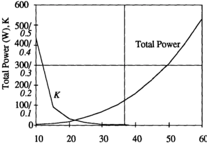
where K is the power ratio also indicating the proportion of hydrostatic to hydrodynamic effects. Pure hydrostatic load support leads to K=O, what in fact means zero velocity between the parts. According to this characteristic K can be used as a measure for distinguishing hydrostatic bearing in 'low speed' bearings with K<1 and 'high speed' bearings with K>1.

UnA

3o.

Figure 3.8: Total power and power factor K for changing nominal gap.

From Figure 3.8 shows the total power and the power ratio K for a linear hydrostatic bearing running with a velocity of 0.5 m/sec (30 m/min). A larger gap influences the total power significantly increasing the pump power exponentially. As the gap decreases the shear power gains relative to the pump power more importance, but due to low speeds never reaches a level dominating the total power. Since linear hydrostatic bearings seldom move faster than 0,5 m/sec they can generally be regarded as low speed bearings. For the bearing configuration simulated above, using water as fluid and a supply pressure of 10 atm, the total power at a 10lm gap is only 3.5 W.

The factor K indicates that the shear power never accounts for more then 50 % (i.e. at a 10 mg gap K= 0.425 and Pf-1.5W) of the total power. This is due to the decreasing flow rates of the bearing. At laminar speeds using water with its low viscosity ( =0.001 Nsec/m2) decreases the power generated by an order of magnitude compared with normally used oil (ISO 10 oil with u =0.01 Nsec/m2). In addition, the water has twice the heat capacity of oil. In order to achieve the same magnitude of total power for oil bearings the gap has to be expanded reducing stiffness and load capacity significantly.

The temperature rise in the fluid from the entry of the bearing to the end of the bearing can be calculated assuming that the energy is convected from the bearing.

AT = P.oa (3.59)

JcpQ

Most machines require that minimum heat is introduced into the machine. Thus, it is necessary to minimize the power for a given load capacity. Minimizing the total power is achieved by minimizing the fluid flow and increasing the heat capacity of the fluid. Small bearing gaps produce small flow rates, since the resistance of the bearing is inversely proportional to the cube of the bearing gap and hence lowering power generated. However the friction power increases with smaller gaps and can produce an significant amount of heat at higher speeds. Low speed bearings don not suffer from this particular problem especially when using a low viscosity fluid.

3.3 Design of Flow Restrictors

As it was shown, hydrostatic bearings need a flow restrictor in order to support varying loads. There are four different types of bearings, distinguished by the kind of flow restric-tor that regulates the inlet-flow into the bearing pocket. All provide the necessary pressure difference to support varying loads. However, the design of flow restrictors is critical, since it determines the overall performance of the bearing and the cost to a large extent. This thesis is concerned with the design of bearings using self-compensation, the other compensation methods are described only briefly.

3.3.1 Constant flow devices:

To provide constant flow to the bearing pockets, regardless of the bearing gap displacement is achieved by several methods. One uses one pump per bearing pad, but since this method is expensive more often a single pump and flow dividers are used to distribute the flow equally to the bearing pockets.

This methods provides the largest stiffness, but is expensive and due to the tendency of normally used oil to change the viscosity with changing temperature the undesired amounts of fluid flow can degrade the performance of the bearing or in the extreme the bearing is not able to support any load at all.

3.3.2 Laminar flow devices with fixed compensation:

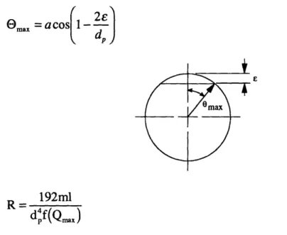
There are several restrictor providing a fixed restrictor resistance regardless of the operating conditions, i.e. changing bearing gap. Most of them make use of the fluid resistance of small diameter passages. Flat edge pins, when pressed in a hole provide simple means of creating a resistance. As also do capillary tubes of small inner diameter. In order to achieve the desired resistances the diameter have to be on the order of 0.4 mm.

Omx =aco dp J

E

192ml

R=

dpf(Qmax )

Figure 3.9: Flat-edge-pin: Laminar flow devices with fixed compensation

There are several disadvantages associated with fixed compensated hydrostatic bearings. Load capacity and stiffness are half of self-compensating bearings and the flow in the restrictors tends to turn turbulent and therefore generates undesired heat and mechanical noise. The small diameter passages tend to clog and due to the sensitivity to manufacturing errors both compensation devices must be expensively hand-tuned during assembly in order to match the bearing pad resistance and to optimize performance.

3.3.3 Laminar flow devices with variable compensation

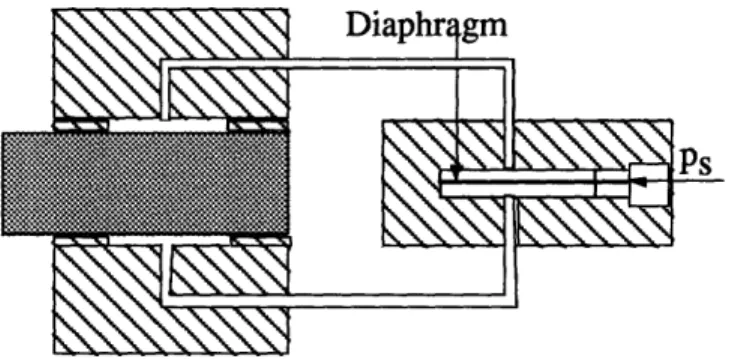
Laminar flow devices with variable compensation, as the type shown in Figure 3.10 include the use of diaphragms or valves to provide a flow inversely proportional to the pocket resistance. Thus, they create a larger differential pressure then created with the use

of fixed compensation devices. Even they achieve higher performance then fixed compensated bearings, they suffer from all other disadvantages described for fixed compensated bearings.

Figure 3.10: Variable compensation device (Diaphragm-Type)

3.3.4 Laminar flow devices with self-compensation:

Self-compensation, according to the principle of self-help [5], is based on the principle that high pressure fluid can be regulated through passages on the bearing surface. The restrictor resistance is achieved by the same means as the bearing pad resistance. The fluid than flows to the opposed bearing pocket. All self-compensated bearing designs follow this principle. There are a variety of self-compensated bearing designs, first developed during the 1940's. They all suffer from detrimental fluid flows, which decreases the performance. In addition due to the complex fluid pattern, they are not deterministic and their performance is difficult to predict. But these effects can be eliminated by proper design of the compensation devices. A new design, called HydroguideT Mis described in detail.

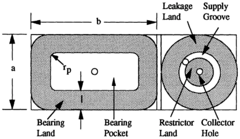
As shown in Figure 3.11 and 3.12 the fluid flows out of the pocket on the surface of the bearing, across restrictor lands, whose area is tuned to that of the opposed pocket's land. It then flows into the small collection pocket that is connected to a large bearing pocket on the opposite side of the bearing rail. The resistance of the compensator, and therefore the flow is now controlled by the change in bearing gap. The compensation device and the corresponding bearing pocket experience the same magnitude of displacement, but with different signs. When a positive load is applied the load bearing's gap decreases resulting in increasing flow resistance. The corresponding compensator gap increases, decreasing the flow resistance, and thus providing a larger flow to the bearing pad that is resisting the load.

L

b

-|

1

·x·: ::;····-·

...-..-.`:....':;.;;S·:-':St;::::: _s.·.·. ,··:r.:·:·:·:·:·:·:.::I:: j_{::':::::'i:·::·:·:·.·t.. ;·.··I····} 5:::::.:::;:;5::::i:::i:S$iiiiiiijiiji.i·;;.:·.: _{X· i*::} : _{.;·.5·;·;·5·i}r····

;.S'.'f;:5· ·ir5·-·

:: ,,,, g185881

5x·: :s·.;·:

:'· 8 i:i::j: _''2 ,:,zyj:n_{r.·.·.··;.s·.·.·.;·.} :::::::::.:::::: _ui:$r::: f _·-·,·· i8#8i ::;:··I 8P:·:j P O ::r.: _{:8R:i :x;} iSIiiii ;·:;:;: _{.·.r·.·.·.·.} i::x: _{·.· .··.·.· )j:} · _jj! "'.""" .;···rr _{· · ·· I··} sr .

:'"::::::::i _·: "xi::8: .:'.'Y ·rS·'_{I:':':::j .·.·.·.·.s·.·}

· :Y:c:: :·::::::::::::::::::·5:·:·:·:·:·:·:·:·:· :.:.::::::::::::::: :'';:···1'';.:::::.::5j:·:.: _:::::: · · · ·:····i::::2i·:::1::·::::. _{·.·.·. ·;.·;·.·.;} ::::::::·j::::::::::: ::····:·:; _{· ·· · ·.::: ·. :::::Y::::::::::i} ·· ··· ·· ::::::! _'" · · ·· ·· · ·· ·· ·_s·.·.·. · · · :··:·:···8#::#8#::r:.x· ::::·:·::·::::::·::::: ::·:·::::·:j·:::::·:·:'::b::.;L..;. 3 .::::::::·:·:·:.:.:·:::::·::i''''';'5 1 ·'·:·:·:·:·'·'·:·:·:·:·:·:·:- ::...:::::::'.·::.1·:·:··:5 rr;s;;.; ':::;:;:;:;:::,;::;:;·;1 i :·,. _{;;;Si·;.;;s..r;r;.;;1··;···;·1··1··} :::.liZ:::::::1:::iisi:::: ...,.,....;..:,,._{··;;·;·· ·0:·:::·:·:;:·:·:·:·:5.:·:·:·:·:;:':·:·5'' L····5··} t

--

Figure 3.11: Bearing pad and restrictor pad geometry

A new design is proposed, called HydoguideTM_{. It overcomes the disadvantages}

generally associated with hydrostatic bearings. The Hydroguide TM _{has a compensator} geometry leading to flow pattern accurately known in advance. The flow restrictor consist of round and linear lands with the least complex shape. The least complex shape, not incorporating linear lands is a complete annulus as shown in Figure 3.11. The flow pattern is constant and easy to analyze. The results of the analysis can be easily incorporated into spreadsheets accurately predicting the performance of different bearing configurations.

Compensation

Flu

>*L~ Z

Since it has no small diameter passages (the smallest diameter hole is 3-5 mm) the bearing does not tend to clog. Even in case of contamination, small parts supplied with the fluid to the compensator will be ground away in the bearing gap through the moving carriage. Thus the bearing is entirely self-cleaning.

The effect of self-cleaning and the insensitivity to contamination allows the use of water as bearing fluid instead of normally used oil. Water has the inherent property to self-contaminate through biological effects and is not suitable for other bearing designs. It has a high heat capacity and excellent thermal conductivity. This reduces the heat generated by the bearing and results in a smaller temperature increase.

Due to the low viscosity of water the bearing gap can be as small as reasonable to manufacture. While oil hydrostatic bearings require nominal bearing gaps of 30-40 pgm it can be decreased for water hydrostatic bearing to 10lm. This increases load capacity and stiffness as well as damping. Due to the higher flow resistances the fluid flow decreases resulting in lower pump power.

Self-compensated bearing have no need for hand-tuning. Changes in gap, due to manufacturing errors influence the bearing and the compensator equally and the resistance bridge remains balanced.

The performance of this type of hydrostatic bearing in terms of load capacity/area and stiffness/area is higher then of all other bearings discussed. As it will be seen, its load capacity and stiffness are approximately twice of fixed compensated bearings.

Load capacity

Applying the analysis described in chapter 3.1 to the restrictor resistances the load capacity is determined as the product of the differential pocket pressure times the effective area.

1 1

F AeffPs (h -6)3 _{(h+ a)} 3

-Y + 1 1

-(h + 6)3 (h) 33 _{(h- ) (hh+ 6)3}

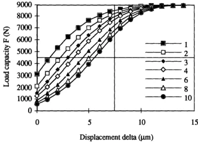
The load capacity changes with changing resistance ratio y, decreasing slightly with increasing y. Figure 3.13 shows a typical load capacity curve of a self-compensated bearing as function of displacement ( y=l to y=10). It has an effective bearing pad area

of 6140 mm2, a nominal bearing gap of 15 gm, a supply pressure of 10 atm and uses water as bearing fluid ( =0.001 Nsec./m2).

9000 8000 g 7000 v 6000 · 5000 4000 X 3000 2000 1000 0 0 5 10 15 Displacement delta (pm)

Figure 3.13: Load capacity of a self-compensated hydrostatic bearing.

Stiffness

The partial derivative of the load capacity with respect to the displacement delta is the stiffness and yields:

K=F d

(h-6)

_(h+6)

(h +8)

(h

+

)

3

(h -)3

+

(h

_-

)3

(h + 6)3'(h

_(h

+(h-

)

As for the load-capacity the stiffness change with changing . The effect is seen in Figure 3.14 for y=1 to =10. As the resistance ratio increases the stiffness gets more uniform for displacements . But for a displacement of 25 % of the nominal bearing gap the stiffness decreases, compared with the maximum value for y= 1.

I nn IL W 1000 800 2 600 400 200 0 5 10 15 Displacement delta (m)

Figure 3.14: Stiffness of a self-compensated hydrostatic bearing.

A lower stiffness may also be desirable to achieve a balanced design, preventing the bearing from being to stiff compared with the machine structure. With decreasing stiffness the damping capability of the bearing increases providing better dissipation of energy introduced by other machine elements.

4. Comparison of Self- and Fixed-Compensated Hydrostatic Bearings

Using the spreadsheets written for both types of bearings a comparison of hydrostatic bearings with fixed and hydrostatic bearings with self-compensation can be easily done by parameter studies. The two bearings analyzed are similar, distinguished only by the kind of compensation. The supply pressure is 10 atm, the bearing gap is 15 ptm and the bearing fluid used is water. Note that a bearing gap of 15 gm, and the use of water is desirable as described above but can only be realized using the principle of self-compensation. In order to analyze the differences between the compensation methods this is neglected.

The bearing parameters are:

supply pressure ps (atm,Pa= N/lm2) 10 1,013,250

ps (psi) 147

dynamic viscosity u [mu] (Nsec/mA2) 0.001

density p rho (kglm/3) 997

pocket depth hp (pm, m) 300 0.000300

nominal bearing gap h (pm, m) 15 0.000015

restrictorlbearing pad ratio 1

4.1 Load Capacity and Stiffness

Load capacity and stiffness of self-compensated hydrostatic bearings are approximately twice the value as for hydrostatic bearings with fixed compensation for a bearing/restrictor resistance ratio of 1. Figure 4.1/4.2 and Figure 4.3/4.4 show the load capacity and stiffness of this bearing configuration as a function of displacement . In order to provide a stiffness that has constant value over the range of displacement typically allowed in bearing applications, the bearing/restrictor resistance ratio should be about 3 to 4 with stiffness values still greater then for fixed compensated bearings.

It should be noted that increasing load capacity and stiffness of fixed compensated bearings to the level of self-compensated bearings by means of higher supply pressure results in higher pump power and therefore is not desirable.

6000 . 0 .9 5000 4000 3000 2000 1000 0 0 5 10 Displacement delta (pm)

Figure 4.1: Load capacity of a fixed-compensated hydrostatic bearing.

, .tt~' Yuuu 8000 7000 v 6000 * 5000 a 4000 , 3000 9 2000 1000 0 15 0 5 10 15 Displacement delta (m)

700 E =t Cn vD 600 500 400 300 200 100 0 0 5 10

Displacement delta (gim)

Figure 4.3: Stiffness of a fixed-compensated hydrostatic bearing.

1200 I: F. co a)i 403 1000 800 600 400 200 0 0 5 10 15 15 Displacement delta (nm)

Figure 4.4: Stiffness of a self-compensated hydrostatic bearing (Hydroguidem).

4.2 Manufacturing Error

The performance of hydrostatic bearings is to a large extent influenced by the nominal bearing gap. Therefore, with variations in bearing gap due to manufacturing errors the bearing is subjected to significant variations in performance. The actual bearing gap considers the error due to manufacturing errors and is described by the following equation:

hactual = hideal + error

The actual stiffness of the bearing is determined by implementing the actual bearing gap into the stiffness equation derived. The %-variation in stiffness is

(Kactual - Kideal)

%-variation in stiffness = 100

Kideal

with the ideal stiffness being the stiffness without manufacturing errors. Figure 4.5 and 4.6 show the %-variation in stiffness for a self- and a fixed compensated bearing as a function of manufacturing error for different nominal bearing gaps.

As seen in Figure 4.5 and 4.6 the self-compensated bearing shows a much smaller variation in stiffness for various manufacturing errors then the fixed compensated bearing. The latter is subjected to a significant loss in performance when the bearing gap varies due to manufacturing errors. Furthermore the restrictor resistance does not experience the same error and the resistance bridge becomes unbalanced. Therefore it requires careful hand-tuning of the flow restrictors to optimize performance. Self-compensated bearings are less sensitive to manufacturing errors and since bearing and restrictor pad experience exactly the same manufacturing error the resistance bridge stays balanced under all conditions and no hand-tuning is required.

This is especially important for decreasing nominal bearing gap, since smaller bearing gaps increase the performance and are in most applications preferred. The smaller the bearing gap becomes the less sensitive gets the self-compensated bearing while the %-variation in stiffness of fixed compensated increases.

.!U ? 10 o -10 -30 . -50 > -70 -90 -8 -4 0 4 8 Manufacturing error (gm)

Figure 4.5: Manufacturing error of a fixed-compensated hydrostatic bearing.

400 350 - 300 0 250 I, 200 .- 150 : 100 ' 50 0 -50 -8

Figure 4.6: Manufacturing error of

-4 0 4 8

Manufacturing error (pmn)

a self-compensated hydrostatic bearing.

-4.3 System Design

When designing hydrostatic linear motion bearings, requirements are often given in terms of stiffness and load capacity at a maximum displacement, maximum carriage velocity and available space for implementation. The bearing parameters have to be carefully chosen in order to achieve a good hydrostatic bearing complying with the specifications. Fixed and self-compensated bearings are discussed.

Supply Pressure

The supply pressure is determined by the desired load capacity and stiffness. Assuming that the bearing geometry is chosen the supply pressure can be varied according to the performance specifications. It is important to note the limits in supply pressure. First, higher supply pressure requires more pump power, resulting in an increase in temperature of the fluid. Furthermore, the higher the supply pressure the higher the pressure fluctuations introduced into the system. This is especially true for fixed compensated bearings with their low stiffness and load capacity values compared with self-compensated bearings. The supply pressure has to be significantly higher in this type of bearing.

Bearing Fluid

Normally used oil has the desired lubrication properties and is long term stable. It is used for fixed compensated bearings to make them work reliably. But oil has a high viscosity, limiting the reduction of the bearing gap and is environmentally unfriendly. Water, used in self-compensated bearings has a lower viscosity then oil and is environmentally friendly. In addition it has a higher heat capacity and excellent thermal conductivity. Lower viscosity reduces the necessary pump power and prevents the fluid film from building up hydrodynamic wedges at higher speeds. If water is used as a bearing fluid it should have biocidal and fungicidal additives. In addition, a water solvable lubricant may be added for increased pump life. Even it is theoretically possible to use water as fluid in fixed-compensated bearings, due to the compensation devices lack of self-cleaning this configuration is not used in practice.

Bearing Pad Geometry

The land width of linear hydrostatic bearings is typically 25% of the pad width but may have to be decreased for high speed applications in order to minimize the viscous shear and to prevent the bearing from running dry. The lands should always be large enough to support the weight of the carriage when the supply pressure is turned off. The pocket should be at least 10-20 times the nominal bearing gap for linear applications. When additional squeeze film land in the pocket are added, it must be assured that the bearing still can be lifted from rest and the water is evenly distributed to the bearing lands.

Nominal Bering Gap

The bearing gap in linear applications should be as small as possible, increasing load capacity, stiffness and damping and minimizing the required pump power. Smaller bearing gaps also increase the viscous shear generated in the bearing gap. However, linear application do not suffer from excessive heat generated through this effect due to relatively low speeds (30m/sec). The smallest nominal gap reasonable to manufacture is about 10 gm. Since fixed compensated bearings usually use oil as fluid the gap has to be larger than for self-compensated bearings. This results in decreased bearing performance.

Design for High Speed

For high speed applications for both bearing designs the same considerations apply. Careful calculations of the lowest fluid velocity in the bearing system have to be carried out in order to ensure that the fluid velocity is always larger than the carriage velocity. If the fluid velocity is too small, air is dragged into the bearing reducing the performance significantly. If necessary the fluid velocity can be increase by choosing a larger bearing gap to the detriment of load capacity and stiffness. The maximum speed of the carriage supported by a bearing with y=l and the smallest pocket pressure p is

ph2

In order to keep the fluid velocity high while a load is applied the bearing should experience zero displacement under these conditions maximizing the smallest bearing gap. This is achieved by unequally sized bearing pad. In addition, often the rail geometry requires unequally sized bearings, in order to utilize the entire width of the bearing rails and stiffness and load capacity requirements apply only in one direction. As a consequence the preload bearing pad can be of smaller dimension. In contrast to equally sized bearing pads, bearings having unequally sized bearing pads with the load bearing pad being larger than the preload bearing pad experience a displacement § opposite to the regular direction of loads when no load is applied. Since the smallest bearing gap determines the maximum allowable carriage velocity it is desirable to operate the system under load at zero displacement.

The negative displacement at zero load is due to the fact that the force of the load bearing pad is larger than the force of the preload bearing pad since ALoad > Apreload and PLoad =

PPrelaod.

FLoad = ALaod'PLoad > FPrelaod = APreloadPPreload

Thus, the bearing will be lifted, decreasing the preload bearing pad's flow resistance and pocket pressure and increasing the load bearing pad's flow resistance and pocket pressure until force equilibrium ALoad'PLoad = Apreload'PPrelaod is reached at a displacement. The average workpiece load, the minimum and the maximum load should be considered, reaching zero displacement for the load applied to the bearing.

Design for Low Power Generation

The total power of the hydrostatic system consist of the pump power and the friction power. Since the friction power is insignificant for linear applications the pump power has to be minimized. In order to reduce the required pump power the fluid flow must be minimized. This is achieved using small nominal bearing gaps providing larger flow resistances. Since load capacity and stiffness increase with decreasing gap the pump power

Design for Manufacturability, Assembly and Maintenance

Hydrostatic bearing pad geometries are easy to manufacture with a high degree of accuracy. Bearing gaps of 10-20 .tm, desired for high performance, can be manufactured with reasonable effort. In addition, hydrostatic bearing pads are self cleaning and can not be contaminated with dirt. This applies only for bearing pads. Restrictors are discussed separately

Fixed compensated bearings use flat-edge pins or capillary tube in order to provide the necessary restrictor resistance. Variation in the bearing gap due to manufacturing errors lead to the necessity of hand-tuning the resistance of the restrictor to the resistance of the bearing for maximum performance. This process, based on experience is time consuming and costly considering at least twelve bearing pads are used in machine tool application in order to restrict five degrees of freedom.

Fixed resistance resistors have very small diameter passages (ca. 0.4mm) that tend to clog during operation. Last chance filter screens have to be used to prevent the bearing from failing. Since capillary tubes and flat-edge pins are not self-cleaning they have to be disassembled from the machine for maintenance on a regular basis. Adjusting and maintaining fixed-compensated hydrostatic bearings is time consuming and cost intensive.

Self-compensated bearings are less sensitive to manufacture and require no hand-tuning since the resistance bridge remains balanced even with manufacturing errors introduced. The compensation device is self-cleaning and there are no smaller passages then 3-5 mm in diameter.