Reliability for fluid bearings design

Texte intégral

(1)Proceedings of the 19th ISSAT International Conference on Reliability and Quality in Design August 5-7, 2013 - Honolulu, Hawaii, U.S.A.. Reliability for Fluid Bearings Design K. Diop1, A. Charki1, S. Champmartin2, A. Ambari2 1. LASQUO-ISTIA, University of Angers, 62 avenue Notre Dame du Lac, 49000 Angers, France, [email protected] 2 LAMPA, Centre Arts et Métiers Paris Tech d’Angers, 2 boulevard du Ronceray, 49035 Angers Cedex, France. Keywords: Thrust Bearing, Fluid, Reliability, Monte Carlo, FORM Abstract - This paper presents a new methodology for evaluating the failure probability of fluid bearings which are sensitive components for the design of machine rotors, mechatronic systems and high precision metrology. The static and dynamic behavior of a fluid bearing depends on several parameters, such as external load, bearing dimensions, supply pressure, quality of the machined surfaces, fluid properties, etc. In this paper, the characteristics of a simple geometry thrust bearing are calculated analytically in order demonstrate the usefulness of the proposal methodology and its pertinence to bearing design. 1. Introduction Fluid bearings are vital components of machines used in mechanical engineering, where their purpose is to feed and guide the rotation of transmission shafts. They are found in rotating machinery such as compressors and turbines. Their main advantage resides in superior stiffness and stability compared with alternative bearing technology. For feeding rotors, hydrodynamic bearings (where the pressure gradient is generated simply by the relative movement of the rotor) do not provide adequate boundary lubrication during shutdown and start-up phases. To enable rotating machinery to handle large loads when rotor rotation speed is zero and guarantee a relative eccentricity close to zero, hybrid bearings are used (an external source, e.g. an orifice, generates additional pressure gradient) [1-3]. However, if these are not very carefully designed and optimized, their dynamic behavior can be unstable and at worst cause a catastrophic breakdown of a machine. It is therefore important when studying their reliability to take into account both static and dynamic characteristics (which depend on several parameters, such as bearing length and diameter, number of feed orifices and their diameters, rotation speed, etc.) [2,3]. A new methodology for reliable bearing design that takes the different influential factors into account is herein proposed. This paper examines the static characteristics of a circular thrust bearing in order to apply the methodology proposed for evaluating the failure probability of a bearing. 2. Reliability of a fluid bearing 2.1 Principle of reliability Reliability is a characteristic of a device expressed as the probability that it will accomplish a particular function under given conditions during a given time interval [4,5]. It can be deduced by estimating failure probability Pf.. Given the complexity of the failure domain and of the probability density function, which can bring into play a large number of variables, it is not easy to calculate the integral Pf, which is written as follow: 𝑃 =∫(. ). 𝑓. ,. ,…….,. (𝑋 , 𝑋 , . . , 𝑋 )𝑑𝑥 𝑑𝑥 , … , 𝑑𝑥 =. 𝑃𝑟𝑜𝑏{(𝐺(𝑋 )) ≤ 0}. (1). where G(Xi) is the performance function. When G(Xi) ≤0, one is in the domain of a space-variant failure probability with random variables. Aside from numerical integration methods, there exists today a comprehensive theorem on evaluation of this probability integral. This theorem includes: • An iso-probabilistic transformation of basic variables in a standard space where they become independent reduced centered Gaussian components. • The search in the standard space for a surface limit state design point P*, where the probability density is maximal. The failure probability is evaluated in the standard space using approximation methods. Figure 1 shows the transformation of physical space into normalized space. H is the equivalent of G in the normalized space. Failure probability is calculated analytically following transformation of physical space into normalized space with independent variables and determination of the failure point with the highest probability density - designated most probable failure point P*, see Figure 1.. Figure 1. Transformation of Physical Space into Normalized Space. The Monte Carlo method can therefore be applied but requires a long calculation time. Alternative methods based on approximation of the limit state function can be applied, such as the FORM (First Order Reliability Method) and SORM (Second Order Reliability Method) methods, for instance. A comparison of different approximation methods has been drawn up by Melchers [4] and Madsen [5]. These methods may be direct; make use of an optimization algorithm (the Rackwitz-Fiessler algorithm, for example); use response.

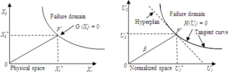
(2) surface method [3]. But above all, it is essential to define the performance function of the bearing being studied. 2.2 The Monte Carlo Method. 𝐼[𝐺(𝑋 ) ≤ 0]. (2). with Xi being the inth sample, and the indicator function I equal to 1 if the condition G(Xi) ≤ 0 is true and 0 if not. The evaluation of failure probability is accurate if the number of samples is sufficiently high. One of the major drawbacks of the Monte Carlo method is the high number of simulations required in certain cases. Indeed, for a low failure probability, an inadequate number of simulations could lead to a significant degree of error. 2.3 FORM method The FORM method (First Order Reliability Method) consists in estimating the reliability index β [5,6]. This method approximates the failure domain with a half-space delimited by a surface tangent hyperplane at design point P*, as shown in figure 1. Thanks to the rotational symmetry of the normalized multinormal distribution, the failure probability can be easily approximated by: 𝑃 = Ф(−𝛽). (3). where Ф is the standard normal distribution. Design point P* is determined by finding the limit state point closest to the origin of the normalized space. The design point is the solution of the following optimization problem: 𝛽 = 𝑚𝑖𝑛 √𝑼 𝑼 𝐻(𝑼) = 0. (4). where H is the equivalent of G in the normalized space (see Figure 1). U is the vector of random variables in the normalized space. This constrained minimization problem is resolved using the Rackwitz-Fiessler algorithm and the design point is evaluated as: 𝑼∗ = −𝜶 𝛽. (𝑼∗ ). (6). (𝑼∗ )‖. The reliability index β is then determined by:. Simulation methods make it possible to estimate the failure probability even when faced with complex laws of probability and non-linear correlations between variables or limit state functions. However, the calculation times required by these methods may be prohibitive. The principle of Monte Carlo simulations is to apply the law of probability to repeated samples conjointly with the random vector and count the number of times the system produces a result in the failure domain. The failure probability may be expressed by the following relation: 𝑃 ≈ ∑. 𝜶=‖. (5). The standardized gradient α of the limit state function, evaluated at design point U*, is determined by:. 𝛽=. (𝑼∗ ) ‖. (𝑼∗ )𝑼∗. (7). (𝑼∗ )‖. The tangent hyperplane equation (cf. figure 1) at design point U* is: 𝐻 (𝑼) = 𝛽 + ∑. 𝛼𝑢. (8). This method gives an accurate result when the limit state is linear in the standard space. It becomes inaccurate when the performance function is highly non-linear around the design point or when there are significant secondary minimums. 2.4 The Monte Carlo Method The performance function of a fluid bearing depends on the choice of different parameters, such as radii, the number of orifices, film thickness, feed pressure, etc. The failure probability of a fluid bearing is determined via the following performance function; this is defined as the difference between the load-bearing capacity corresponding to an operating thickness h, and the maximum load capacity corresponding to a critical level hc. 𝐺(𝑿) = 𝑊 (𝑿) − 𝑊. (𝑿). (9). where X is the vector of random variables, We-max is the maximum load capacity of the bearing, and We is the operating load capacity. The values for these two load capacities depend on the bearing parameters and are estimated by using the equations presented in the next section. Failure of a bearing occurs when the film thickness falls below critical thickness h c. 3. Modeling of a Fluid Bearing 3.1 Reynolds Equation Detailed explanations of how the simplifying assumptions were established for this study are given by Gross [1]: • The flow is continuous • The fluid is Newtonien • The flow is laminar and isothermal • The external mass forces and inertia force are negligible • There is no slippage between the fluid and the contact surfaces • The curvature of the fluid is ignored • The measured thickness of the fluid film is always small compared with the other dimensions of the contact area (indeed this is the underlying assumption of lubrication theory). • The velocity of one surface (surface 1) is tangent to that surface at all points (cf. figure 2), and given that.

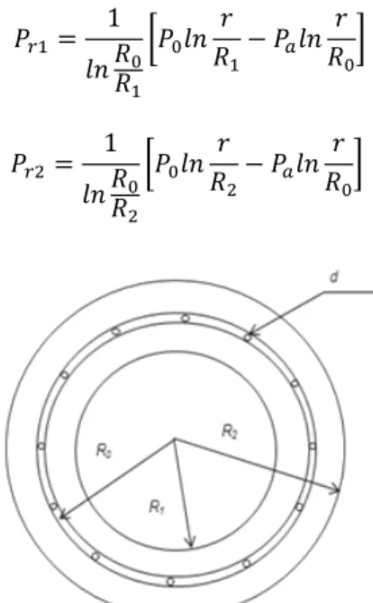
(3) specific gravity and viscosity do not vary with film thickness, the origin of the axes system is located at one of the contact surfaces. Figure 2 is a representation of the thin fluid film region. The projection is such that the z coordinate corresponds to film thickness. The velocity of a point on surface (1) is given by the U1, V1, W1 components and is related to the r, θand z coordinates. In the same way, the velocity of a point on surface (2) is given by the U2, V2, W2 components.. =0. (11). The pressure limit conditions are: 𝑟≤𝑅 ; 𝑃=𝑃 𝑟=𝑅 ; 𝑃=𝑃 𝑅 ≤𝑟≤𝑅 ; 𝑃=𝑃 𝑅 ≤𝑟≤𝑅 ; 𝑃=𝑃 𝑟=𝑅 ; 𝑃=𝑃 Integration of equation (11) with limit conditions gives the pressure expressions: 𝑃 =. 1 𝑟 𝑟 𝑃 𝑙𝑛 − 𝑃 𝑙𝑛 𝑅 𝑅 𝑅 𝑙𝑛 𝑅. 𝑃 =. 1 𝑟 𝑟 𝑃 𝑙𝑛 − 𝑃 𝑙𝑛 𝑅 𝑅 𝑅 𝑙𝑛 𝑅. Figure 2. Systems of Axes and Notation. Using the primitive equations for thin viscous films it is possible, with due regard for the geometric and kinematic conditions, to determine the thin film flow parameters, and in particular load-bearing capacity, flow-rate and stiffness. These equations can be deduced from the equations for continuous media mechanics applied to a Newtonian fluid [710]. Using the simplifying assumptions already cited, the conservation equations for the mass and momentum are obtained. Using the assumptions inherent to lubrication theory, the expressions for the fluid velocity components can be deduced relative to r and 𝜃 and in relation to the pressure gradient components and the velocity components at the surface (1). Integration along the velocity components axis (oz) of the conservation of momentum equation gives us the following Reynolds equation [1]: = 6𝑟𝜌(𝑈 − 𝑈 ). + 6𝜌(𝑉 − 𝑉 ) 6ℎ. + 6𝑟ℎ. +. [ 𝜌(𝑈 + 𝑈 )] +. [ 𝜌(𝑉 + 𝑉 )] + 6𝜌ℎ(𝑈 + 𝑈 ) + 12𝜌𝑟𝑊 +. 12𝑟ℎ. (10). 3.2 Practical Application to a Thrust Bearing In order to demonstrate our proposal methodology, we propose here to examine a simple example by applying Reynolds equation to a groove thrust bearing with feed orifices, as shown in figure 3. In this analytical study, the bearing is assumed to be symmetrical relative to angle θ and the feed pressure P0 is constant at radius R0. In the static case, the simplified Reynolds equation thus becomes:. Figure 3. Configuration of the Bearing Studied. Notation: P0: specific orifice supply pressure (Pa) Pa: atmospheric pressure (Pa), R1: inner radius (m), R0: orifice crown radius (m), R2: outer radius (m), r: elementary radius (m) ρ: fluid specific gravity (kg/m3) μ: dynamic viscosity (Pa.s), h: fluid film thickness between the upper and lower sides (m). 3.3 Performance function of Thrust Bearing Integration of surface pressure gives the load-bearing capacity expression, written as: 𝑊 = 𝜋(𝑅 − 𝑅 )𝑃 +. (. ). −. (12). This load-bearing capacity value may be determined relative to fluid film thickness h. For this, simply replace pressure P0 values with values obtained for different fluid film thicknesses h due to sustained volume flow rate. Integration of radial velocity at the rotor and stator transverse surface gives the.

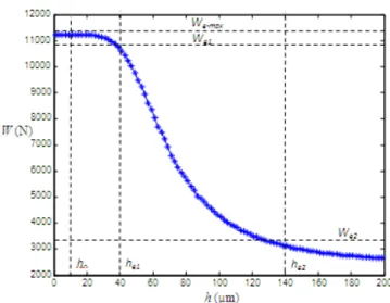
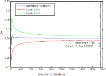
(4) expression for flow-rate through the bearing, and is written as follows: (𝑃 − 𝑃 ). 𝑄 =. +. (13). The input flow into the orifices is written thus: (. 𝑄 = 𝑛𝐶. ). (14). n: number of orifices Cd: discharge coefficient d: orifice diameter (m) PS: source pressure (Pa). The specific orifice supply pressure P0 is obtained by equalizing the input volume flow rate Q0 and the output volume flow rate QS. The performance function G for evaluating the failure probability is thus, 𝐺(𝑋) =. (. ). −. TABLE II. THRUST BEARING RANDOM VARIABLES Variables. Mean. CV. Distribution. R1 (mm). 30. 10%. Normal. R0 (mm). 48. 10%. Normal. R2 (mm). 75. 10%. Normal. d (mm). 0.15. 10%. Normal. Figure 4 shows changes in load-bearing capacity W relative to fluid film h obtained from expression (12). For the evaluation of failure probability of the bearing studied, we assume that hc = 10 µm and we consider two operating load capacities We1 = 1.0572 E+04 N and We2 = 3.1777 E+03 corresponding to respectively two fluid thickness he1= 40 μm and he2= 140 μm. The maximum load capacity We-max = 1.1236 E+04 N is obtained for hc.. (15). where 𝑃 and 𝑃 are respectively the pressure P0 calculated for the thickness fluid film h and hc using the expressions (13) and (14). The performance function G can be evaluated by using the vector of random variables X = {µ, ρ, Cd , d, PS, R1, R2, R0). 4. Application Let us now consider the thrust bearing described in paragraph 3.2. The thrust bearing parameters used for calculations are shown in table I. Table II shows the variables used for estimating failure probability. This table gives the mean, the coefficient of variation (CV), and the associated distribution law for each variable. TABLE I. THRUST BEARING PARAMETER VALUES Designation. Value. R1 (mm). 30. R0 (mm). 48. R2 (mm). 75. ρ (kg/m3). 794.7. Pa (Pa). Figure 4. Load Bearing Capacity versus Fluid Thickness. Table III shows the results obtained with the Monte Carlo and FORM methods for two operating load bearing capacities We1 and We2 corresponding to two respective operating thicknesses he1 and he2. The estimation of Pf for the two operating load capacities We1 and We2 is calculated with We-max = 1.1236 E+04 N using the performance function (15). The probability of failure diminishes as fluid film thickness increases; it also diminishes as nominal load capacity gets further from critical load capacity. TABLE III. FAILURE PROBABILITY WITH FORM AND MONTE CARLO. 5. 10. 5. Method. Probability Pf. Time (s). FORM (he1 = 40 µm). 0.06120. 15.5. Ps (Pa). 5.10. FORM (he2 = 140 µm). 0.00251. 182. d (mm). 0.15. Monte Carlo (he1 = 40 µm). 0.05356. 495.59. Cd. 0.7. Monte Carlo (he2 = 140 µm). 0.00124. 34493. μ (Pa.s). 0.0012. n (number of orifices). 12. Figures 5 and 6 give an estimation of failure probability Pf with the Monte Carlo method for he1 = 40 µm and he2 = 140 µm. The results of Pf are obtained with a confidence interval of 95%. As shown in figures 5 and 6, the results converge.

(5) giving a coefficient of variation of CV = 0.1 for the Pf values. It is clear that the calculation is very long using the Monte Carlo method, especially for very low failure probabilities, as shown in table III. FORM remains a useful tool for the failure probability estimation of a bearing.. The results obtained using the FORM and Monte Carlo methods suggest that the methodology developed here is worth exploring with other configurations, for instance with a larger number of variables. FORM, as is explained in the literature, is advantageous from the point of view of calculation times. The non-linear limit function of G can also be approximated using SORM (Second Order Reliability Method) and the error of approximation can also be analyzed for all proposal methods in this article. The methodology expounded here is applied in the LASQUO and LAMPA laboratories for other types of bearings (cylindrical, etc.). 6. References [1] Gross, W. A., Matsch, L. A, Castelli, V., Eshel, A., Vohr, J. H., Wildmann, M., “Fluid Film Lubrication”, John Wiley and Sons, New York, 2008.. Figure 5. Failure Probability for he1 = 40 µm. [2] Charki A., Bigaud D.,Guerin F., “Behavior Analysis of Machines and System Air, Hemispherical Sprindles using Finite Element Modelling”, Industrial Lubrication and Tribology, Vol. 65. 2013 [3] Charki A., Elsayed E. A., Guerin F., Bigaud D., “Fluid thrust bearing reliability analysis using finite element modeling and response surface respond”, International Journal of Quality Engineering and Technology, Vol. 1, pp. 188-205, 2009. [4] Madsen H. O., Krenk S., Lind N. C., “Structural method of safety”, Prentice-Hall, Upper Saddle River, New Jersey, 1986. [5] Melchers R. E., “Structural reliability analysis and Prediction”, Second Edition. John Wiley and Sons, New York, 1999. [6] Di Sciuva M., Lomario D., “A comparison between Monte Carlo and FORMs in calculating the reliability of a composite structure”, Composite structures, Vo. 59, pp. 155162, 2003.. Figure 6. Failure Probability for he1 = 140 µm. 5. Conclusion In this paper, we present a new methodology that is of practical use in bearing design. The approach developed here demonstrates the value of estimating failure probability and shows how bearing design may be optimized via reliability criteria. A simple application is used to illustrate the argument, that of a thrust bearing fed with a pressure source via orifices. To calculate the failure probability of the bearing, two operating load capacities are examined, one of which is close to the critical load capacity associated with the minimum thickness below which the bearing cannot function, while the other is nowhere near the critical load capacity. Failure probability increases as the fluid film value decreases.. [7] Dennis V. De Pellegrin, Douglas J. Hargreaves, “An isoviscous, isothermal model investigating the influence of hydrostatic recesses on a spring-supported tilting pad thrust bearing”, Tribology international, Vol. 51, pp. 25-35, 2012. [8] Jang G. H., Kim Y. J., “Calculation of dynamic coefficients in a hydrodynamic bearing considering five degrees of freedom for a general rotor-bearing system”, Journal of Tribology, Vol. 121, pp. 499-505, 1999. [9] Srikanth D. V., Kaushal Chaturvedi K., Chenna Kesava Reddy A., “Determination of a large tilting pad thrust bearing angular stiffness”, Tribology International, Vol. 47, pp. 69-76, 2012. [10] Charki A., Diop K., Champmartin S., Ambari A., “Numerical simulation and experimental study of thrust air bearings with multiple orifices”, International Journal of Mechanical Sciences, 2013..

(6)