Design and manufacturing of modular self-compensating hydrostatic journal bearings

by

Markku Sami Antero Kotilainen S.M., Mechanical Engineering Helsinki University of Technology, 1997

SUBMITTED TO THE DEPARTMENT OF MECHANICAL ENGINEERING IN PARTIAL FULFILLMENT OF THE DEGREE OF

DOCTOR OF PHILOSOPHY at the

MASSACHUSETTS INSTITUTE OF TECHNOLOGY June 2000

© 2000 Massachusetts Institute of Technology All rights reserved

Signature of Author ...

Certified by ... ..

Accepted by... ...

Department of Mechanical Engineering June 2, 2000

Alexander H. Slocum Professor of Mechanical Engineering Thesis Supervisor

...

Ain A. Sonin Professor of Mechanical Engineering Chairman, Committee for Graduate Students

MASSACHUSETTS INSTITUTE OF TECHNOLOGY

SEP 2 02000

Markku Sami Antero Kotilainen

Submitted to the Department of Mechanical Engineering on July 2, 2000 in Partial Fulfillment of the

Requirements for the Degree of Doctor of Philosophy in Mechanical Engineering at the Massachusetts Institute of Technology

ABSTRACT

In order to carry a load, a multi recess hydrostatic bearing supplied with a single pressure source requires compensation devices. These devices are also known as restrictors and they allow the recess pressures to differ from each other. These devices, when properly selected and tuned, can deliver excellent bearing performance. However, these devices add to the complexity of the bearing and they are sensitive to manufacturing errors. These devices must often be tuned specifically for each bearing and are therefore expensive to install and maintain.

Self-regulating or self-compensating bearings do not need any external devices to achieve load-carrying capability and they do not add to the total degrees of freedom of the system. However, in many cases the proposed designs require multiple precision manufacturing steps such as EDM and grinding in addition to precision shrink fit.

In this work a self-compensating design, which eliminates all but one precision-manufac-turing step, was manufactured and tested. Novel manufacprecision-manufac-turing methods for different sizes were introduced. The test results were compared with theoretical results and satisfactory agreement was achieved. The bearing sensitivity to manufacturing errors was analyzed computationally using statistical methods. These results were used to show that the intro-duced manufacturing methods are more cost effective than the applicable precision or semi precision manufacturing methods even when the performance variation is taken into account.

When hydrostatic journal bearing is rotated hydrodynamic effects are introduced. Often, these effects are ignored by assuming them to be insignificant. Two non-dimensional parameters were derived to estimate the significance of the hydrodynamic effects and lim-its to these parameters were searched numerically. Design theory, along with first order equations to estimate bearing performance was developed.

Thesis Supervisor:

Professor Alexander H. Slocum

First and foremost, I would like to thank my wife, Paivi. Who followed me here and unconditionally supported and loved me. No words or thank you can ever do justice to what you have done for me. Tama on sinulle oma pikku sipulini.

I would like to thank my always inspirational advisor Prof. Alex Slocum, who's endless energy, amazing creativity, knowledge and wisdom are without parallel. It was great learn-ing from you, I could not have had a better advisor. I would also like to thank the rest of my thesis committee, Professors David Trumper and Samir Nayfeh, who were always sup-portive and helpful.

I would also like to thank my dad for his support and advice.

I would also like to thank the following foundations for making this endeavour financially possible: Walter Ahlstromin saatii, Jenny ja Antti Wihurin rahasto, Alfred Kordelinin saitio, Thanks to Scandinavia foundation, Suomen Kulttuurirahasto and Suomen Akatemia. Thankfully, Sami Kotilainen June 2. 2000 Cambridge, Massachusetts 5

Acknowledgments ... Nomenclature ...

Chapter 1. Introduction . . . . 1.1 Scope of the Thesis . . . . 1.2 Background . . . . 1.2.1 Bearing Technology . . . 1.2.2 Hydrodynamic Bearings . 1.2.3 Hydrostatic Bearings . . .

Chapter 2. Surface Self-compensation . . . . 2.1 Surface Self-Compensating Hydrostatic Bearings 2.2 Why Bushing? . . . .

Chapter 3. Modeling . . . .

3.1 Lumped Parameter Modeling . . . .

3.1.1 Validity of the Geometric Assumption . . .

3.1.2 Example Lumped Parameter Model . . . .

3.2 Finite Difference Modeling . . . . 3.2.1 Bearing Geometry Generation . . . . 3.2.2 Validity of the Finite Difference Solution

3.2.3 Turbulence Modeling . . . .

Chapter 4. Analytical Considerations . . . .

4.1 Static characteristics of a plain journal bearing . .

4.1.1 Infinitely long bearing . . . .

4.1.2 Short bearing . . . . 4.2 Dynamic coefficients of a plain journal bearing

4.2.1 Derivation of the dynamic coefficients . 4.2.2 Infinitely Short Bearing . . . .

4.2.3 Infinitely Long Bearing . . . .

4.3 Fixed Restrictor Deep-Pocket Hydrostatic Bearing 4.4 Bearing Stability . . . .

..

Design . . . .

5.1 General Considerations . . . .

5.2 Low (laminar) Speed . . . .

5.2.1 Summary of Laminar Design Issues 5.3 High Speed (Turbulent) . . . . 5.4 Adjustable Clearance and Shape . . . . .

5.5 Summary of Design . . . . . . . . 95 . . . . 9 5 . . . 104 . . . 12 8 . . . 12 8 . . . 136 . . . 14 2 Chapter 6. Manufacturing . . . .

6.1 Selecting a Manufacturing Method . . . . 6.2 Manufacturing of the 6" Prototype Bushing . . . . 6.2.1 Shrinkage and Dimensional Variation . . . . 6.2.2 Run-Test of Groove Width Measurement Data . 6.2.3 Chi-Square () Test of Groove Width Measurement 6.3 Manufacturing of the 1.25" Prototype Bushing . . . . .

6.3.1 Problems with 1.25" Prototype Manufacturing 6.3.2 Solutions to Manufacturing Problems . . . . 6.3.3 Shrinkage and Dimensional Variation . . . . 6.4 Sensitivity of the Bearing to Manufacturing Errors . . . 6.4.1 M odel . . . . 6.4.2 The Effect of Manufacturing Errors on Load Capa 6.4.3 Cost vs. Quality Analysis . . . .

city

Chapter 7. Testing . . . . 7.1 Static Testing of the 6" Prototype . . . . 7.1.1 Test Set-up . . . . 7.1.2 Results . . . . 7.1.3 Conclusions . . . . 7.2 Dynamic Stiffness Testing of the 6" Prototype

7.2.1 Test Set-up . . . . 7.2.2 Results . . . . 7.3 Static Testing of the 1.25" Prototype . . . . . 7.3.1 Test Set-up . . . . 7.3.2 Results . . . . 7.3.3 Conclusions . . . . 7.4 Error Motion Measurements . . . .

. . . 17 9 . . . 17 9 . . . 18 0 . . . 18 7 . . . 19 6 . . . 19 7 . . . 19 7 . . . 19 8 . . . 2 0 0 . . . 2 0 0 . . . 2 0 3 . . . 2 0 4 . . . 2 0 5 Data 145 145 148 150 153 154 157 158 160 160 162 162 164 171

7.4.3 Results . . . . 7.4.4 Conclusions . . . . Chapter 8. Applications . . . . 8.1 G eneral . . . . 8.2 TurboTool . . . . 8.2.1 Preliminary Analysis of TurboTool Concept . . . 8.3 Conceptual Very Small Machine Tool . . . . 8.3.1 Functional Requirements for Small 5-Axis Machine 8.3.2 Concept Selection . . . . 8.3.3 Concept Feasibility . . . . 8.4 Sealing . . . . Chapter 9. Conclusions and future work . . . . References . . . . Appendix A. Automatic Geometry Generation . . . . Appendix B. Data analysis for error motion measurements . Appendix C. Wobble Plate . . . . Appendix D. TurboTool Appendix E. . . . . 208 . . . 212 . . . 213 . . . 213 . . . . 214 . . . 215 . . . . 221 . . . . 221 . . . . 225 . . . . 225 . . . . 232 . . . . 237 . . . . 241 . . . . 245 . . . . 275 . . . . 281

Finite element program to solve linearized dynamic response of the .... ... . . . .. 283

Figure 1.2 Hydrostatic double- or opposed pad bearing and pressure diagrams. 27

Figure 1.3 Hydrostatic bearing electric circuit analogy . . . . 27

Figure 1.4 Spool valve compensators . . . . 30

Figure 1.5 a) Diaphragm restrictor b) Diaphragm as a flow divider . . . . 31

Figure 1.6 Shallow recess hydrostatic bearing . . . . 32

Figure 2.1 Surface self-compensating linear bearing [Slocum, 1992]. . . . . 36

Figure 2.2 Normalized load capacity and stiffness of self-compensating bearing. Nor-malized by fixed restrictor bearing. . . . . 38

Figure 2.3 Cross sectional and developed view of surface self-compensating journal bearing . . . . 39

Figure 2.4 Developed view of surface self-compensating bearing . . . . 39

Figure 2.5 Surface self-compensating journal bearing with deterministic compensators [Slocum , 1994] . . . . 40

Figure 2.6 Surface self-compensating bearing with cross drilled collectors and load pockets on shaft . . . . 41

Figure 2.7 Bearing design with all the geometry on the shaft surface . . . . 41

Figure 3.1 Circumferential flow over land in displaced journal bearing . . . . 44

Figure 3.2 Ratio between full solution and flat plate approximation in case of circum-ferential flow in a journal bearing . . . . 46

Figure 3.3 Ratio between full solution and flat plate approximation in case of axial flow in a journal bearing . . . . 47

Figure 3.4 Lumped parameter model . . . . 47

Figure 3.5 Equivalent circuit . . . . 48

Figure 3.6 Finite difference grid . . . . 51

Figure 3.7 a) Too coarse mesh results in wider than real grooves, b) Points close to groove edge result in better interpolation of real geometry . . . . 54

Figure 3.8 Groove depth test case . . . . 55

Figure 3.9 Bearing force as function of eccentricity ratio . . . . 58

Figure 3.10 Variation of the recirculation pressure gradient with groove depth . . . 59

Figure 4.1 Co-ordinate system . . . . 66

Figure 4.2 Non-dimensional load for the different assumptions . . . . 68

Figure 4.4 Figure 4.5 Figure 4.6 Figure 4.7 Figure 4.8 Figure 4.9 Figure 4.10 Figure 4.11 Figure 4.12 Figure 4.13 Figure 4.14 Figure 4.15 Figure 4.16 Figure 4.17 Figure 5.1 Figure 5.2 Figure 5.3 Figure 5.4 Figure 5.5 Figure 5.6 Figure 5.7 Figure 5.8 Figure 5.9 Figure 5.10 Figure 5.11 Figure 5.12 Figure 5.13

Section showing bearing co-ordinate system . . . . 70

Intermediate bearing co-ordinate frame . . . . 72

Pressure given by Equation 4.41. . . . . 77

Change of basis . . . . 78

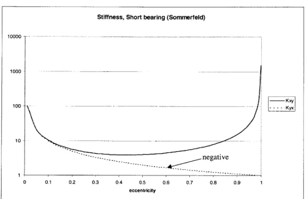
Stiffness coefficients for infinitely short bearing with Sommerfeld's condi-tions . . . . 79

Damping coefficients for infinitely short bearing with Sommerfeld's condi-tions . . . . 79

Stiffness coefficients for infinitely short bearing with Gumbel's conditions 81 Damping coefficients for infinitely short bearing with Gumbel's conditions 82 Pressure given by Equation 4.56. . . . . 83

Stiffness coefficients for long bearing with Sommerfeld's conditions . 85 Damping coefficients for long bearing with Sommerfeld's conditions . 85 Stiffness coefficients for long bearing with Gumbel's conditions . . . 87

Damping coefficients for long bearing with Gumbel's conditions . . . 87

Typical fixed restrictor hydrostatic bearing . . . . 89

Sensitivity of initial pressure ratio to manufacturing errors . . . 102

Sensitivity to clearance errors. . . . 103

Design parameter relation to bearing geometry . . . 104

as function of resistance ratio . . . 106

Removing central lands to improve high speed frictional characteristics 109 Normalized A* for laminar flow . . . .111

Normalized A* for transitional flow . . . 112

Normalized A* for turbulent flow . . . 112

Pressure formation in converging gap . . . 113

Converging gap divided into sections . . . 115

Ratio between uninterrupted and interrupted hydrodynamic force . . . 116

Coordinate system for the 2.35" bearing results . . . 119

Pressure distribution for the grooved and plain bearing with supply pressure () . . . 120

Figure 5.15 Figure 5.16 Figure 5.17 Figure 5.18 Figure 5.19 Figure 5.20 Figure 5.21 Figure 5.22 Figure 5.23 Figure 5.24 Figure 5.25 Figure 6.1 Figure 6.2 Figure 6.3 Figure 6.4 Figure 6.5 Figure 6.6 Figure 6.7 Figure 6.8 Figure 6.9 Figure 6.10 Figure 6.11 Figure 6.12 Figure 6.13 Figure 6.14 Figure 6.15 Figure 7.1 Figure 7.2

Bearing force for different 2.35" bearing cases . . . 121

Hydrodynamic force of the grooved bearing and the short bearing approxi-mation divided by the . . . 122

Pressure distribution for a bearing with high power ratio (38) () . . . . 124

Pressure distribution for a bearing with high power ratio (25)

0

Pressure distribution for a bearing with high power ratio (40) () and central lands rem oved . . . 126

Simple step bearing . . . 127

Pressure distribution for a high speed (100 000 rpm) bearing . . . 130

Pressure distribution for laminar design at 100 000 rpm . . . 132

Pressure distribution for SC5 design at 100 000 rpm . . . 134

Pressure distribution for SC6 small recess design at 100 000 rpm. . . 135

Cylinder with internal and external pressure . . . 138

Stereolithography negative of grooving geometry . . . 149

A) Core-box, B) Sand core in the mold . . . 150

A) Cast bushing, B) Groove detail . . . 150

The measured and normal distributions for groove width data . . . 156

A) 3D-Printed wax pattern, B) Investment cast part . . . . Problems with printing deep grooves . . . . Lumped parameter discretization . . . .... Bearing force distribution with ecc=0.1, % of land width Force angle distribution with ecc=0. 1, % of the land widths Bearing force distribution with ecc=0.5, % of land width Bearing force distribution with ecc=0. 1, % of groove width Loss function concept . . . . The derivation of expected cost . . . . Normalized manufacturing cost as function of quantity . Normalized manufacturing cost as function of quantity . General view of the test setup . . . . Bearing assembly and the location of the capacitance probes . . . 157 . . . 159 . . . 163 . . . 165 . . . 166 . . . 169 . . . 170 . . . 172 . . . 173 . . . 176 . . . 177 . . . 180 . . . 182

Figure 7.3 Figure 7.4 Figure 7.5 Figure 7.6 Figure 7.7 Figure 7.8 Figure 7.9 Figure 7.10 Figure 7.11 Figure 7.12 Figure 7.13 Figure 7.14 Figure 7.15 Figure 7.16 Figure 7.17 Figure 7.18 Figure 7.19 Figure 7.20 Figure 7.21 Figure 7.22 Figure 7.23 Figure 7.24 Figure 7.25 Figure 7.26 Figure 7.27 Figure 7.28 Figure 8.1

Photograph of the test setup . . . 183

Bearing assem bly . . . 185

Reaction forces on the shaft in the case that both bushings have the same geom etry . . . 186

Gap test. Pump turned off and on while measuring the displacement. . 187 Uncorrected force-displacement curves at 250 psi measured with the 50k force transducer . . . 188

3D Finite element model . . . 190

Displacement of the test setup with 10 OOON load . . . 191

The simplified beam model . . . 192

Beam model displacement . . . 192

Corrected force-displacement curves at 250 psi with 50k force transducer. (CorrI=corrected results of the probe 1, Corr2=corrected results of the probe 3)... ... 193

Corrected force-displacement curves at 250 psi supply pressure and the 5k force transducer. (Corr =corrected results from probe 1, Corr3=corrected results from probe 3) . . . 195

Impact and acceleration measurement points . . . 197

The dynamic stiffness and phase traces for the points 1,2 and 5. . . . . 199

Simple single d.o.f system . . . 199

General and side view of the test set-up. General view is rotated upside down for clarity. . . . 201

Photograph of the test set-up . . . 201

Bearing assembly . . . 202

Force displacement results at 500 psi. . . . 203

Two gauge method with offset spherical master . . . 206

The error motion test set-up. . . . 208

Error motion test set-up (2" ball) . . . 208

Error motion trace for single revolution . . . 209

Error motion for multiple revolutions . . . 209

Asynchronous error motion . . . 210

Noise level with pump on . . . 211

Noise without the pump . . . 212 . . . . 2 15

Figure 8.3 Figure 8.4 Figure 8.5 Figure 8.6 Figure 8.7 Figure 8.8 Figure 8.9 Figure 8.10 Figure 8.11 Figure 8.12 Figure 8.13 Figure 8.14 Figure 8.15

Transfer function for the tool tip displacement of the TurboTool Typical gantry type arrangement of axis . . .

Hexapod (Steward platform) . . . . Linear-rotary concepts (actuators not shown) . Circular concept . . . . Double yoke design . . . . Finite element representation of the lower yoke Transfer functions for the lower yoke . . . . . Slinger seal . . . . Labyrinth seal . . . . Clamped circular flat plate . . . . Combination of slinger, lip and air barrier seal Combined air barrier lip seal . . . .

. . . 221 . . . 223 . . . 224 . . . 225 . . . 225 . . . 228 . . . 230 . . . 231 . . . 233 . . . 234 . . . 235 . . . 236 . . . 236

TABLE 3.2 TABLE 3.3 TABLE 3.4 TABLE 3.5 TABLE 3.6 TABLE 5.1 TABLE 5.2 TABLE 5.3 TABLE 5.4 TABLE 5.5 TABLE 5.6 TABLE 5.7 TABLE 5.8 TABLE 5.9 TABLE 5.10 TABLE 6.1 TABLE 6.2 TABLE 6.3 TABLE 6.4 TABLE 6.5 TABLE 6.6 TABLE 6.7 TABLE 6.8 TABLE 6.9 TABLE 6.10 TABLE 6.11 TABLE 6.12 TABLE 7.1

Pm for different groove depths and diameters ... ... 56

Initial pocket pressure ratios for the two models ... 57

Dimensions for the two different test cases .... ... 61

Comparison of flow rates for Case #1 ... 61

Comparison of flow rates for Case #2 . . . . 62

Non-dimensional parameters for different bearing geometries and types [W asson, 1996] . . . . 98

Flow regimes for different bearing regions . . . 105

Minimum film thickness for different bearing sizes and surface speeds 110 Maximum allowable surface pressures for different bearing materials 110 Main dimensions of 2.35" bearing . . . 118

Summary of the computed results . . . 119

Comparison between finite difference computed and derived estimated val-ues ... ... 123

Dimensions of 100 000 rpm bearing . . . 130

Summary of different high speed cases (100 000 rpm) . . . 132

Summary of the high speed designs (100 000 rpm) . . . 136

Possible bushing manufacturing methods . . . 146

Diameter Measurements of 6" Bushings . . . 152

Groove Width Measurement Statistics . . . 153

Chi-Square Test for Groove Width Measurement Data . . . 156

Measurement statistics of the first two sets of 3D-printed parts . . . . 161

Measurement statistics of the sets III and IV of 3D-printed parts . . . 161

Summary of the results for % of the land widths case . . . 166

Summary of the results for % of the groove width case . . . 167

Summary of the results for % of the land widths case . . . 167

Summary of the results for % of the land widths case . . . 167

Summary of the results for % of the land widths case . . . 168

Summary of the results for % of the land widths case . . . 169

TABLE 7.2 TABLE 7.3 TABLE 7.4 TABLE 7.5 TABLE 8.1 TABLE 8.2 TABLE 8.3 TABLE 8.4 TABLE 8.5 TABLE 8.6

Initial Stiffness at 250 psi . . . 195

Flow rate at 500 psi . . . 196

Initial stiffness of the 1.25" prototype . . . 204

Measured and predicted flow for the 1.25" bearing . . . 204

Bearing dimensions for TurboTool . . . 217

Bearing properties at equilibrium point under maximum machining force 218 Concept selection . . . 226

Geometric error gains . . . 228

Static stiffness of the double yoke concept . . . 229

A area [m2

A; Routh-Hurwitz coefficient A* equivalent friction area

B,b damping coefficient [Ns/m]

c heat capacity []

Cf friction factor

C clearance [in]

D diameter [m]

e radial displacement [in]

E Young's modulus [Pa]

f

Ff force [N]

fr friction factor

g gravitational acceleration [m/s2]

h film thickness [in]

i current [A]

I _{second moment of inertia [m}4_] K,k stiffness [N/m]

L length [m]

M,m mass [kg]

N rotational speed [rev/min]

NTa Taylor number

n shear stress ratio, index P,p pressure [Pa], power [W]

Q

R radius [m]

R; flow resistance [Pa/m3/s]

Re Reynolds number S Sommerfelds number T torque [Nm] u, U velocity [m/s], displacement [m] V volume [m3] W load [N] w width [m] displacement (small) [m] E strain, eccentricity hydraulic resistance ratio

y angle between pocket and restrictor [rad]

X scale factor

viscosity [Pa s], mean value

H power ratio

' pumping ratio

p density[kg/m3]

(Y stress [Pa]

V Poisson's ratio

shear stress [Pa] attitude angle [rad] wo rotational speed [rad/s]

INTRODUCTION

This chapter includes an introduction to this thesis. It is also intended to serve as an short introduction to bearing technology in general and specifically to non-contact fluid film bearings.

1.1 Scope of the Thesis

The purpose of this research is to create a fundamental new machine element: a modular hydrostatic bushing. In this research, a design theory for conformable surface self-com-pensating hydrostatic bushing bearings is be developed and then be to design and manu-facture surface self-compensating hydrostatic bushing bearings. The design is divided into three distinct sections: low-speed design, high-speed design and conformability. Two dif-ferent designs and sizes are manufactured and tested and compared to calculated values. Analytical, lumped parameter and finite difference approaches are used to model the bear-ing behavior. The validity of different models are discussed. Different manufacturbear-ing methods are compared by means of statistical model which models the effect of manufac-turing errors on the bearing performance. A cost-function approach [Taguchi, 1989] is used to derive a single measure which is then used to compare the different methods. Dif-ferent applications such as a very small machine tool, high speed milling spindle and lin-ear-rotary axis are discussed.

This thesis will attempt to make the following fundamental contributions: -Incorporate surface self-compensation technology into a bushing bearing

Surface self-compensating bearings offer great advantages over traditional hydrostatic bearings. They utilize surface geometry for metering the fluid flow (compensation), col-lecting the fluid and channeling the fluid to the opposite side of the bearing to a pocket region. This design does not use capillaries or diaphragms to achieve load compensation. Everything needed is included in the surface geometry of the bearing. This research will incorporate this technology into a cast or molded bushing bearing to create a versatile and robust hydrostatic bearing. [Slocum, 1992,Wasson, 1996].

-Find economically viable manufacturing methods for the bearing

Manufacturing the bushings is by no means a trivial task because of the fluid circuitry required by the self-compensation.

- Model the bearing performance in the presence of manufacturing and other errors

Different manufacturing methods have different natural variations associated with the accuracy they can produce. These manufacturing errors can be best described in statistical terms because of their inherent randomness. Monte-Carlo and cost function approach is used to derive a single numeric value which can be used to determine the total expected cost of the bearing. By using this measure to perform the comparison between different manufacturing methods, the comparison becomes more analytic.

- Design adjustable-gap hydrostatic bushing bearing

Self-compensation allows the bearing gap to be changed without changing the designed properties of the bearing. The possibility to adjust the bearing gap is attractive because it allows the adjusting of the flow rate and pumping power and also introduces a possibility to use larger manufacturing tolerances.

Complement the design theory of surface self-compensated bushings by studying the effect of hydrostatics on journal bearing stability.

Hydrostatic bearing stability is investigated using computational methods at high speed. The possibility to use hydrostatics to enhance the stability of a journal bearing is researched. Different high speed designs are proposed. The shape of the bushing surface can also be designed to enhance the stability [Frene, 1990]. The possibility to conform the bushing to enhance stability will be discussed.

1.2 Background

This section discusses shortly different types of bearings and their applications. First a very general look into bearing technology is taken and then a little more detailed look is taken into fluid film bearings in general and more specific introduction to hydrostatic bearing follows.

1.2.1 Bearing Technology

Bearings are among the most important mechanical machine elements. Their main func-tion is to guide mofunc-tion and carry load. Other requirements are be speed-, accelerafunc-tion-, range of motion, stiffness, damping, accuracy, friction, thermal requirements, environ-mental requirements, size, life time and cost. As broad as are the requirements is the selec-tion from which a designer can select a device to fulfill them. Bearings can be categorized in many ways, the broadest maybe being the division into contact and non-contact bear-ings. Contact bearings can be further divided into sliding contact, rolling element and flex-ural bearings. Non-contact bearings include hydrostatic, hydrodynamic, aerostatic and magnetic bearings. All of the above mentioned general types include multiple sub-types or variations. Already it is obvious that the selection is enormous and very specific set of requirements must be formed to end up with an optimum type for a certain application. Comparison in general terms is not possible or fair, since the performance characteristics are so varied. The requirements of the specific application determines the weight of the

different desired qualities and only then the best possible solution for those weights can be found. For example, in machine tool spindles rolling element-, hydrodynamic-, air-, mag-netic- and hydrostatic bearings are used. This example proves that even for fairly specific application, machine tool spindle, the choice is far from obvious. In this thesis some com-parisons are made and it must be noted that comparison always refers to a certain subset of requirements and should not be generalized.

Next a bit more detailed look is taken into two types of non-contact bearings, namely the hydrodynamic and hydrostatic bearings.

1.2.2 Hydrodynamic Bearings

Hydrodynamic bearings form their load carrying capacity by the pressure rise in a con-verging oil film. This requires relative motion between the surfaces and the surfaces not being parallel. The reason why hydrodynamic bearings are introduced in this thesis is that the hydrodynamic effect also exists in hydrostatic bearings with varying magnitude and importance. Chapter 4 formulates analytical solutions to the hydrodynamic bearing to demonstrate and approximate its effect on hydrostatic bearing performance.

Hydrodynamic bearings are used as both thrust and journal bearings and in combination. There exists many variations and shapes such as partial arc, full arc, lobed, herring bone and tilting pad hydrodynamic bearings. Different geometrical features or pressurized oil supply can be implemented to make sure load carrying oil film exists everywhere.

Hydrodynamic bearings have many desirable properties. They are self-acting and do not need external sources to operate, they have long life when used properly, they are robust, have high stiffness, damping and load capacity. In some cases they have undesirable prop-erties such as the relative motion required between the surfaces (stop and go applications), instability at high speeds (half frequency whirl), relatively large eccentricities required to achieve load capacity, high viscous drag at high speeds and high temperature rise due to that. Many of these features can be diminished or eliminated by using certain designs, for

example tilting pad bearings are stable (against whirl) at all operating speeds. Naturally there are trade offs between different desired properties and implemented design features. To learn more about hydrodynamic bearings the reader is referred to Chapter 4 or [Frene,

1990].

1.2.3 Hydrostatic Bearings

Hydrostatic bearings are non-contact bearings which use an external pressure source (pump) to create the load carrying capacity. They form the separating lubricant film as soon as the pump is turned on and therefore do not require relative motion between the separated surfaces. Hydrostatic bearings are characterized by infinite life (without cata-strophic event), low friction (laminar speeds), zero static friction (no stick slip), high load capacity, stiffness and damping. Also the thermal characteristics are controllable to a cer-tain degree by adjustment of flow rate and lubricant type. The main disadvantage com-pared to most other type bearings is the complicated (expensive) lubricant supply system. Also, at high speeds, the viscous drag can become relatively high.

Typical Applications of Hydrostatic Bearings

Typical applications for hydrostatic bearings are [Bassani, 1992, Slocum, 1992] - Telescopes, radio telescopes, large radar antennas. For example the Mount

Palomar telescope where hydrostatic bearings support 500 ton mass that makes a one revolution in a day

- Air preheaters for boilers in power plants - Rotating mills for ores or slags

- Stamping presses

- Machine tool slides and spindles - Hydrostatic steady rests for large lathes

" Vibration attenuators for measuring instruments 0 Dynamometers

Principle of Operation

Figure 1.1 shows the operation of a simple hydrostatic bearing. As a pump is turned on, the pressure in the recess increases until lifting pressure is reached and oil film separates the members. Different loads W lead to different pressures in the recess and different film thicknesses h. In order for the bearing to sustain load in the reverse direction another pad

W

tQ

Figure 1.1 Simple hydrostatic bearing. Principle of operation and pressure diagrams

must be added on top as shown in Figure 1.2. Now the bearing is preloaded, since even for zero load the recess pressures are greater than zero. Now as load is applied the pressure increases on the opposite side of the load and equilibrium is achieved. When two or more recesses are used all the recesses must be supplied with their own pressure source, other-wise the recess pressures will always be equal and the bearing is unable to carry any load. This is, in most cases, inconvenient and expensive. Alternatively single pressure source (pump) can be used if each recess is fed through adequate compensating device, which usually is called flow restrictor. The simplest way to demonstrate the need for the

compen-Pr

[lizlit

HII]

hi

tQ

APr

t

LI~li

Pr

Figure 1.2 Hydrostatic double- or opposed pad bearing and pressure diagrams.

sating device is to use a electrical network analogy. The bearing system can be though of as a simple voltage divider as seen in Figure 1.3.

Flow Restrictor Ru _{Rv R} Recess -- P-l-d Bearing land Ru PFR L PL R" PP RL

Figure 1.3 Hydrostatic bearing electric circuit analogy

The flow resistances are the pressure difference over that particular part of the bearing divided by the corresponding flow rate. These values can be, in most cases, calculated from fully developed, one dimensional Navier-Stokes equations. The derivation of formu-las for these resistances is described in detail in Chapter 3. Here they are treated as given quantities in illustrative purposes. The recess pressures become

. R

P =P (1.1

p _{S R+ Ri}

r p

where the subscript r refers to restrictor, p to recess (pocket) and the superscript i either to upper or lower recess. The pressure difference and therefore the load carrying force between the upper and lower recess becomes

SR I R"U

AP = PS R R P _(1.2)

R, + R, _{(r p} R, + Ru r

It is obvious from Equation 1.2 that if the restrictor resistance becomes zero the pressure difference becomes zero also and the bearing is unable to carry any load; thus each bearing recess need is own compensating device or restrictor.

Compensating Devices

Compensating devices can be divided into fixed and variable resistance devices. Constant resistance devices include flat edge pins and capillary tubes. Flat edge pins are devices where a standard round pin is ground to have one flat surface. When this device is pressed into a hole it creates small enough opening to create necessary resistance to the flow. Both of these devices operate in the laminar flow regime and therefore the opening is small compared to the length of the device. The resistance is a function of the device geometry only and is independent of the bearing geometry or supply pressure. The bearing perfor-mance is very sensitive to the dimensions of these devices and therefore they must be manufactured with great care. Capillary tubes are difficult to manufacture accurately enough and therefore the resistance must be adjusted by adjusting the length of the capil-lary tubes. This can be done in a separate test rig or preferably in the actual bearing itself by measuring the bearing pocket pressures and adjusting the capillaries to achieve desired recess pressure [Slocum, 1992]. This can be a tedious process and makes the bearing rela-tively expensive. Also with these devices the careful filtering of the fluid is necessary due

the bearing performance and in most cases lead to complete failure.

Another compensating device is the orifice restrictor. An orifice is a hole with a sharp edge with a diameter to length ratio that is much larger than in a case of a capillary. The flow resistance is based on the turbulence introduced by the restrictor. In this case the resistance is no longer independent of the recess pressure. The flow rate of these devices changes as a square root of the pressure difference across it. The use of orifices instead of laminar fixed resistance compensating devices yields better stiffness performance but the fluid temperature control becomes more important. This is due to the fact that the recess resistance is a function of the viscosity, but the orifice resistance is not. Therefore if the viscosity varies from the design value so does the load capacity. In fact, if the lubricant temperature is not controlled, but is allowed to grow, will eventually lead to bearing fail-ure. As the temperature increases the load capacity becomes lower causing the film thick-ness to decrease which introduces more friction, which in turn increases the temperature again. Also the analysis becomes more complicated since the orifice resistance is a func-tion of recess pressure. Turbulence introduced by the orifices also introduces noise and can lead to erosion. [Slocum, 1992, Kurtin, 1993, Bassani, 1992]

Another class of compensating devices are the variable resistance restrictors. With these devices very high stiffness can be obtained, even infinite for a certain load ranges, if prop-erly designed. All of these devices are based on the same principle, which is to increase the flow into the recess where the pressure is increasing therefore increasing the pressure faster and creating equilibrium conditions with less displacement. This results in a higher stiffness. These devices include elastic restrictors, spool-controlled restrictors, dia-phragms, constant flow valves, infinite stiffness valves and electronic compensators. An elastic capillary is a capillary tube that is able expand as the recess pressure increases i.e. capillary made out of low modulus material such as rubber. Another type of elastic restrictor is a ring type restrictor which expands to allow higher flow into pocket where

30 INTRODUCTION

the pressure is higher. An example of this type of restrictor is described in [Miyasaki, 1974]

Two different variations of a spool valve are shown in Figure 1.4. Device consists of spool which is balanced by a spring and recess pressure. The resistance depends on the length x. As the recess pressure varies the length x varies thus changing the resistance. By making the piston or the spool tapered the change in resistance as x is varies can be made larger thus enhancing the performance.

PS PS

xx

yPp Pp

Figure 1.4 Spool valve compensators

A diaphragm restrictor is shown in Figure 1.5. The fluid flow is restricted by means of elastic diaphragm. The preload can be adjusted by means of adjustable spring. In this case the device can be tuned in such way that the flow rate becomes almost proportional to recess pressure. This bearing will work as a infinite stiffness bearing for a certain range of load conditions. Part b) in Figure 1.5 shows a diaphragm used as a flow divider. Flow dividers can be used when fluid is supplied for two opposing pads. Also spool valves can be used as flow dividers.

a)

Figure 1.5 a) Diaphragm restrictor b) Diaphragm as a flow divider

Constant flow valves are devices that are able to produce a constant flow. Spool valves in Figure 1.4 can deliver constant flow if properly tuned. To enhance the performance a ref-erence restrictor, such as orifice, can be added downstream. Bearings with constant flow devices are prone to pressure saturation i.e., they do not work if the difference between the recess pressure and the supply pressure becomes too small.

All above mentioned devices operate by means of the recess pressure. This could also be done by means of servo-controlled valves. A displacement probe would measure the dis-placement of the bearing and a control system would operate the valves accordingly. This system would greatly add to the complexity of the system and has the potential to become unstable unless careful modeling and design is performed.

All of the variable resistance compensating devices add to the complexity of the system and add to the degrees of freedom in the system. All external restrictor devices must be tuned to a certain bearing geometry and are sensitive to manufacturing errors. Many of them also have very small opening which can cause clogging problems unless the fluid is filtered carefully. Hydrostatic bearings which eliminate totally or partially these problems are inherently compensated bearings and self-compensated bearings. More thorough dis-cussion of the typical problems encountered with the external restrictor bearings can be found in Chapter 5.

Inherently compensated bearings are based on principle that the pressure variation in a recess due to load is due to a particular recess shape or the presence of an elastic element, such as a layer of elastomer or a flexible plate. The recess shape utilized is either shallow recess or tapered recess. If the recess depth is initially of the same order as the clearance, the pressure drop in the recess is no longer insignificant. As the load is applied and the clearance reduced the recess clearance becomes less significant and more of the pressure drop happens across the lands thus increasing the load. Figure 1.6 shows the schematic operation of a shallow recess bearing. These bearings are very difficult to manufacture because of the difficulty of making a very shallow recess. In order to overcome this manu-facturing problem, bearings made out of elastomers have been proposed [Dowson, 1967]. This bearing consists of an elastomer layer attached to a rigid frame. Since pressure is higher in the middle of the pad and varies toward the edge the elastic material forms a recess. Also some inherent compensating bearings have been proposed that simple inte-grate either diaphragm or spool valve type behavior into the bearing structure itself [Brz-eski, 1979, Tully, 1977].

W W +dW

Pr Pr

Figure 1.6 Shallow recess hydrostatic bearing

Also reference bearings can be used to adjust the restrictor resistance into a main load car-rying bearing. Simplified form of this idea lead us to compensated or surface

self-compensated bearings. In these bearings the bearing clearance is used to provide the com-pensation. This type of bearing is discussed in more detail in Chapter 2.

SURFACE SELF-COMPENSATION

In this chapter the basic principle of surface self-compensation is explained and several proposed designs are shown.

2.1 Surface Self-Compensating Hydrostatic Bearings

The idea of surface self-compensation is very simple. In most general form the bearing is surface self-compensating if the bearing surface itself is used to provide the necessary hydraulic resistance. By this definition the shallow recess bearings in the last section could be included, but this section is about slightly different designs.

In surface self-compensating bearings, the fluid is first supplied to a compensation pocket and after it flows over compensation pocket lands it is collected and supplied to the oppo-site side of the bearing into load bearing pocket from where it again flows over lands into atmosphere. The first pocket acts as a compensator, where resistance is not fixed but changes as the supported structure is displaced. Figure 2.1 illustrates the principle of oper-ation.

Fluid paths .- ..

R..

. . . . . .

pad

Load bearing pad

Baigri

Figure 2.1 Surface self-compensating linear bearing [Slocum, 1992].

The compensator resistance is not constant in this case but varies favorably to enhance the bearing operation. If the supported structure in Figure 2.1 is displaced downwards, the clearance on the upper side increases, causing more fluid to flow trough upper compensa-tion pocket (hydraulic resistance decreases). At the same time the clearance on the oppo-site side decreases causing the hydraulic resistance out of the pocket to increase. The opposite will happen to the other compensator-load recess pair. This will cause the pres-sure difference to increase more rapidly, resulting in greater stiffness. The major advan-tage of this type of compensation is the avoidance of matching the restrictor resistances to pocket resistances (they are a function of the same dimension) and the decreased risk of clogging. The clogging risk is decreased because no very small area openings (capillaries) are eliminated. This idea of cross feeding was first introduced in patents by [Hoffer 1948; Gerard 1950 Geary, 1962]. The principle of surface self-compensation is best illustrated by Equation 1.2. When the supported structure is given a displacement 6 Equation 1.2 for self-compensated bearings becomes

AP = P- (2.1)

s (h -8)3 + (h + 8)3 (h + S)3 (h - 6)3

where ( is the initial resistance ratio of the compensator and the pocket. The load capacity is the product of AP and the effective are of the bearing pads. The stiffness is obtained by differentiating Equation 2.1 with respect to 6. The stiffness becomes

K = A P) = PAfI 1 2 3(h+ -) +3

}

-(h+ 8)3

1 ₃ (h + 8)2 + (h + 6)3 [(h + )3 + 2 (h - )3 (h -8)4

(h - 8)3

For a fixed laminar restrictor, the pressure difference and the stiffness become

Apfixed s (h - 6)3 ~ (h + 6)3 (2.3)

(+1 (h +31

Kfixed = PsAef{ h 3 (h - 8)2 + 3 2 (h + 8)2 (2.4)

[h3

+Qh +]

Figure 2.2 shows the load capacity and stiffness as a function of eccentricity 6/h, normal-ized by the load capacity and the stiffness of a laminar fixed restrictor bearing. The dotted line represents the normalized quantities with C = 1 and the solid line = 1 for fixedI restrictor and ( = 4 for self-compensating bearing.

2 2. 1.5 -1.5 Pn(4, ecc) Kn(4, ec) - I Pn( 1, ecc) Kn( 1, ecc) 0.5 0.5 00 0.25 0.5 0.75 1 0 0.25 0.5 0.75 1 ecc ecc

Figure 2.2 Normalized load capacity and stiffness of self-compensating bearing. Normalized by fixed

restrictor bearing.

It is clear that the load capacity of a self-compensating bearing is always higher than with a fixed restrictor. The initial stiffness of a self-compensating bearing is twice that of fixed restrictor bearing. As the eccentricity becomes larger the stiffness of a self-compensating bearing drops off more rapidly than that of the fixed restrictor and at higher eccentricities becomes less than that of fixed restrictor. This can be partly effected by adjusting the ini-tial resistance ratio. This has no significant effect in practice because hydrostatic bearings are designed to operate at small eccentricities most of the time. However, this should be taken into account when the bearing is designed. This analysis was for a ideal opposed pad bearing. More detailed look into how a general bearing can be analyzed is presented in Chapter 3.

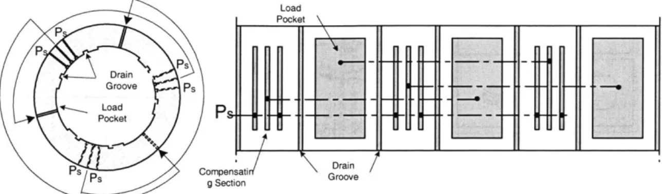
This self-compensating technology can also be applied to hydrostatic journal bearings. Figure 2.3 shows a cross sectional and developed view of a three pocket surface self-com-pensating journal bearing [Geary, 1962].

Load Pocket \ PP\ Ps*-Drain Groove Ps- - -"-- -- * LoadS P s Compensati Groove Pa g Section

Figure 2.3 Cross sectional and developed view of surface self-compensating journal bearing

Another version of the bearing in Figure 2.3 is shown in Figure 2.4 [Stansfield, 1970] It is advantageous to minimize the size of the compensating pockets and maximize load carry-ing pockets. The design of Figure 2.4 is more difficult to design and analyze due to the arrangement of the supply and collecting pockets. The middle section of compensating pocket is at supply pressure and the collecting groove surrounding it is dependent on the eccentricity (location of the shaft). The pressure at the collecting groove then determines the leakage flow out into the drainage grooves. A more deterministic bearing is one where the pressure source surrounds the collecting groove [Slocum 2, 1992]. In this case the outer groove is always at supply pressure and the leakage flow is easier to determine. The journal bearing version of this is shown in Figure 2.5 [Slocum, 1994]. .

Load

Pocket Supply

-tL-Drain Compensating

Groove Pocket

ii'

__ O 690

-7 C

_71

Figure 2.5 Surface self-compensating journal bearing with deterministic compensators [Slocum, 1994] In this version the compensator pocket is removed to the side from the load carrying pock-ets. This is advantageous since the diameter of the bearing is, in most cases, more critical than the length of the bearing.

In [Wasson, 1997, Wasson, 1996] surface self-compensating bearings were introduced that had all the necessary geometry integrated into the shaft. This offers few advantages over the previous designs with geometry in the bushings. First, it makes the precision shrink fit unnecessary and second it can make the manufacturing slightly easier and more cost effi-cient because standard milling tools can be used. Also, in case of cluster spindles, it allows the shafts to be placed closer together by eliminating the need for bushings. Figure 2.6 shows a design where the collector pockets are connected to load pockets by cross drilling through the shaft.

I _{10 11112} 15 11718 _{13 14}1920 4* 5b 7b 2 1 3* 6d 4d 5d 64& 77 4c _{0/ 4} Sc 6b 3C 7

Figure 2.6 Surface self-compensating bearing with cross drilled collectors and load pockets on shaft

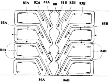
An alternative design that has all the fluid circuitry machined on the surface of the shaft including the connecting passages is shown in Figure 2.7. This will introduce more leak-age flows, but as is shown in later sections, very good performance can still be achieved.The bearing design manufactured in this work is very close to that in Figure 2.7 except that the geometry is on bushing surface. The reasons to have the geometry on bush-ing surface are explained in next section.

83A S2A SIA No 828 S3B

MA

fl)J/(4 / _MB

iT

2.2

Why Bushing?

Having the bearing geometry on bushing surface is advantageous in most cases. The advantages are that the bushing can be made out of good bearing material such as bronze and a standard hardened ground steel shaft can be used without any special manufacturing operations. Manufacturing bushings with geometry on the internal surface only is chal-lenge, which is solved in this work. This makes them more cost effective and interchange-able than the shaft design. Also the balancing becomes an issue when multiple features are machined on the rotating member. A bushing also offers more versatility in terms of linear motion. Having the bearing geometry on the rotary member makes the pressure field unsteady even for fixed journal position due to the local variation of film thickness due to rotation. This can have significant effect at larger eccentricities [Zirkelback, 1998]. This makes the resultant force and force coefficients periodic. In short, the advantages of a bushing are the following:

- More cost effective (with mfg. methods introduced in this work) - More easily replaceable

- More modular

" Better material pairs (unless plain bushing is used with grooved shaft) - Linear motion capability

MODELING

In this chapter two different numerical ways of modeling hydrostatic bearings are described. First, a lumped parameter model based on laminar flow between flat plates is described. Then a finite difference solution method for the Reynold's equation is described briefly and its application to certain features of hydrostatic bearings are dis-cussed. The limitations of both methods are also disdis-cussed. Results from both methods are compared.

3.1 Lumped Parameter Modeling

In the lumped parameter method the bearing is divided into regions where the flow can be approximated by one dimensional fully developed laminar flow between two plates. If the aforementioned conditions are met and gravity is ignored the Navier-Stokes equation for the flow reduces to [Fay, 1994]

2

d u dp

dT - dx (3.1)

By integrating twice and taking into account the non-slip boundary conditions,

u(O) = u(h) = 0, the velocity becomes

u = y(h - y) _(3.2)

By integrating the velocity over the clearance h and multiplying by the width the flow rate is obtained

Q = W (3.3)

By integrating the pressure gradient over the length the hydraulic resistance becomes

R - Ap _ 12pL (3.4)

Q hOw

3.1.1 Validity of the Geometric Assumption

In a general case the assumption of flow between parallel plates is not valid, for example in the case of a journal bearing with non zero eccentricity the surfaces are at an angle. First, the hydraulic resistance for a circumferential flow over land is derived and com-pared to that of Equation 3.4 and then the same is done for axial flow Figure 3.1 describes schematically the situation and the coordinates.

0C 0

Figure 3.1 Circumferential flow over land in displaced journal bearing

h = C( I - Ecos (Oc + (3.5)

Where C is the original clearance. By inserting this into Equation 3.3 the pressure gradient becomes

dp 12pQ 1 (3.6)

dx- W C3 I _Ecos Oc+ ]

By introducing co-ordinate = the hydraulic resistance becomes

R = 2 L 1 d (3.7)

2 1 C _{1 - Ecos (Oc +}

Closed form solution to this integral is long and tedious to find. Figure 3.2 shows the hydraulic resistance of Equation 3.7 divided by the nominal resistance of Equation 3.4, evaluated numerically, as function of eccentricity for ID ratio of 0.1, which is realistic in most cases. Note that this ID ratio is not the same as the bearing ID ratio. It can be noted that even for relatively high eccentricity ratios the difference in hydraulic resistance is very small.

1.05 1.04 1.03 1.02 1.01 1 0.99 0.98 0.97 0 - - - -I - - - - -- - - ---I-- - - --- - - -- - - - --- - - -- - - - -0.2 0.4 0.6 0= 30' 0= ~--- - -0 C _{- - - - -- -}0 0.8 1

Figure 3.2 Ratio between full solution and flat plate approximation in case

of circumferential flow in a journal bearing

a axial flow the pressure gradient is constant and the hydraulic resistance

R 12pL I

Ra lgj 3 1

12!

2

Figure 3.3 shows the hydraulic resistance of Equation 3.8 divided by the nominal resis-tance of Equation 3.4, evaluated numerically, as function of eccentricity for ID ratio of 0.1, which is realistic in most cases. It can be noted that again, even for relatively high eccentricity ratios the difference in hydraulic resistance is very small. It can be concluded that geometric assumption of flow between flat parallel plates is valid for most cases.

600

900

In case of becomes

1.005 1 0.995L .-0.99 -0.985 F - - ---0.98! 0.975 0 0.2 ---- -0.4 0.6 0 _C = 0* --- -- - - 4

---

Figure 3.3 Ratio between full solution and flat plate approximation in case of axial flow in a journal bearing

3.1.2 Example Lumped Parameter Model

Here an example of lumped parameter model implementation for a bearing is presented. The relation of the lumped parameter model to the real geometry is shown in Figure 3.4.

Figure 3.4 Lumped parameter model

300 600 R\,A - - -i-- -i-- -i---i-- -i-- -i-- -i-- -- -R~a R (i))

The resistor symbols represent the hydraulic resistance of the particular flow path it is placed on. The equivalent resistance network is shown in Figure 3.5.

PS" RR(N) R,(1) RJ(2) -R2 R,(N) RI(j) R1(2) Q(2N) - Q(N+1) Q(N+2) R (N) R (1) :tR (2) Pa

Figure 3.5 Equivalent circuit

The resistances R , R1 and Rg of Figure 3.5 are the equivalents of the multiple parallel

resistances R = (3.9) RC I 1 1c2 R = 1 1 1 1 R11I R12 R13 R14 R = S 1 1 1 9 R I+ R I+RI gl g2 g3

There are 3N unknown flow rates, where N is the number of pockets in a bearing. 3N equations are needed to solve for these 3N flow rates. First, N equations are obtained by setting the total pressure drops of the upper loops to zero.

The second set of N equations are obtained by setting the flow rates into each central node to zero (Kirshoff's law)

Q(i) + Q(N + i - 1) - Q(2N+ i) - Q(N + i) = 0 i=1,2,..,N (3.11) The third set of equations is obtained setting the pressure drop across the compensators and pocket land equal to the difference between the supply and atmospheric pressure.

Rc(i)Q(i)+R (i)Q(2N+i) = P P i-1,2,..,N (3.12)

By simultaneously solving the Equations 3.10, 3.11 and 3.12 the unknown flow rates are obtained. Once the flow rates are obtained the pocket pressures are

P(i) = P -Rc(i)Q(i) i=1,2,..,N (3.13)

Once the pressures are known the effective or average pressure on each land can be calcu-lated. This average pressure times the area of each land is the force on each land. These forces can then be divided into components according to whichever co-ordinate system is chosen and then summed to obtain the resulting bearing force. The algorithm for solving the bearing force is the following

e input bearing geometry and displacement

" calculate the hydraulic resistances for each land patch according to Equation 3.4

- Form the system of equations to solve for flow rates (Equations 3.10-3.12) - Solve for the flow rates

* Calculate the pocket pressures according to Equation 3.13 * Form the pressure field in the bearing

3.2 Finite Difference Modeling

The Reynolds equation is the governing equation for fluid flow in thin gaps. The general-ized form of Reynolds equation in x, z coordinate (y is in the direction of film thickness) is [Pinkus, 1961]

ph3 _Jap

+ = 6(U, - _{U2)+(ph) + 12pV}

0

where U1 and U2 are the velocities of the surfaces and Vo is the velocity at which they approach each other. In most cases the other surface is stationary and in a case of steady loading with incompressible lubricant Equation 3.14 reduces to

dh

dx (3.15)

This can be divided into finite differences

h3 _{ij +} I(P i+ -J h3. _ - (i xij 1 Ax

h3 P+1 _( Pi - ,Piij

Az

A schematic grid is shown in Figure 3.6. a (ph3ap) gg,3 (3.14) ah3 a F-(h 3X) a{h3 az( az (3.16) dh 2 2 Ax

4

ax

p

ax)

Pi+ ,j h i+ ,I 2h

n

j

Figure 3.6 Finite difference grid

The clearance can be computed between the pressure points by interpolating between the clearances at the pressure points. Substituting Equations 3.16 into Equation 3.15 and solv-ing for p the following equation is obtained

pi,j = a0 + alpi+ j + a2pi- 1,j + a3Pi,j+1 + a4p _ 1 (3.17)

where ao, aI, a2, a3, a4 are given constants for each point and are

(h