The Distance Effect and the Regionalization of the Trade of Low-Income Countries

HAL Id: halshs-00554326

https://halshs.archives-ouvertes.fr/halshs-00554326

Preprint submitted on 10 Jan 2011

HAL is a multi-disciplinary open access archive for the deposit and dissemination of sci-entific research documents, whether they are pub-lished or not. The documents may come from

L’archive ouverte pluridisciplinaire HAL, est destinée au dépôt et à la diffusion de documents scientifiques de niveau recherche, publiés ou non, émanant des établissements d’enseignement et de

To cite this version:

Céline Carrere, Jaime Melo De, John Wilson. The Distance Effect and the Regionalization of the Trade of Low-Income Countries. 2011. �halshs-00554326�

COMMENTS WELCOME

Document de travail de la série

Etudes et Documents

E 2009. 08

T

T

HHEE

D

D

IISSTTAANNCCEE

E

E

FFFFEECCTTAANNDDTTHHEE

R

R

EEGGIIOONNAALLIIZZAATTIIOONN O OFFTTHHEE

T

T

RRAADDEEOOFF

L

L

OOWW

-

-

I

I

NNCCOOMMEE

C

C

OOUUNNTTRRIIEESS Céline Carrère+ CERDI – CNRS Jaime de Melo♣

University of Geneva and CERDI

John Wilson♦ World Bank

February 2009

+

CERDI (University of Auvergne, France) and CNRS

♣

University of Geneva, CERDI and CEPR

♦

The World Bank

*Thanks to participants at seminars at the World Bank and CERDI. This paper has benefited from support from DFID.

Abstract

The “distance effect” measuring the elasticity of trade flows to distance has been to be rising since the early 1970s in a host of studies based on the gravity model, leading observers to call it the “distance puzzle”. We review the evidence and explanations. Using an extensive data set of 124 countries over the period 1970-2005, we confirm the existence of this puzzle and identify that it only applies to poor countries (the bottom third in per capita income terms in our sample—i.e. the low-income countries according to the World Bank classification, 2006). We show that this group has intensified trade with closer partners and have chosen new partners that are closer than existing partners, leading to a regionalization of their trade at both extensive and intensive margins (regionalization of trade is absent for the other countries). Combining several methods on cross-section and panel estimates of the gravity equation, we estimate that low-income countries exhibit a significant rising distance effect on their trade around 15% between 1970 and 2006 while there is no more distance “puzzle” for trade within richer countries (the top third in per capita income terms in our sample). We dispose of previous explanations of the puzzle, and note that this regionalization could well be a reflection of both increased integration of this group of countries in the world economy or a greater marginalization.

JEL Classification: F10; F40

1

1..IINNTTRROODDUUCCTTIIOONN

There is a widespread perception that the current wave of globalization, much like the first, should have led to the ‘‘death of distance’’. Its

importance for developing countries cannot be underestimated since under a broad range of models, the magnitude of distance effects determines the wage gap with richer countries and the ability to attract footloose industries. In a more popular vein, as argued by Thomas Friedman in The World is Flat (2005), the fall in communication costs which are an integral part of overall transactions costs that are captured by distance, should provide a tremendous opportunity for the poorer

countries to integrate the world economy especially because of their backwardness and the rapid spread of reduction in these costs around the world. With quasi-costless communication, outsourcing will increase and producers in remote developing countries will now be able to supply far-away Northern markets for fashion and other differentiated products with relatively short shelf-lives.

Under this popular interpretation of the “death of distance” scenario, ceteris paribus, the average distance of trade for poorer countries should increase (as lower transport costs would open more distant markets). Yet, no visible increasing trend in the average distance of trade has been

detected in the data over the last thirty years for the poorest. Surprising at it may seem, this is coherent with the high trade costs reported by

Anderson and Van Wincoop (AvW, 2004) in their survey. It is also consistent with the “distance puzzle” which suggests that the burden of distance on trade may have, in fact, been increasing. In terms of the gravity literature used to estimate trade costs, a reduction in trade costs should imply a smaller “distance effect”, i.e. a declining value (in absolute terms) of the elasticity of trade to distance, θ. The challenge then is how to reconcile technology driven reduction in trade costs with a non-shrinking effect of distance in the large literature estimating trade costs from data on bilateral trade.

This puzzle is the subject of this paper. Although we provide several estimates of θ, someone of which are more plausible than previous ones, this is not our main concern (Grossman, 1998 and AvW, 2004 object to its high estimated value).1 _{Instead, we focus on the causes for the persistent} finding that it is increasing with time. We focus on the poorest countries because it is precisely this group of countries that should benefit most

1 _{See the discussion of Grossman’s objection in Anderson and Van Wincoop (2004, p.} 729). Taking into account the quality of infrastructure and the choice of mode of transport (e.g. air, sea) for a cross-section sample of Asian countries, Shepherd and Wilson (2006) obtain a lower estimate θ% = −0.35.

from a flatter world. This focus is also motivated by our earlier work (Brun et al., 2005) where we found that an increasing ‘burden’ of distance was restricted to poor countries and conjectured that they may have been marginalized by the current wave of globalization.

Section 2 reviews the explanations for this finding: composition effects, sample selection, econometric methods and omitted variable bias. This preliminary exploration, in part based on a meta-analysis on 103

published paper (based on the Disdier and Head (2008)’s database), leads us to suggest that the puzzle mainly holds for developing countries. The rest of the paper seeks to check if this is still the case when determinants of distance-sensitive trade costs are brought into the determination of

bilateral trade. Section 3 analyzes the evolution of the average distance of trade, confirming and sharpening the results from the meta-analysis. Over time, the third poorest countries in the sample of 124 countries (i.e. the low-income countries according the World Bank classification of 2006) shift, among existing trade partners, towards physically closer partners. Also, their new trading partners are closer than existing partners. No such pattern is apparent in the data for the remaining countries. These findings confirm a changing role of distance in bilateral trade. In section 4, we revisit the gravity-predicted θ elasticities. To control for as many factors as possible, and to maximize robustness, we rely on cross-section and panel formulations and use several methods to deal with zero trade flows. In all cases, a distance puzzle is revealed for the bottom third (39 countries) in the sample, leading us to conclude that trade has become regionalized for low income countries. Section 5 concludes.

2

2..TTHHEEDDIISSTTAANNCCEEPPUUZZZZLLEEIINNTTHHEEGGRRAAVVIITTYYLLIITTEERRAATTUURREE

2.1. The Rising Distance Effect

While there are several approaches to estimate the impact of transport costs on the volume of trade, the great majority of estimates rely on the popular gravity model which states that the volume of bilateral trade between two countries (i and j) should be proportional to their economic size, proxied by GDP (Y_{i j( )}) and inversely proportional to transport costs, proxied by the distance between partners (D_ij). The numerous studies in the literature deliver an estimate of the elasticity of bilateral trade to distance,

θ

%, which is then used to predict bilateral trade volumes as a function of distance. For example, using the range of estimates in the literature, with

θ

% = −1.4 [ 0.7]− doubling the distance reduces trade by 63%

[42%].2 _{This range is typical of cross-section (sometimes averaged over} 5-year periods) estimates of aggregate trade volumes where trade costs are given by:

( )

( )

1 m M m ij ij ij m t D ρ z γ = =

_∏

(1)

Where, the set z_ijm (m=1,...,M) includes binary dummy variables (usually invariant through time, such as sharing a common border, a common language, etc.) capturing other barriers to trade than distance. These costs enter log-linearly in the “traditional” gravity equation:

(

)

0 1

( )

2

( )

( )

( )

1 ln _ij ln _i ln _j ln _ij M _mln _ijm _ij m M α α Y α Y θ D λ z ε = = + + + + ∑ + (2)

and the distance effect is given by the estimate θ =αρ, with α < being 0 the trade elasticity to trade costs t_ij. As discussed by AvW (2004), and as illustrated in the above typical estimates of θ% , these appear to be

implausibly high. 3 _{This lead AvW to conclude that distance is in fact} capturing other barriers to trade (e.g NTBs, information barriers, and contracting Costs and insecurity) not appropriately controlled for in the set of dummy variablesz_ijm. 4

But the real “puzzle” is that estimates of

θ

% coming from more recent data yield larger estimates. These results imply that distance has exerted a more powerful (negative) effect on the volume of trade in recent times. This is clear from figure 1 below reproduced from a recent meta-analysis of 1,467 elasticity estimates

θ

% compiled from gravity model estimates reported in over 100 published papers (see Disdier and Head, 2008). This figure plots the elasticity estimates against time and fit a kernel smoother through the

2 _{The general formula is:}

(

)

1/ 0 1/ 0

M M = D D θ%

3 _{In the theory-based gravity equation, the elasticity of trade to trade costs depends on the} elasticity of substitution in consumption, σ according to α =

(

σ−1

)

. Since σ has to be estimated separately (as reported by Anderson and Van Wincoop, 5<σ<10), the elasticity of trade to distance will, in fact, depend on the ease with which goods can be substituted across suppliers. As we discuss below, the composition of trade would then appear to matter.

4 _{Based on σ=8, they estimate that the overall border barriers to trade amount to around} 50% .

data (dark line).5 _{From their survey of estimates reported in figure 1 and} from further analysis of the evolution of the estimates through time (see below), Disdier and Head (2008) conclude that the evolution of the distance impact on trade was fairly flat until the 1950s, but has shown a significant increase in the post-1970 data.

Figure 1. The rising Distance Effect in Gravity Models

Source: Disdier and Head (2008, figure 3, p.19).

To give an idea of the orders of magnitude suggested by the meta-analysis summarized in figure 1, distance impedes trade by 37% more since 1990 that it did from 1870 to 1969. This increasing elasticity of trade to distance had already been noticed by Frankel (1997). Earlier, Leamer and

Levinsohn (1995, pp. 1387–88), reviewing the literature on international trade and distance, noted that ‘‘the effect of distance on trade patterns is not diminishing over time. Contrary to popular impression, the world is not getting dramatically smaller.’’ This paradoxical result, now well established, is referred to as the “distance puzzle” or the “missing globalization puzzle” (Coe et al. 2007).

2.2. The Gravity model Set-up

Even though most estimates in figure 1 come from the “traditional” gravity equation in (2), it is now recognized that gravity-based estimates of

changes in trade costs give more intuitive and plausible results when obtained from theory-based gravity models that point out explicitly the channels through which bilateral trade depends on relative trade costs, and indirectly, to distance. To take an example, given trade costs (partly

5 _{The highest R² estimate of each paper is shown with a solid circle, and the lighter blue} lines report the associated lowess smoother estimates.

proxied by distance) will matter less for bilateral trade between New-Zealand and Australia than for bilateral trade between Greece and Switzerland because Australia and New-Zealand are further away from their other trade partners than Greece and Switzerland. A large family of trade models satisfies the conditions necessary to yield a gravity equation at the product level. 6 _{Here is one. Take a one sector economy with a} representative consumer with CES preferences with common

elasticity

σ

among all goods. Impose symmetry of trade costs (tij= tji) and assume that trade costs are proportional to trade (no economies of scale in transport). Then the delivered price includes an ad-valorem equivalent of trade costs (tariffs, NTBs, etc.). With constant returns to scale in transport and marginal cost pricing in transport p_ij = p t_{i ij} = p_i

(

1+

τ

_ij

)

and trade costs enter multiplicatively as in (2). Under these assumptions, outward and inward trade costs P%_i , P%_jare symmetric and the theory-based gravity equation is composed of the system of equations:

1 i j ij ij w i j Y Y t M Y P P σ −     =_{ }    _{ } (3) 1 1 _ij i i j w j t Y P Y P σ σ − −   = _ _  

∑

(4)

where M_ij is the imports of country i from country j , Y_{i j( )} is the GDP of country i (j), Yw is world GDP, tij is bilateral trade costs between i and j, σ >1 is the elasticity of substitution in the CES utility function. According to (3) and (4), bilateral trade flows depend on the relative size of partners and conditionally on relative trade costs where P%_i , P%_j respectively represent the inward and outward multilateral trade resistance.

A more satisfactory formulation of trade would recognize that transaction costs include several components, and that per-unit transport prices may not be equal to transport costs because of market power by transport carriers. Using disaggregated US ocean freight rates over the 1991-2004

6 _{See AvW (2003, 2004). These conditions are: (i) trade separability (i.e. separability in} preferences and technology as in CES technology and utility); (ii) aggregator of varieties are identical and CES across countries; (iii) trade costs are proportional to trade and may include local distribution costs, but these costs do not affect trade flows; (iv) consumer have CES preferences with a common elasticity of substitution σ across commodities. Trade costs do not depend on the quantity of trade, a strong assumption since trade costs are likely to depend on the volume of trade.

period and a cross-section of Latin American freight rates, Hummels et al. (2009) find that ocean-carrier markups are particularly sensitive to tariffs in Latin America and that, jointly with product characteristics, they

explain an order of magnitude more of the variation in shipping prices than distance.7 _{Thus changes in trade policy and in the degree of}

competition in shipping will change the ad-valorem equivalent of trade costs lumped here for convenience under the term ij

τ

. The reduced-form distance-dependent trade cost function would read:

(

)( )

( )

1 1 m M m ij ij ij ij m t

τ

D ρ z γ = = +

∏

(5)

where the ad-valorem equivalent of trade costs includes all border trade costs, depend on product characteristics and on the market characteristics of the transport sector.8 _{In practice, the functional form of trade costs}

ij t is in fact given by (1). Substituting (1) into (3) and (4), the estimated

equation in a cross-section setting becomes:

(

)

( )

( )

( )

(

)

( )

(

)

( )

(

)

( )

(

)

( )

1 ln ln ln ln 1 ln 1 ln 1 ln 1 ln M _m ij w i j ij m ij m i j ij M Y Y Y D z P P

σ

ρ

σ

γ

σ

σ

ε

= = − + + − − + ∑ − + − % + − % + (6)

In this formulation the income coefficient terms are unity, remoteness terms sometimes included in the estimation are derived directly from theory (and called multilateral resistance terms) and the “distance effect” becomes θ =

(

σ −1

)

ρ, the distance elasticity depending on composition effects. Thus a country that would trade mostly homogenous goods with close substitutes would face very small trade costs and the gravity model would not be useful to learn about trade costs in those circumstances.9 Estimates of (6) can be computed from several methods, but most of them are obtained by the inclusion of country fixed-effects which is addition to

7 _{They find that few carriers and high tariffs contribute to the significantly higher} shipping prices facing developing countries and estimate that a 1% reduction in the tariff reduces the shipping price by 1.2% to 2.1% .

8 _{Even though we follow the literature and use the multiplicative form of the trade cost} function, it has been criticized as it implies that the marginal effect of a change in one cost depends on all other costs. Hummels (1999) suggests the alternative additive trade cost

function

(

)( )

1 M m ij ij ij ij m ij m t f τ D ρ γ z =

=_ + _ +

∑

where fij is the freight rate.

9 _{The poor performance of the gravity model for trade among low-income countries is} well-known. Feenstra (2004, chp.5) attributes this poor performance to the non-fulfillment of the critical condition of specialization in different commodities for low-income countries.

producing unbiased estimates, avoids the measurement errors inherent in the use of price indexes. About one quarter of the estimates reported by Disdier and Head (2008) includes these country fixed-effects. As before, a “distance puzzle” obtains when the distance effect, $

θ

, takes larger values when estimated from more recent data as exemplified in figure 1.

Economic and econometric arguments have been advanced to explain the presence of the puzzle. Unfortunately, Disdier and Head (2008) cannot test for each effect separately from the estimates reported in their meta-analysis. For convenience, we categorize these arguments under the headings of sample composition, zeroes in the data and incorporation of multilateral resistance and look for the sensitivity in the estimates of $

θ

to these three set of controls, using the meta-analysis dataset of Disdier and Head (2008).

2.3. Sensitivity of Distance Elasticity estimates in existing empirical literature

Composition Effects. Composition effects appearing through the elasticity of substitution at the product level, have been invoked most. 10 _{Two recent} studies shed some light. Estimating the distance elasticity of bilateral trade for 700 manufactured products in a sample including developing and industrialized countries, Berthelon and Freund (2008) find no evidence that changes in the composition of trade across manufactured

commodities accounts for the distance puzzle (but they give some evidence that for 40% of industries distance became more important). However, compositional changes could take place between broader categories of products. In this vein, Melitz (2007) finds supporting evidence for the argument that there might have been a shift in trade patterns from comparative-advantage-based to intra-industry trade in differentiated products with intra-industry trade mostly among North-North countries that share similar characteristics. Distance has a positive impact on comparative-advantage-based (Ricardian) trade since differences in

endowments /productivities are positively correlated with distance while it has a negative impact for trade in differentiated products. Then, if the share of trade based on comparative advantage decreases (which has certainly been the case if one considers the evolution of the share of agricultural trade in total trade), the negative impact of distance on trade will increase mechanically. In a sample including developed and

developing countries, Melitz (2007) shows that when he introduces the

10 _{Disdier and Head (2008) discuss three channels that will yield different estimates of θ} in theory-based gravity models: differences in σ across products, differences in the response of trade costs to distance across goods ρ and differences in productivity across firms (see also the discussion in Anderson and Van Wincoop, 2004, p.726).

difference in latitude (as a proxy for Ricardian trade), the elasticity estimate of trade to distance falls by half when estimated in several cross-sections over the period 1970 to 1995.11

Composition effects may also be at work through omitted variable bias. Consider for example the impact that the quality and quantity of social and physical infrastructure may have on trade costs that may be captured in the elasticity of trade to distance. Trade costs may be higher in countries with poor-quality institutions (institutions have been found to be

persistent and to change little through relatively long time periods). Then falling communication costs would result in a smaller decrease of trade costs in countries with low-quality social infrastructure. Francois and Manchin (2006) find supporting cross-sectional evidence. Likewise, when they introduce a proxy for contractual enforcement and corruption in the trade cost function, Anderson and Marcouiller (2002) find that the implied tax equivalent of relatively low-quality institutions is 16%. Along similar lines, Aidt and Gassebner (2008) find that autocratic states trade less. While neither finding deals directly with the elasticity of trade to distance, nor with its evolution, they suggest that omitted variable bias could have a systematic impact on the evolution of the elasticity of trade to distance through their impact on trade costs.

Physical infrastructure could also play an important role as first shown by Limao and Venables (2001). Brun et al. (2005) estimated an “augmented” gravity equation incorporating a time-varying indicator of the quality of physical infrastructure. 12 _{The quality of physical infrastructure has also} been brought to light in recent estimates that incorporate indicators of the quality of road infrastructure (Buys et al., 2006 for Africa and Shepherd and Wilson, 2006 for Central Asia).

The characteristics of trade costs could also contribute towards explaining the puzzle. Since international trade involves fixed costs (see the

discussion of evidence in AvW 2004), if technological progress in shipping has been relatively slow in comparison to technical progress in the rest of the economy, then the puzzle could show up in the data through an

increase in transport costs as a fraction of average production costs. This is the interpretation of Estevadeordal et al. (2003) who estimated the

11 _{For reference, when we control for the composition of export by the share of primary} products in total trade, we do not find any effect on the estimated value of θ.

12 _{With this formulation in random-effects estimation over the period 1962-96, Brun et al.} (2005) find falling values through time for

θ

% for trade between countries in the richest tercile in the sample, but they find that the distance puzzle persists for trade between the poorest-tercile countries in the richest tercile. Shepherd and Wilson (2006) also obtain evidence that the quality of infrastructure matters for the volume of bilateral trade.

elasticity of trade to distance for 1913, 1928 and 1938. Brun et al. (2005) and Carrère and Schiff (2005) have also suggested this interpretation: the elasticity of transport costs with respect to distance could increase if the fixed cost component (dwell costs such as port storage costs, loading and unloading costs, time in transit, tariffs on imports, etc.) were falling sufficiently faster than the variable component (e.g. fuel costs, costs of manning and leasing ships). Brun et al. (2005) find that the puzzle holds for developing, but not for developed countries. Finally, Hummels (2001) and Deardorff (2003) suggest that the influence of time on trade is

increasing because of greater use of just-in time production. Then this would show up as rising distance costs.

Handling zeroes in the data. Recent contributions have explored the treatment of zeroes in the data and the handling of the multilateral resistance terms. As argued by Santos Silva and Tenreyro (2006), Martin and Pham (2007) or Eaton and Tamura (1994), ignoring the zero-trade data can severely bias gravity equation estimates. Felbermayr and Kohler (2006) show that standard OLS estimates on the sample of positive traders will yield downwards- biased estimates of the distance coefficient on early data (as zero trade flows due to high trade costs are not taken into account) while more recent estimates (with less zero trade flows) are closer to the “true” values. In other words, if zero trade flows are positively

correlated with large distance (which is clearly the case as discussed below), then ignoring zero trade flows when estimating the gravity equation can generate an “artificial” or spurious distance puzzle.

Relatedly, omitting the multilateral terms when estimating (6) generates a bias in the estimation of θ =

(

σ

−1

)

ρ

since the bilateral distance is

correlated with these multilateral terms that are left in the error term

ε

_ij

(see the discussion in AvW, 2004, page 714).

Finally is the issue of the appropriate functional form for the trade cost function. Coe et al. (2007) find declining distance effects when they specify the gravity equation with an additive error term and estimate it using nonlinear least squares. However, as emphasized by Anderson and Van Wincoop (2004), this is not clear why such estimation would resolve the puzzle. Moreover, using Monte Carlo simulations, Santos Silva and

Tenreyro (2006) find that the nonlinear least squares estimator performs very poorly.

Disdier and Head (2008) started exploring these competing explanations in empirical literature by estimating the following correlates of the

70 79 80 89 90 99 0 1 2 3 m ij m ij i ij m D D D x u e

θ

% =

α

+

α

− +

α

− +

α

− +∑

β

+ + ₍₇₎

where θ% is the jth distance coefficient reported in study i, the D variables _ij

are dummies taking values of 1 when the midyear of the sample used to estimate the jth distance coefficient in study i is in the 70s, 80s and 90s respectively and x_ijmis a set of dummy controls. These dummies control for the presence of developing countries in the sample, for a correction for the zero trade flows, for the use of a country fixed effect, for disaggregated data, etc. (see their table 2 in 44). Finally, the u_i are random effects. In (7), positive estimates for α₁, α₂ and α₃ represents the additional distance effect in, respectively, [1970-1979], [1980-1989] and [1990-1999] compared to pre-1970, once controlled for systematic differences in the attributes of the studies through the x vector.

Their results show that using a sample restricted to developing countries increases significantly the distance elasticity by 0.44 percentage point in the random-effects specification (see their table 2 col. 4 page 44).

Likewise, they find that incorporating zero trade flows in the sample or introducing country fixed effects (i.e. specifying a gravity equation

consistent with theory) increases the distance coefficient by 0.08 and 0.14 percentage points respectively. However, even after controlling for all these aspects of the estimates that could “artificially” create the distance puzzle observed in figure 1, the increasing distance effect after 1970

remains. In sum, the meta-analysis persists in showing a rising estimate of

θ

% across samples, specifications and econometric methods.

To see if these influences vary with time, we extend their exploration by interacting the controls, x_ijm with time dummies, i.e. we estimate: 13

(

)

(

)

(

)

70 79 80 89 90 99 0 1 2 3 70 79 80 89 90 99 1 2 3 ij m m m m m m m ij ij ij m ij i ij m D D D D x D x D x x u e

θ

α

α

α

α

α

α

α

β

− − − − − − = + + + + + + +∑ + + % (8)

We report here results for the three dummy variables that identify the presence of: (i) developing countries; (ii) corrections for the zero trade flows; (iii) controls for the multilateral trade resistance terms suggested by theory i.e. by including either remoteness variables or country fixed

effects.

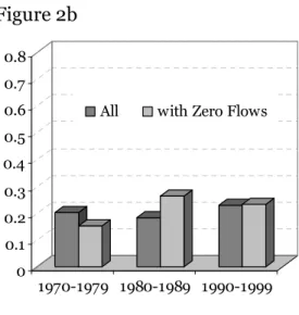
Coefficients of interest are reported in figures 2a-2c. In general, the

coefficient estimates do not vary across time except for studies focusing on developing countries where a very strong distance puzzle is evident after 1970 (each sub-period coefficients is significantly different for the one of the preceding sub-period). These first results would seem to suggest that the most recent developments in the gravity literature on both theoretical and econometric sides — controlling for the zeros trade flows or including multilateral resistance terms —are unlikely to explain the puzzle observed since 1970.

But there are obvious limitations to results obtained from a meta-analysis since the estimates we do have not enough points to really appreciate the evolution of the distance effect within a sample, within a specification or across econometric methods (see Disdier and Head, 2008 for further discussion of other shortcomings).14 _{We return to these issues in section 4} where we explore more systematically the evolution of

θ

% in an integrated framework (i.e. within a sample, gravity model specification or

econometric method).

14 _{For instance, over the 1467 point estimates, only 52 (from 7 different studies) concerns} developing countries.

Figure 2. Distance Puzzle in existing empirical literature Figure 2a Figure 2b 0 0.1 0.2 0.3 0.4 0.5 0.6 0.7 0.8 1970-1979 1980-1989 1990-1999 All

Only Developing Countries

0 0.1 0.2 0.3 0.4 0.5 0.6 0.7 0.8 1970-1979 1980-1989 1990-1999

All with Zero Flows

Figure 2c 0 0.1 0.2 0.3 0.4 0.5 0.6 0.7 0.8 1970-1979 1980-1989 1990-1999

All Country Fixed Effects

Source: authors’ calculations from the Disdier and Head (2008) database.

3. The Regionalization of Trade for Low-income countries

The gravity model with separability in trade costs has two important implications for the evolution of trade. First, it predicts that a relative fall in border-related costs should lead countries to increase the volume of international trade (relative to internal trade). This prediction is largely borne out by the data: since 1980, world production has increased by 75% while international trade has increased by 300% (Berthelon and Freund, 2008). Second, a reduction in all costs related to distance (including better

1 ˆ

α

1 ˆ

α

+

α

ˆ₁m 2 ˆ

α

+

α

ˆ₂m 2 ˆ

α

3 ˆ

α

+

α

ˆ₃m 3 ˆ

α

information about distant markets) should lead countries to increase their volume of trade with distant partners, while on the contrary, if the relative costs associated with distance increase, countries should trade with closer partners. This implication of cost minimization was exploited by Carrère and Schiff (2005) who computed the average distance of trade (ADOT) directly from the bilateral trade data at successive points in time and more recently by Berthelon and Freund (2008) who computed a measure of potential trade (ADOTP_{) predicted by relative country size. The measures} are: =

∑∑

ijt t ij i j wt X ADOT D X (9)

where X_ijtare exports from i to j in t, XWt are world exports in t, and Dij is distance between i and j. The corresponding potential measure is the

gravity-predicted bilateral trade in a frictionless world where the volume of bilateral trade is proportional to the product of the countries GDPs

(denotedY_{( )i t}): ; =

∑∑

=

∑∑

=

∑∑

p ijt it jt P p p t p ij wt ijt i j wt i j i j wt X Y Y ADOT D X X X Y (10)

This measure will change only as a result of changes in the dispersion of incomes around the world and it will be maximal if all countries have the same size. So, in a gravity world, a higher potential trade for a group of countries simply means less dispersion in economic size in that group. Feenstra (2004, chp. 5) reports results showing that this measure of potential trade fits the data quite well for developed countries but less for developing countries.

Then, if gravity is an adequate description of the volume of bilateral trade, the ratio of potential to actual trade is a measure of trade costs. Since it is suggested by the gravity model we call this ratio the average distance ratio (ADR):

/ P

t t t

ADR =ADOT ADOT (11)

The values of these ratios are reported for our sample of 124 countries over the period 1970-2006.15 _{To iron out fluctuations, each point is a 5-year}

15 _{The sample includes all countries except microstates and ex-FSU countries giving us a} balanced sample (see the list of countries in appendix A1, table A1.1). But using the complete sample of 190 coutries does not change the results presented here and in the rest of the paper (results available upon request). Nominal bilateral trade flows (in US$,

average. Because of the preliminary results suggesting that low-income countries are different, we also report averages for the richest and poorest tercile of countries (each tercile has 39 observations). To ease the reading, we set ADRt to 1 in for the period 1970-1974. It can be seen that the ADR ratio is quite stable fluctuating around the value of 1 for the whole sample, even though the small decline could be taken to suggest that barriers to trade have been increasing in relative terms, leading countries to shift trading patterns towards closer partners.

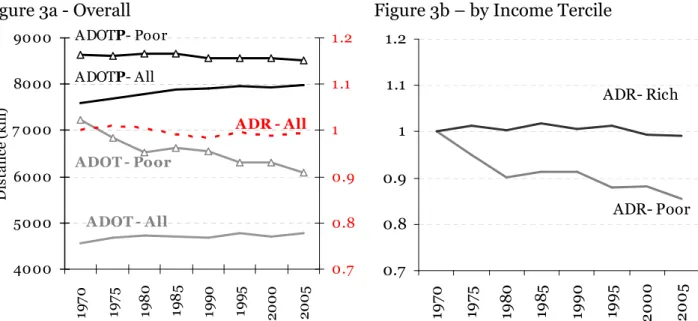
As suggested by the systematically higher estimates of the elasticity of trade to distance for developing countries in the meta-analysis, we also report separately the potential and actual distance of trade for the poorest third (39 countries) in the 124 in the sample with all countries in the sample. 16 _{By selecting all trade of the poorest countries rather than trade} with only the remaining (85) countries, we are addressing directly the issue of whether their trade is becoming more regionalized, regardless of the partners.

Figure 3 shows a higher potential trade for the poorest countries, reflecting larger dispersion in incomes for this group. More interesting is the large fall in the average distance of trade for this group implying that poor countries have shifted their trade towards geographically closer partners. For this group the average distance of imports fell by more than 15% from 7200 kms in 1970-1974 to 6000 in 2005-2006.

c.i.f), are taken from UN-COMTRADE (via WITS), divided by the US deflator. We use import data as it is well-recognized that they are more accurately reported by the customs authorities. For developing country, we use mirror estimates, i.e. export data reported by partner countries. GDP and population are taken from the World’s Bank World

Development Indicators 2008. Distance measures and dummy variables indicating whether the two countries are contiguous, share a common language, or have had a common colonizer are from the Centre d’Etudes et de Prospectives et d’Informations Internationales (CEPII). The simple distances are calculated following the great circle formula, which uses latitudes and longitudes of the most important city (in terms of population).

16 _{The list of countries is given in appendix A1, table A1.1. The computation of terciles was} carried out by splitting the country in three groups on the 1970-2006 average. We then checked if the classification would have changed if we had used beginning or end-of-period GDP figures. Concerning for instance the poorest tercile, compared to the list reported in table A1.1, China and Sri Lanka would have been included in this group at the beginning of the period (instead of Haiti and Zimbabwe) while Ivory Cost Only would have been included in this group (instead of Pakistan) at the end. Note that the poorest tercile matches perfectly the low-income country group as defined by the World Bank in 2006.

Figure 3. Average distance and Indirect Trade Cost Measures for 124 countries, 1970-2006

Figure 3a - Overall Figure 3b – by Income Tercile

4000 5000 6000 7 000 8000 9000 19 7 0 19 7 5 19 8 0 19 8 5 19 9 0 19 9 5 2 0 0 0 2 0 0 5 D is ta n ce ( k m ) 0.7 0.8 0.9 1 1 .1 1 .2 ADOTP- All ADOT - All ADR - All ADOTP- Poor ADOT - Poor 0.7 0.8 0.9 1 1.1 1.2 19 7 0 19 7 5 19 8 0 19 8 5 19 9 0 19 9 5 2 0 0 0 2 0 0 5 ADR- Rich ADR- Poor

Note: 5-years periods over 1970-2004 and a 2-years period 2005-2006 Source: authors’ calculations on data from UN-COMTRADE and WITS.

This changing pattern is reflected in diverging paths of the ADR ratios for the whole sample and for the lowest tercile. If the gravity model is an adequate of representation of the determinants of trade, then we get in figure 3a confirmation of the meta-analysis results of figure 2a: the costs of barriers to trade for the poorest countries have gone up in relative terms with a fall of 15% in the average distance of trade over the sample period.

Why did poor countries switch to closer trade partners? 17 _{In this simple} setting, the only two possibilities are changing weights of existing trading partners, or changing trading partners. First, it could be that close trading partners (e.g. China and India in Asia) grew fast. This would result in the observed regionalization of trade for the poorest tercile. If so, we should then also observe a decrease in the average potential distance because of the increasing GDP weights for the close partners. However, figure 3a indicates that the potential distance of trade barely increases, so this effect cannot be a major factor.

17 _{To illustrate this point, we report in appendix A4 the 3 main import suppliers of each of} the 39 poorest countries of the sample with their trade share and distance, for 1970-1975 and 2005-2006

Note: 5-years periods over 1970-2004 and a 2-years period 2005-2006

Source: authors’ calculations on data from UN-COMTRADE and WITS

Poorest Tercile (39) Richest Tercile (39)

6 0 0 0 6 5 0 0 7 0 0 0 7 5 0 0 8 0 0 0 8 5 0 0 1970 1975 1980 1985 1990 1995 2000 2005

Average Distance (km, unweight ed)

M=0 M>1 6 0 0 0 6 5 0 0 7 0 0 0 7 5 0 0 8 0 0 0 8 5 0 0 1970 1975 1980 1985 1990 1995 2000 2005

Av erage Dist ance (km, unweighted)

M=0 M>1

Poorest Tercile (39) Richest Tercile (39)

0 % 1 0 % 2 0 % 3 0 % 4 0 % 5 0 % 6 0 % 7 0 % 8 0 % 9 0 % 1 0 0 % 1970 1975 1980 1985 1990 1995 2000 2005

Number of observat ions (balanced=4,7 97 )

M>1 M=0 0 % 1 0 % 2 0 % 3 0 % 4 0 % 5 0 % 6 0 % 7 0 % 8 0 % 9 0 % 1 0 0 % 1970 1975 1980 1985 1990 1995 2000 2005

Number of observ ations (balanced=4,7 97 )

M>1 M=0

The other possibility is a change in the composition of trading partners. Indeed, as shown in figure 4, over the sample period, the number of zero trade flows is quite stable until 1990, around 45% for the poorest tercile and 15% for the richest tercile. 18 _{Then the number of zero trade flows} decreases sharply and fell by half. In contrast to the richest tercile, the average distance of zero trade flows for the poorest tercile is consistently higher than for positive trade flows, but the gaps narrow in later years.

The effect of this expansion of trade and its implication for the average distance of trade is shown in figure 5 for the poorest tercile. The figure disaggregates the ADOT for the lowest tercile into the two components: (i) “traditional”, i.e. existing trade partners with already positive trade flows in 1970-1974 (intensive margin); (ii) “new” trade partners with positive trade flows since 1975 (extensive margin). We also report the weights of each trading partner (or each margin) in total trade.

Figure 5: Average Trade Distance of Poorest countries with Traditional and New Trade Partners

0% 1 0% 20% 30% 40% 50% 19 7 5 19 8 0 19 8 5 19 9 0 19 9 5 2 0 0 0 2 0 0 5 R a ti o ( N ew P a rt n er s/ T o ta l) 3000 4000 5000 6000 7 000 8000 A D O T 3 9 P o o rs ( k m s)

Nber obs. Import Value

A DOT - Trad. Partners A DOT - New Partners

Two patterns are evident: first the regionalization of trade is partly reflecting the closer distance of the “new” partners that are significantly closer than the existing partners and they have an increasing weight in the

18 _{We observe in the mid-1980s a slight increase in the number of zero trade flows} compared to preceding years mainly for the poorest country’ trade. This slowdown in trade growth around the mid-1980s is also visible in Felbermayr and Kohler (2006, figures 3a and 3b based on Rose’s database) and in Helpman, Melitz and Rubinstein (2008, figures 1 and 2, based on Feenstra’s database). As these new (and temporary) zero trade flows also concern geographically close partners, this results in a decrease of the unweighted average distance of zero trade flows during the 1980s.

total value of imports. Hence, part of the puzzle is along the extensive margin. Second, within the existing “traditional” group, the poorest countries have shifted towards geographically closer partners.19 _{In the} absence of data on the product composition of new trade partners, it is difficult to know what leads developing countries to choose closer trading partners since it could reflect a change in product composition as new products are initially shipped to close partners. In any case, it is clear from figure 5 that the regionalization of trade is also generated by trade

redistribution within the intensive margin. 20

The conclusion from this inspection of the raw data is that the poorest countries have shifted trade towards physically closer trading partners which would be expected from gravity theory if the relative trade costs with physically closer partners fell more than trade costs with further-away partners. This could be the case if the closer partners are those who reduced most their barriers to trade. In addition, even though on average partners with zero trade are further away than partners with positive trade, when extending trade to new partners, the poorest countries have selected those countries that are closest. Both patterns are consistent with a minimization of trade costs in a formulation in which distance matters. These patterns could also have resulted from the proliferation of regional trade agreements among the poorer countries.

The next section explores if this increasing elasticity of trade to distance only applies for the poorer countries in the sample after controlling for some of the factors that could alter distance-sensitive trade costs.

4

4..TTHHEEPPEERRSSIISSTTEENNTTRRIISSIINNGGDDIISSTTAANNCCEEEEFFFFEECCTTFFOORRLLOOWW--IINNCCOOMMEE

C

COOUUNNTTRRIIEESS

If the gravity model is an adequate representation of bilateral trade, one should obtain increasing values of the elasticity of trade to distance (the “distance effect”),

θ

% , over time in the gravity model, but only for

developing countries. This is indeed what comes out of the alternative estimates below: repeated cross-sections (each cross-section representing a 5 years average) as in the vast majority of cases reported in the

19 _{We checked that the patterns described are robust when we drop alternatively India} (included as reporter in the group of the 39 poorest countries and dominates other countries in terms of trade value) and China (included in the 123 partner countries) from the sample. Results of figure 5 are unchanged (available upon request).

20 _{In a cross-section estimation of trade costs on the number of products exported by a} country, Allen and Shepherd (2007) find robust and quantitatively significant positive estimates of the number of product varieties to a battery of trade costs with lower trade costs leading to increases in product varieties.

analysis; and panel estimates in which the estimated coefficient of distance is allowed to vary over time. The panel formulation is more suitable to incorporate time-dependent trade costs identified in (5) which we do when we build a time-series index of the quality of infrastructure. The panel estimates also allow for a better control for omitted variables by using country-pair specific effects. Hence, under panel estimation, omitted bilateral effects are no longer captured by the distance coefficient. On the other hand, because the number of zero trade flows is important for most of the sample period (especially for the poorest tercile), it is useful to explore several methods for controlling for zero values. This is better done in cross-section than in panel. We start with cross-section estimates, then turn to the panel estimates.

4.1 Cross-section Estimates

We follow the by-now standard approach and estimate:

(

)

0 ln

( )

ln

( )

ln =α +α +α +θ +

∑

λ m +ν ij m ij m ij i j D z ij M (12)

where α_i and α_j are the importer and exporter fixed effects that capture the multilateral resistance variables, and all other variables that are country specific and that will appear in the panel estimates: GDPs’, multilateral term indexes and indices of the quality of infrastructure.21

Results are reported in table 1 for the first and last periods under different estimation methods to account for the zero trade flows in the data with the evolution of the estimated distance elasticity reported in figures 6 and 7.22 Column (1) serves as a reference and reports OLS estimates in which the zero trade flows are considered as missing variables (this corresponds to the majority of estimates reported in the meta-analysis). Column (2) reports the results from the standard solution in the literature using

(

)

ln 1+M_ij instead of ln

(

M_ij

)

as the dependent variable (see e.g. Frankel, 1997). This increases the mean value of exports by one unit without affecting its variance and, with this correction, country-pair with zero trade flows are represented by a zero value of the dependent variable (ln 1

(

+M_ij

)

). However, the OLS estimator does not take into account the

21 _{In this sample with low-income countries it is preferable to use OLS rather than the} systems approach used by AvW to avoid the measurement error associated with the multilateral resistance variables. The log-linear approximation proposed by Baier and Bergstrand (2009) will be used in the panel estimates reported below.

censorship of the dependent variable. Column (3) reports the results from the Eaton and Tamura (ET, 1994) tobit with ln

(

a+M_ij

)

as dependant variable. Under the ET estimator, instead of arbitrarily imposing a= , the 1 value of the a parameter is endogenously determined and the dependent variable will be censored at the value ln a

( )

.23 _{Finally column (4) reports} the results from the Poisson Pseudo Maximum Likelihood (PPML) estimator proposed by Santos Silva and Tenreyro (2006) to deal with heteroskedasticity in log-linear gravity models.24 _{Because of the} controversy about the way to deal with zeros in the data, it is useful to compare the estimates under the two estimators.25 _{Note however, that if} we control for the censorship bias due to the relatively large number of zeros in the data, we do not decompose the distance effect into within-intensive and extensive margins as proposed by Helpman, Melitz and Rubinstein (2008). While extending the estimation to explore this issue is interesting, and was already explored partly using the descriptive statistics in preceding section, a credible improvement would require a plausible identification variable for the first step for this sample over 1970-2006.26

23 _{We also ran a Tobit estimator on ln 1}

(

)

ij M

+ which produced similar results to those

obtained with the Eaton-Tamura estimator (see appendix A3, table A3.1). For the (ET) Tobit estimator with country dummies, we did not use the complicated transformation for a fixed effects Tobit developed by Honoré (1992) but a “simple” pooled Tobit as developed in Wooldridge (2002, pages 540-542). See also Arellano and Honoré (2001, section 7). 24 _{We fit conditional fixed effects PPML (see details in Arellano and Honoré, 2001, section} 5).

25 _{The PPML estimator handles the inconsistency introduced by log-linearization model} in the presence of heteroskedasticity, but it is not clear that it is a better estimator to handle the presence of zeroes in trade data. Using Monte-Carlo simulations, Santos Silva and Tenreyro show that that the PPML estimated of (12) with M_ijas dependent variable produce estimates with the lowest bias for different patterns of heteroskedasticity (compared to OLS on ln 1

(

+M_ij

)

and a tobit on ln

(

a+M_ij

)

, see their table 5 page 30). However, Martin and Pham (2008) pointed out that Silva and Tenreyro used a data-generating-process for their Monte Carlo analysis which is a fundamentally different data generating process from that underlying the zero values in models of Eaton and Tamura (1994) or Helpman, Melitz and Rubinstein (2008). When correcting the data-generating process, Martin and Pham (2008) find that the Eaton and Tamura (1994) Tobit estimates have a lower bias than those obtained with the PPML estimator.

26 _{To do so would require a two-stage equation estimation procedure with a selection} equation for the decision to trade across partners (identifying the extensive margin) followed by a trade flow equation in the second stage (identifying the intensive margin). Helpman, Melitz and Rubinstein (2008) use “regulation costs of firm entry” as

identification variable for their 1986 cross-section regression. However, yearly (or five-year average data) necessary for a credible identification strategy, are not available.

Table 1. Barriers to Trade: Cross-section results

Methods OLS OLS ET- Tobit PPML OLS OLS ET- Tobit PPML

dependent var. ln(M) ln(1+M) ln(a+M) M ln(M) ln(1+M) ln(a+M) M

(1) (2) (3) (4) (5) (6) (7) (8) lnDij -1.066*** -1.115*** -1.231*** -0.668*** -1.429*** -1.336*** -1.325*** -0.710*** (0.0352) (0.034) (0.034) (0.000) (0.0303) (0.038) (0.029) (0.000) Common Border 0.898*** 0.326* 0.244* 0.367*** 0.821*** 0.613*** 0.584*** 0.555*** (0.142) (0.178) (0.132) (0.000) (0.146) (0.188) (0.115) (0.000) Common Language 0.702*** 1.001*** 1.201*** 0.328*** 0.967*** 1.112*** 0.967*** 0.203*** (0.0638) (0.058) (0.063) (0.000) (0.0585) (0.064) (0.053) (0.000) Colonial links 1.315*** 1.401*** 1.329*** 0.589*** 0.639*** 0.663*** 0.695*** 0.00188*** (0.114) (0.134) (0.161) (0.000) (0.109) (0.142) (0.141) (0.000) Nber Obs. 10,403 15,252 15,252 15,252 13,384 15,252 15,252 15,252

% of zero Trade flows 0% 32% 32% 32% 0% 12% 12% 12%

R² or pseudo-R² 0.698 0.745 0.743 0.877 0.799 0.817 0.910 0.905

2005 1970

Standard errors in parentheses, *** p<0.01, ** p<0.05, * p<0.1. Fixed country effects are not reported.

Source: authors’ calculations

Several patterns stand out in table 1. First, as expected, the dummies have the usual signs and usual significance levels. There are however some changes in the coefficient values over the sample period reflecting

expectations from a globalizing world. The value of the common language coefficient falls drastically through time: based on columns (4) and (8) (the PPML estimation), sharing a common language increases trade by 39% in 1970-74 but only by 22% in 2005-06. Colonial links also become far less important quantitatively over the period, increasing trade by around 80% in 1970-74 but only 0.2% in 2005-06.

The estimates of θ are high, but well in the range of values reported in figure 1. Importantly, the PPML elasticity estimate is much lower and more plausible than the values obtained with the other estimators.Santos Silva and Tenreyro (2006) explain this systematic difference in the

estimated value between the OLS and the PPML estimators by the heteroskedasticity rather than by the censorship bias. 27 _{The explanatory} power of all the models reported in Table 1 is quite high and increase over time, suggesting that the gravity model is a better representation of

bilateral trade in later years.28 _{One reason for this better fit would be}

27 _{See the discussion in Santos Silva and Tenreyro (2006). Since the coefficient on the} PPML represents the marginal estimate of a change in distance on bilateral trade, the coefficients also represent trade elasticities to distance. Note that the OLS on ln(1+M)) and ET tobit estimates give very close results on this sample.

28 _{R² are not directly comparable to pseudo-R² as the number of observations is not} always the same and more importantly, the R² are based on sums of squares whereas the peudo-R² are based on ratios of log-likelihoods.

better data, especially for developing countries. Another, would be a

change in the trade structure of developing countries as development leads to a shift towards trade in differentiated rather than homogenous

products, hence towards a situation closer to that depicted by the gravity model (see e.g. the evidence in Feenstra, 2004 and Evenett and Keller, 2002).

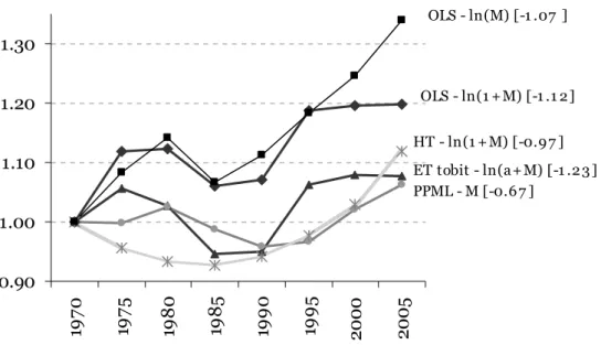
Figure 6. Cross-Section Estimates of the Elasticity of Trade to Distance θ

0.90 1.00 1.10 1.20 1.30 19 7 0 19 7 5 19 8 0 19 8 5 19 9 0 19 9 5 2 0 0 0 2 0 0 5 OLS - ln(1 + M) [-1 .1 2 ] ET tobit - ln(a+ M) [-1 .2 3 ] PPML - M [-0.6 7 ] HT - ln(1 + M) [-0.9 7 ] OLS - ln(M) [-1 .07 ]

Note: 5-years periods over 1970-2004 and a 2-years period 2005-2006 Corresponding Trade elasticity to distance in 1970 reported into brackets. Source: authors’ calculations

Finally, the time-plot of the estimates of θ in figure 6 (with all distance coefficients normalized to unity on the first sub-period 1970-1974)

confirms the existence of a puzzle. The puzzle is robust across estimators. Two conclusions come out of this comparison. First, the strong distance puzzle obtained in literature is partly due to the fact that, until recently at least, zero values were not handled by OLS estimates with no specific correction for the censorship of the sample. However, even after controlling for the zero trade flows, the distance puzzle remains highly significant. Second, the range of estimates obtained across the different methods produces a rather narrow range of estimates with the burden of distance on trade significantly higher at the end of the period in the range [+6.3%; +7.6%]. Taken together, these results confirm that the distance puzzle holds up to the scrutiny of typical econometric problems.

To check whether the increasing values of θ is attributable to the presence of developing countries, we re-estimate the (12) by introducing dummy variables for the richest and poorest terciles, i.e. we regress:

(

)

0 ln

( )

ln

( )

ln

( )

ln . m ij ij m ij m I ij i j D D ij z ij M =α +α +α +θ +θ I +

∑

λ +ν (13)

with alternatively the dummy Iijequals to 1 if:

- i or j belongs to the third poorest countries in the sample; - i and j belongs to the third richest countries.

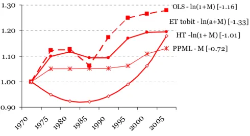
Figure 7. Cross-Section Estimates of θ by Tercile Figure 7a. 39 poorest’ trade with all countries

0.90 1.00 1.10 1.20 1.30 1970 1975 1980 1985 1990 1995 ₂₀00 2005 OLS - ln(1 +M) [-1 .1 6] ET tobit - ln(a+M) [-1.33] PPML - M [-0.72] HT -ln(1+ M) [-1.01]

Figure 7b. Within 39 richest countries

0.90 1.00 1.10 1.20 1.30 1970 1975 1980 1985 1990 1995 2000 2005 PPML - M [-0.65] OLS - ln(1+M) [-0.98] ET tobit - ln(a+M) [-1.14] HT -ln(1+ M) [-0.89]

Note: 5-years periods over 1970-2004 and a 2-years period 2005-2006, Corresponding Trade elasticity to distance in 1970 reported into brackets.

The results of this estimation are displayed in figures 7. It is clear that the results are due to the presence of developing countries in the sample since the estimates of θ in figure 7b show no more significant distance effect increase for the richest tercile and this is robust across estimators (except for the OLS estimates which are biased). By contrast the estimate of θ increases in the range [+13%; +19%] for the poorest tercile. Taken at face value, these estimates suggest that a doubling of distance would reduce poorest country’s trade by 60% in 1970-74 and by 67% in 2005-2006 according to the ET tobit results (and respectively 39% and 43% in the PPML regressions).

4.2. Panel Estimates

Panel estimates allow the introduction of trade costs that vary through time and that are lumped together in (5) under the term

τ

_ij assumed to capture the ad-valorem equivalent of trade costs such as tariffs,

communication and other transaction costs. In the absence of time-series data on border measures and other transaction costs, we follow earlier contributions (e.g. Limao and Venables , 2001 and Brun et al., 2005) and construct a time-series index of the quality of infrastructure for each country which becomes the new proxy for the bilateral transport costs, tijt. The augmented distance-dependent trade cost function becomes:29

( )

1

(

)

2

(

)

3

ijt ij it jt

t = D ρ K ρ K ρ (14)

As constructed (see appendix A2), larger values for Ki(j)t indicate a better infrastructure. 30_{Again, the choice of functional form matters. If the cost} function was additive with the infrastructure component independent of distance, the elasticity of transport costs to distance could increase if the fixed cost component were falling sufficiently faster than the variable component.31

29 _{Since bilateral specific effects capture the time-invariant characteristics of bilateral} trade, the trade cost function no longer includes the colonial, language and border dummy variables. Nor does it include fuel costs due to the year dummies.

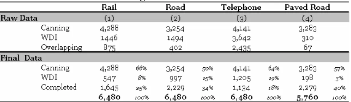
30 _{To compute the infrastructure index, we use data from the telecommunication sector} (number of main telephone lines per 1000 workers), and the transportation sector (the length of the road and railway network —in km. per sq. km. of land area) and an index of the quality in the service of transport (the share of paved roads in total roads) from Canning (1998) and World Development Indicators Database (see details in appendix A2).

This trade cost function is introduced in (3) and (4) with country-pair fixed effects (FE) to capture the time-invariant characteristics of bilateral trade. Since these effects were not captured by the FE in the cross-section

estimates, the panel estimates offer another robustness check on the earlier results although this is at the cost of imposing a trend specification for the evolution of distance. In particular, the country-pair fixed effects control for the North-South differences that Melitz (2007) found to reduce the estimate of θ by half over the period 1970-1995.32 _{Furthermore, the} panel specification allows for some asymmetry in the gravity equation since the bilateral specific effect on imports of i from j can be different from the corresponding bilateral effect of imports of j from i (see equation below).33 _{Finally, year effects are included to capture all year shocks}

common to all country pairs such as variations in the cost of fuel (arguably a main factor affecting the marginal cost of transport).

To account for the variation of the multilateral resistance terms through time, we adopt the linear approximation proposed by Baier and Bergstrand (2009) to obtain unbiased and consistent reduced-form estimates (see the details in appendix A5). The estimated equation is:

(

)

( )

( )

( )

(

)

( )

(

)

(

)

1 2 3 4 5 6 ln ln ln ln ln ln ln ln ijt it jt ij it jt it jt ijt t ij M Y Y D K K MR MR λ β β β β ε

λ

θ

β

β

= + + − + + + + + + (15) where ln( ) , ln( ) kt kt it ik jt kj k wt k wt Y Y MR D MR D Y Y     =  = 



∑

 

∑

 are the multilateral resistance

or

“remoteness” variables, 34 _and t

λ is a vector of year dummies, λ_ij the bilateral fixed effects (with λ_ij ≠λ_ji) and

ε

_ijt the error term.35 _{A quadratic} time trend:

32 _{Melitz (2007) regresses in OLS an equation very close to our OLS on ln(M) on 158} countries over 1970-1995 (five-years sub-periods). He obtained an increase in distance coefficient of around +18.8% while we find, over the same period +18.3% (using a random effect Hausman-Taylor specification on ln(M), see below). Once he controlled for North-South distance, Melitz obtained an increase in distance of around +8%, while with our corresponding random effect HT specification on ln(M) over 1970-1995 yields an estimated increase of +4%.

33 _{Helpman, Melitz and Rubinstein (2008) motivate their model allowing for zero and} asymmetric trade flows on data indicating asymmetry in trade flows over 1970-1997. 34 _{Virtually the same results are obtained with the ad-hoc remoteness variable which uses} the logs of the GDP weighted average distance rather than the GDP weighted average of the logs of the bilateral distance.

35 _{Note that the random effect specification implies}

ijt ij ijt

ε =µ +υ with µ_ij is a specific bilateral random effect, and υijt is the idiosyncratic error term with the usual properties.

2 1 2. 3. θ ≡ _∂ ∂ _ =θ +θ +θ   ijt ij ijt ij M D t t M D (16)

is introduced in(15) to detect any significant evolution of ˆθ. Because estimation in panel with bilateral fixed effects (FE), we also use a bilateral random effects (RE) estimator to obtain an estimate of the impact of distance on trade. Because the GDPs (Y_{i j t( )} ) and infrastructure indices (K_{i j t( )} ) are correlated with the bilateral random effects (µ_ij), we correct for this endogeneity using the Hausman-Taylor (1981) instrumental variables method.36

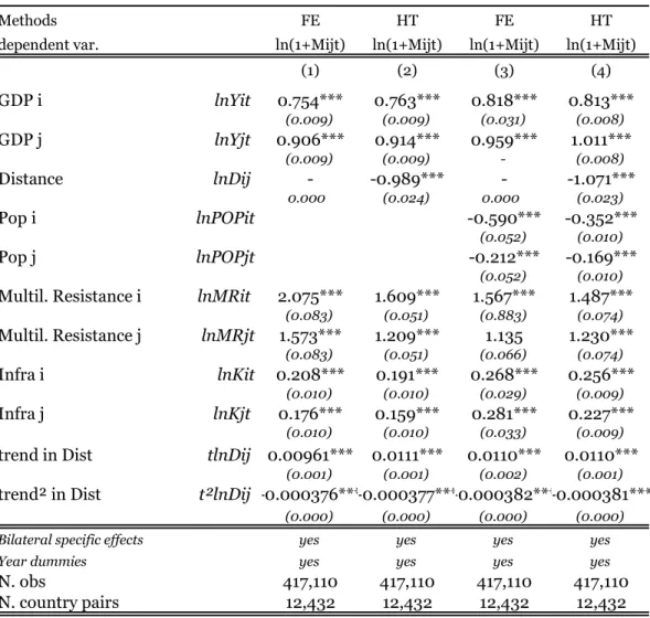
Results are reported in table 2. Note first that the FE and RE estimates in cols. 1 and 2 are very close indicating that endogeneity issues have been handled adequately (this is the case for all the variants). Signs and magnitude of coefficients are plausible. As suggested by the theory, the elasticity of trade with respect to income is significant and close to unity. The negative coefficients for the population variables confirm that larger countries are more self-sufficient (or that poorer countries trade less). It could also reflect that for large countries, the costs of trading with

themselves rather than with others is relatively less. The multilateral resistance variables also have the expected positive sign. Thus given the absolute distance between i and j, the further country i is far from its trade partners, the more country i will trade with j. As expected, an

improvement in the quality of infrastructure increases significantly the volume of trade. One could also interpret these positive coefficients in the broader sense of proxies for the quality of social infrastructure (physical infrastructure is largely a public good that will be underprovided in countries with poor social infrastructure). The distance coefficient in the HT specification is close to unity when taking into account the zero trade flows (ln(1+Mt)).

The estimated trend from column (4) is reported in figure 6. It is slightly higher than the trend estimated with the ET tobit or the PPML (+11% vs. 7.6% and 6.3% respectively). Using the same approach as in (13), we also estimate the trend for the richest and poorest terciles and report the results in figure 7. Again, the results are quite close to those obtained by the repeated cross-section estimations. While it could be argued that not accounting for the censorship of zeroes in the panel estimates might make

36 _{We carry out a pretest estimator based on Hausman (1978) (see Baltagi, Bresson and} Pirotte (2003) to choose between the fixed effects, random effects, and HT estimators. The test statistics lead us to choose the HT estimator. See Brun et al. (2005) appendix B for the construction of instruments and the choice of estimator.

a difference, given the close values across estimators in the cross-section results in table 1, it is unlikely that not accounting for truncation would have significantly changed the results here.

Table 2. Panel estimations

Methods FE HT FE HT

dependent var. ln(1+Mijt) ln(1+Mijt) ln(1+Mijt) ln(1+Mijt)

(1) (2) (3) (4) GDP i lnYit 0.754*** 0.763*** 0.818*** 0.813*** (0.009) (0.009) (0.031) (0.008) GDP j lnYjt 0.906*** 0.914*** 0.959*** 1.011*** (0.009) (0.009) - (0.008) Distance lnDij - -0.989*** - -1.071*** 0.000 (0.024) 0.000 (0.023) Pop i lnPOPit -0.590*** -0.352*** (0.052) (0.010) Pop j lnPOPjt -0.212*** -0.169*** (0.052) (0.010)

Multil. Resistance i lnMRit 2.075*** 1.609*** 1.567*** 1.487***

(0.083) (0.051) (0.883) (0.074) Multil. Resistance j lnMRjt 1.573*** 1.209*** 1.135 1.230*** (0.083) (0.051) (0.066) (0.074) Infra i lnKit 0.208*** 0.191*** 0.268*** 0.256*** (0.010) (0.010) (0.029) (0.009) Infra j lnKjt 0.176*** 0.159*** 0.281*** 0.227*** (0.010) (0.010) (0.033) (0.009)

trend in Dist tlnDij 0.00961*** 0.0111*** 0.0110*** 0.0110***

(0.001) (0.001) (0.002) (0.001)

trend² in Dist t²lnDij -0.000376***-0.000377***-0.000382***-0.000381***

(0.000) (0.000) (0.000) (0.000)

Bilateral specific effects yes yes yes yes

Year dummies yes yes yes yes

417,110 417,110 417,110 417,110 12,432 12,432 12,432 12,432 N. obs

N. country pairs

Robust standard errors in parentheses *** p<0.01, ** p<0.05, * p<0.1

We carried out two further robustness tests on the trend estimates (not reported here). First, we checked the sensitivity of estimates to imposing unitary elasticities on the GDPs. The results are unchanged. Second, we controlled for composition effects that preoccupied Melitz (2007) using the share of primary exports to control for the composition of exports