HAL Id: hal-02942469
https://hal.archives-ouvertes.fr/hal-02942469
Submitted on 17 Sep 2020
HAL is a multi-disciplinary open access
archive for the deposit and dissemination of
sci-entific research documents, whether they are
pub-lished or not. The documents may come from
teaching and research institutions in France or
abroad, or from public or private research centers.
L’archive ouverte pluridisciplinaire HAL, est
destinée au dépôt et à la diffusion de documents
scientifiques de niveau recherche, publiés ou non,
émanant des établissements d’enseignement et de
recherche français ou étrangers, des laboratoires
publics ou privés.
Distributed under a Creative Commons Attribution| 4.0 International License
middle atmosphere observed during Titan’s late
northern spring to early summer
S. Vinatier, Christophe Mathé, B. Bézard, J. Vatant D’ollone, S. Lebonnois,
C. Dauphin, F. M. Flasar, R. K. Achterberg, B. Seignovert, M. Sylvestre, et al.
To cite this version:
S. Vinatier, Christophe Mathé, B. Bézard, J. Vatant D’ollone, S. Lebonnois, et al.. Temperature
and chemical species distributions in the middle atmosphere observed during Titan’s late northern
spring to early summer. Astronomy and Astrophysics - A&A, EDP Sciences, 2020, 641, A116 (33p.).
�10.1051/0004-6361/202038411�. �hal-02942469�
Astronomy
&
Astrophysics
https://doi.org/10.1051/0004-6361/202038411 © S. Vinatier et al. 2020
Temperature and chemical species distributions in the middle
atmosphere observed during Titan’s late northern spring to
early summer
?
S. Vinatier
1, C. Mathé
1,2, B. Bézard
1, J. Vatant d’Ollone
3,4, S. Lebonnois
3, C. Dauphin
5, F. M. Flasar
6,
R. K. Achterberg
6, B. Seignovert
7, M. Sylvestre
8, N. A. Teanby
8, N. Gorius
6, A. Mamoutkine
9,
E. Guandique
10, and D. E. Jennings
6(Affiliations can be found after the references) Received 13 May 2020 / Accepted 19 June 2020
ABSTRACT
We present a study of the seasonal evolution of Titan’s thermal field and distributions of haze, C2H2, C2H4, C2H6, CH3C2H, C3H8,
C4H2, C6H6, HCN, and HC3N from March 2015 (Ls=66◦) to September 2017 (Ls=93◦) (i.e., from the last third of northern spring to
early summer). We analyzed thermal emission of Titan’s atmosphere acquired by the Cassini Composite Infrared Spectrometer with limb and nadir geometry to retrieve the stratospheric and mesospheric temperature and mixing ratios pole-to-pole meridional cross sections from 5 mbar to 50 µbar (120–650 km). The southern stratopause varied in a complex way and showed a global temperature increase from 2015 to 2017 at high-southern latitudes. Stratospheric southern polar temperatures, which were observed to be as low as 120 K in early 2015 due to the polar night, showed a 30 K increase (at 0.5 mbar) from March 2015 to May 2017 due to adiabatic heating in the subsiding branch of the global overturning circulation. All photochemical compounds were enriched at the south pole by this subsidence. Polar cross sections of these enhanced species, which are good tracers of the global dynamics, highlighted changes in the structure of the southern polar vortex. These high enhancements combined with the unusually low temperatures (<120 K) of the deep stratosphere resulted in condensation at the south pole between 0.1 and 0.03 mbar (240–280 km) of HCN, HC3N, C6H6
and possibly C4H2 in March 2015 (Ls=66◦). These molecules were observed to condense deeper with increasing distance from the
south pole. At high-northern latitudes, stratospheric enrichments remaining from the winter were observed below 300 km between 2015 and May 2017 (Ls=90◦) for all chemical compounds and up to September 2017 (Ls=93◦) for C2H2, C2H4, CH3C2H, C3H8, and
C4H2. In September 2017, these local enhancements were less pronounced than earlier for C2H2, C4H2, CH3C2H, HC3N, and HCN,
and were no longer observed for C2H6and C6H6, which suggests a change in the northern polar dynamics near the summer solstice.
These enhancements observed during the entire spring may be due to confinement of this enriched air by a small remaining winter circulation cell that persisted in the low stratosphere up to the northern summer solstice, according to predictions of the Institut Pierre Simon Laplace Titan Global Climate Model (IPSL Titan GCM). In the mesosphere we derived a depleted layer in C2H2, HCN, and
C2H6 from the north pole to mid-southern latitudes, while C4H2, C3H4, C2H4, and HC3N seem to have been enriched in the same
region. In the deep stratosphere, all molecules except C2H4were depleted due to their condensation sink located deeper than 5 mbar
outside the southern polar vortex. HCN, C4H2, and CH3C2H volume mixing ratio cross section contours showed steep slopes near
the mid-latitudes or close to the equator, which can be explained by upwelling air in this region. Upwelling is also supported by the cross section of the C2H4(the only molecule not condensing among those studied here) volume mixing ratio observed in the northern
hemisphere. We derived the zonal wind velocity up to mesospheric levels from the retrieved thermal field. We show that zonal winds were faster and more confined around the south pole in 2015 (Ls=67−72◦) than later. In 2016, the polar zonal wind speed decreased
while the fastest winds had migrated toward low-southern latitudes.
Key words. planets and satellites: individual: Titan – planets and satellites: atmospheres – planets and satellites: composition – methods: data analysis – radiative transfer – infrared: planetary systems
1. Introduction
Because of the 26.7◦ obliquity of Saturn, its system including
Titan experiences strong seasonal changes. The Cassini mission arrived at the Saturn system on July 1, 2004 (Ls=293◦), during
the middle of Saturn’s northern winter and ended on September 15, 2017 (Ls=93◦), a few months after the northern summer
sol-stice. Titan Global Climate Models (GCMs) predict that during northern winter the global dynamics of Titan’s middle atmo-sphere (from the deep stratoatmo-sphere to the mesoatmo-sphere) consists
?The data are only available at the CDS via anonymous ftp to
cdsarc.u-strasbg.fr (130.79.128.5) or via http://cdsarc. u-strasbg.fr/viz-bin/cat/J/A+A/641/A116
of one global circulation cell upwelling at high-southern lati-tudes and subsiding at high-northern latilati-tudes (Newman et al. 2011; Lebonnois et al. 2012, 2014; Lora et al. 2015; Vatant d’Ollone et al. 2018). Impacts of this predicted dynamics were observed on the temperature field derived from the Cassini Composite Infrared Spectrometer (CIRS) observations of Titan’s atmosphere thermal emission. The highest mesospheric temper-atures, which were derived above the winter pole (Flasar et al. 2005;Achterberg et al. 2008,2011;Coustenis et al. 2010;Mathé et al. 2020; Teanby et al. 2007, 2008; Vinatier et al. 2007, 2010a), resulted from adiabatic heating of the subsiding branch of the pole-to-pole circulation cell. Additionally, this polar subsi-dence transported the air enriched in photochemical compounds A116, page 1 of33
produced at higher altitude levels towards the deep stratosphere where some molecules such as HC3N or C4H2were observed to
be enhanced by several orders of magnitude compared to their values outside the winter polar vortex (Coustenis et al. 2007; Mathé et al. 2020;Teanby et al. 2007,2008;Vinatier et al. 2007, 2010a). Around the northern spring equinox, which occurred on August 11, 2009 (Ls=0◦), GCM predict changes of this
dynami-cal pattern with a two-year transition period involving a two-cell circulation regime with air upwelling at low latitudes and sub-sidence at both poles.Achterberg et al.(2011), who derived the seasonal evolution of the temperature field from July 2004 to December 2012 (Lsfrom 293◦to 4◦) using CIRS spectra, showed
that the subsiding branch at the north pole had already weak-ened before the northern spring equinox. In the early southern fall, the first southern polar molecular enhancements, derived from CIRS limb spectra analysis, were observed in June 2011 (Ls=22.7◦) at altitudes higher than 400 km (Teanby et al. 2012;
Vinatier et al. 2015), showing that the southern polar subsidence had already settled at that date. From the combined interpretation of the meridional cross sections of temperature and haze, C2H2,
HCN, and C2H6 volume mixing ratios (VMRs) derived from
CIRS limb observations acquired between July 2009 (Ls=359◦)
and May 2013 (Ls=45◦),Vinatier et al.(2015) showed that the
global dynamics had entirely reversed within about two years after the northern spring equinox.
One of the most striking events of the southern fall was the unexpected 30 K cooling of the polar stratopause and meso-sphere between June 2011 and February 2012 (Ls=22.7◦−30.6◦)
(Teanby et al. 2017;Vinatier et al. 2015) at least partly explained by the increased efficiency of radiative cooling by the strongly enhanced photochemical species and the decreasing solar flux, while the subsidence was strengthening the adiabatic heating (Teanby et al. 2017). The southern polar enrichment contin-ued to strengthen after this date, reaching its maximum in March 2015 (Ls=65.8◦; Mathé et al. 2020), while the polar
stratospheric temperature continually decreased before increas-ing again around September 2015 (Ls=72◦) (Teanby et al. 2017).
The southern molecular polar enrichment combined with the low stratospheric temperatures were at the origin of the devel-opment of a large stratospheric polar cloud first observed in May 2012 by the Cassini Imager SubSystem (ISS;West et al. 2016). Several ice signatures were detected inside this cloud at differ-ent altitudes: HCN ice (de Kok et al. 2014; Le Mouélic et al. 2018), C6H6 ice (Vinatier et al. 2018), the “haystack” cloud at
220 cm−1 (Jennings et al. 2012, 2015) and the High Altitude
South Polar (HASP) cloud possibly containing co-condensed C6H6:HCN ice (Anderson et al. 2018). Seasonal evolution of
this cloud was monitored using the Cassini Visible and Infrared Mapping Spectrometer (VIMS) byLe Mouélic et al.(2018).
At high-northern latitudes, Teanby et al. (2019) and Coustenis et al. (2020) showed from analysis of CIRS obser-vations acquired in nadir geometry that the northern winter photochemical species enhancements resulting from their trans-port by subsidence remained during the entire northern spring. They assumed constant-with-height VMR as vertical informa-tion is poor for most of molecules with this observing mode, which mostly probe the 1–10 mbar range. We show in our study that molecular VMR vertical profiles in this region varied greatly with altitude and that the northern spring polar enrichment was in fact confined to the mid-stratosphere (0.1–1 mbar pressure range).
Titan’s deep stratosphere, at 15 mbar, also underwent sea-sonal variations at both poles with a temperature decrease of 25 K at 70◦S between January 2007 and June 2016 and a
temperature increase of 7 K at the north pole in the same period (Sylvestre et al. 2020). The south pole enriched air was also observed at the 15 mbar level at latitudes higher than 70◦S in
late 2012 (Sylvestre et al. 2018) with continuous increase of the VMR with time. Indeed, near 70◦S, VMR of C4H2 and C2N2
were 30 and 40 times higher in 2016 than in 2009, respectively, while CH3C2H was enriched by a factor of 10 in the same period.
Our goal in this paper is to study in detail the seasonal evolu-tion of the thermal field and the VMR meridional cross secevolu-tions of nine molecules and aerosols, from one pole to another and from 5 mbar up to 50 µbar (120–650 km), to determine how the remaining northern polar enrichment resulting from the previous winter vanished at the approach of the northern summer solstice and how the southern polar vortex evolved during the second part of the southern fall. We aim to interpret these observations in terms of seasonal changes of the dynamics through compar-ison with prediction of the Institut Pierre Simon Laplace Titan Global Climate Model (IPSL Titan GCM).
We have analyzed CIRS mid-infrared spectra acquired at the limb of Titan from January 2015 to September 2017 (the end of the Cassini mission) to retrieve temperatures; VMRs of C2H2,
C2H4, C2H6, CH3C2H, C3H8, C4H2, C6H6, HCN, and HC3N;
haze extinction; and derived zonal wind in the stratosphere and the mesosphere. We have extended as much as possible our retrievals to provide new hints on dynamical and chemical pro-cesses occurring in the mesosphere. This study extends the work of Vinatier et al. (2015), which focused on the temperature field and the C2H2, HCN, C2H6, and aerosol VMRs around the
northern spring equinox, from July 2009 to May 2013, in the 5– 10−3 mbar (120–500 km). Between 2012 and 2015, the Cassini
orbit inclination was too high to probe both poles in limb geom-etry viewing, and it is why we focus here on limb data analysis between 2015 and the end of the Cassini mission in September 2017.
Section 2describes the CIRS limb observations sequences used in this study. The retrieval method and the inferred temper-ature field and photochemical species VMR cross sections are presented in Sects.3and4, respectively. Results are discussed in Sect.5.
2. Observations
Our study is based on the analysis of thermal emission of Titan’s limb acquired by the Cassini/CIRS spectrometer. CIRS was a Fourier transform spectrometer acquiring spectra in the far-infrared (from 10 to 600 cm−1) with a 3.9-mrad FWHM circular
detector on Focal Plane 1 (FP1) and in the mid-infrared through two linear arrays each composed of ten 0.273-mrad field-of-view detectors on Focal Plane 3 (FP3, from 570 to 1125 cm−1) and
Focal Plane 4 (FP4, from 1050 to 1495 cm−1). A detailed
descrip-tion of the CIRS instrument and an overview of the different observing modes are given inKunde et al.(1996),Flasar et al. (2004) and Nixon et al. (2019). FP3 and FP4 were specially designed to probe the vertical structure of Titan’s atmosphere, while these linear detector arrays were positioned parallel to a Titan radius when Cassini was at a distance from Titan’s surface of 100 000–200 000 km, so that each detector had a vertical res-olution of about one scale height (∼40 km). During a single limb sequence (above a given latitude and longitude), each FP3 and FP4 detector array pointed successively at two positions in the atmosphere: the deep atmosphere with the ten-detector line-of-sight altitudes spanning from the surface to about 350 km and then the upper stratosphere and mesosphere with lines of sight spanning the ∼300–700 km region. Each FP3 and FP4 detector
array therefore pointed successively at two altitude ranges with an overlap of about ∼70 km in the 300–400 km altitude region. Combining the two pointing positions of FP3 and FP4 arrays allowed us to probe the atmosphere between 100 to 650 km. As 30 to 50 spectra were usually acquired during a single position by each of the ten detectors of FP3 and FP4 at very similar alti-tudes, we averaged them per detector (and therefore for a given altitude level) to increase the signal-to-noise ratio (S/N) of the spectra used in our retrievals. In order to derive the temper-ature and photochemical compound global spatial and vertical distributions, we used dedicated FP3 and FP4 CIRS limb obser-vation sequences, in which an entire hemisphere was scanned while Cassini was approaching or leaving Titan during a given flyby. Such observations had an apodized spectral resolution of 15.5 cm−1. More details on this observation type, called
mid-infrared limb maps (MIRLMBMAP), are given inNixon et al. (2019).
Data used here are extracted from the “global calibration” version (Jennings et al. 2017) archived in the NASA Planetary Data System. We analyzed 11 MIRLMBMAP sequences and combined those acquired within two consecutive Titan flybys, usually within a two-month time period, to derive pole-to-pole spatial distributions of the temperature and photochemical com-pound VMRs. When these sequences did not cover the polar regions, we also analyzed spectra acquired in a nadir viewing geometry mode at 3-cm−1 spectral resolution to complete the
spatial distributions derived from limb observations. We then determined global spatial distributions for seven time slots from March 2015 to September 2017. Details of the observations used here are given in TablesB.1andB.2.
3. Retrieval of the temperature and photochemical compound mixing ratio profiles
The observed molecular rovibrational emission bands intensities depend on both temperature and molecular VMRs. The contin-uum emission is due to the haze extinction and the collision-induced absorption of N2-N2, N2-CH4, CH4-CH4, and N2-H2. In
order to infer both temperature and chemical compound VMR vertical profiles, we proceeded in several steps. In the first step we retrieved simultaneously, from the FP4 limb spectra, the temperature profile by fitting the ν4-CH4 band in the 1200–
1330 cm−1 spectral range and the haze extinction profile from
the fit of the continuum in the 1080–1120 cm−1spectral range.
In the second step these profiles were incorporated in our atmo-spheric model to derive the molecular VMR profiles from the fit of their emission bands in FP3 limb spectra. For both steps we determined the vertical profiles using an inversion algorithm based on the fit of the observed limb spectra using a line-by-line radiative transfer code. The inversion algorithm and the spec-troscopic files used here are described inVinatier et al.(2010b, 2015). We additionally utilized here the propane pseudo-line list of Sung et al.(2013) to reproduce the C3H8 ν7, ν21, ν20, and
ν7 emission bands centered at 869, 922, 1054, and 1158 cm−1,
respectively. We used the spectral dependence of the aerosol extinction coefficient from Vinatier et al. (2012) to reproduce the continuum of all selected limb spectra. As in our previous studies (Vinatier et al. 2007, 2010a,2015), we had to apply a shift on the CIRS database nominal line-of-sight altitudes of our selected limb spectra to reproduce the P- and Q-branches of the ν4-CH4band of the deepest limb spectra, which display the
high-est S/Ns. In previous analyses we applied this shift to the lines of sight of all averaged limb spectra acquired in a given limb; at the beginning of the Cassini mission the relative pointing of the two
positions of the FP4 detector array in a given limb sequence was accurate so that radiances of detectors in the overlapping alti-tude region were consistent within the Noise Equivalent Spectral Radiance (Teanby et al. 2007). However, for the limb sequences used here, we found a discontinuity in the vertical profile of the limb integrated radiance in the overlapping zone of the two pointing positions of the FP4 array. To ensure a continuity of the integrated radiance profile, we first determined the shift to apply to the lowest pointing position where limb spectra have the highest S/Ns. After applying this shift to the lines of sight of the deepest position of the FP4 array, we then determined what shift to apply to the pointing altitudes of the upper pointing position to get a continuity of the entire radiance vertical profile (including both pointing positions). A similar method was also used byMathé et al.(2020) for all CIRS limb spectra acquired at a 0.5-cm−1 spectral resolution. The applied shifts are given
in Table B.1. We applied the same shifts to the limb spectra acquired by the FP3 because FP4 and FP3 spectra were acquired simultaneously.
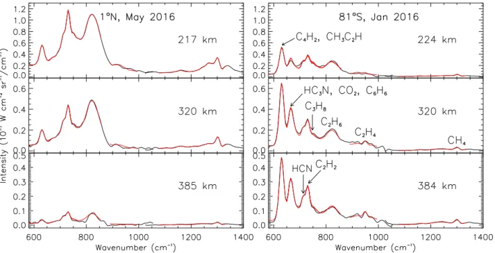
After constraining the temperature profile, we incorporated it in our atmospheric model to reproduce the radiance of the molecular emission bands in the FP3 spectral region. At 15.5 cm−1 resolution, several molecular emission bands are
mixed (i.e., for C4H2 and CH3C2H or HC3N, CO2, and C6H6;
see Fig. 1). The only well-separated emission bands are those of C2H6 and C2H4. The haze thermal emission also contributes
to the continuum in the entire FP3 spectral range. In order to properly reproduce the continuum, we retrieved the haze opti-cal depth profile simultaneously with C4H2and CH3C2H mixing
ratio profiles from the 595–660 cm−1spectral range in which the
595–610 cm−1 region is free of molecular emission bands. We
then utilized this retrieved haze optical depth profile to model the continuum radiance in the entire FP3 spectral range.
As HC3N, CO2, and C6H6emission bands are mixed, and as
the CO2 VMR does not vary with latitude or season (Vinatier
et al. 2015;Mathé et al. 2020), we fixed the CO2VMR profile to
the one derived byVinatier et al.(2015) at 0◦N in May 2012. The
HC3N and C6H6mixing ratio profiles were retrieved from the fit
of the 660–678 cm−1spectral range. C2H2, HCN, and C3H8were
retrieved simultaneously from the 705–750 cm−1 range, C2H6
was retrieved from the 800–850 cm−1 range, and C
2H4 from
the 900–986 cm−1region (excluding the 952.5–958 cm−1region
because of an instrumental noise spike there). Examples of fits of these spectral ranges are displayed in Fig.1.
Even though the detected emission in the mesosphere can-not entirely be considered in local thermodynamic equilibrium (LTE; Feofilov et al. 2016), we chose to retrieve thermal and VMR profiles at altitudes as high as possible, assuming LTE everywhere in order to highlight upper levels in which infor-mation is available, postponing a more appropriate retrieval including non-LTE effects for a later dedicated study.
4. Results
4.1. Temperature field
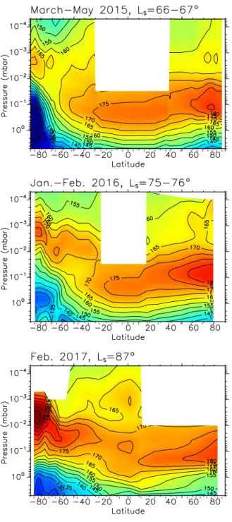
The temperature meridional cross sections retrieved from Ls=66◦ (March 2015) to Ls=93◦ (September 2017) are
dis-played in Fig.2(with a pressure y-axis) and in Fig.C.1(polar representation with an altitude vertical axis calculated assuming hydrostatic equilibrium). The polar cross section of March-May 2015 is the only one that extends across both poles (see Fig.C.1). In both figures, regions without information (in white) corre-spond either to a lack of data, poor S/Ns, or altitude levels not
Fig. 1.Example of CIRS limb spectra acquired at 1◦N in July 2016 (left panel, black line) and 81◦S in January 2016 (right panel, black line) at
three different tangent heights. They are compared with the best fit spectra (in red). These spectra can be compared with those of Fig.1ofMathé et al.(2020, their Figs. 1 and 2) acquired at similar location, altitude, and date at higher spectral resolution. The band centered at 630 cm−1includes
C4H2and CH3C2H emission; the band centered at 673 cm−1includes HC3N, CO2, and C6H6. HCN, C2H2, and C3H8emission bands are centered
respectively at 713, 730, and 748 cm−1. C2H6, C2H4, and CH4bands are centered at 815, 950, and 1300 cm−1, respectively. An overlap between FP3
and FP4 spectra occurs in the 1000–1050 cm−1spectral range.
probed by nadir observations. Temperature profiles derived from limb observations were usually constrained in the 120–650 km range (∼5 mbar to 5 × 10⁻⁵ mbar), while nadir observations
probed the 120–400 km region (∼5 mbar to 10−2mbar) except
at high-southern latitudes where they probed up to 550 km (∼5 ×10⁻⁴mbar) because of the very steep vertical thermal
gra-dient there. The retrieved thermal profiles including their error bars are available in supplementary material and will be posted on the Virtual European Solar and Planetary Access (VESPA) portal1. Error bars are usually smaller than 1 K below the
stratopause and can reach a few kelvins at mesospheric levels. Error bars include uncertainties due to spectral noise and the ±2 km uncertainty on the determined vertical shift.
4.1.1. High-southern latitudes
The most striking seasonal changes in temperature between Ls=66◦and Ls=93◦were observed in the southern hemisphere
at latitudes higher than 30◦S, where the stratopause altitude
varied with latitude in a complex way. The southern polar stratopause reached its highest temperature close to the south pole (Figs.2 andC.1), its temperature increased by 10 K from March to September 2015 (Ls=66◦−72◦) and by 22 K from May 2016 to February 2017 (Ls=78◦−87◦) to reach its highest value
of 207 K. For the time period studied here, the altitude of the stratopause was globally decreasing towards mid-latitudes.
At deeper levels, the polar stratosphere was at its cold-est in March and September 2015 (Ls=66◦ and Ls=72◦) with
temperatures lower than 120 K observed below the 0.06 mbar pressure level (260 km altitude) in March and the 0.2 mbar
1 Vertical profiles are accessible on the VESPA portal: (http://
vespa.obspm.fr/planetary/data/). Fits of the observed spectra
are available on request to S. Vinatier.
level (∼200 km) in September. As the southern autumn was progressing, these low temperatures were observed to propagate deeper.
4.1.2. Mid-southern latitudes
Interestingly, the 30◦S latitude seemed to be a transition in the
structure of the thermal field from September 2015 (Ls=72◦)
to May 2016 (Ls=78◦): on the low-latitude side, the stratopause
was located deeper (∼0.2 mbar, 250 km) than toward higher lat-itudes (at 40◦S, it was located at 3 × 10⁻³ mbar, 450 km). It
resulted in a double 173 K stratopause structure at 30◦S (Figs.2
andC.1). On both sides of 30◦S, the stratopause remained at
sim-ilar pressure levels until May 2016, while in February 2017 the two local temperature maxima seemed to have merged into a sin-gle one around 3 × 10⁻²mbar (340 km). This new structure was
observed until the southern winter solstice in May 2017, the last date for which we have limb observations at this latitude. 4.1.3. Northern hemisphere
Thermal profiles in the northern hemisphere showed moderate changes during the second half of the northern spring. Altitude of the stratopause remained the same (∼300 km, 0.1 mbar) at all latitudes from Ls=67◦ to Ls=93◦ (May 2015 to September
2017) with similar temperature (about 175–180 K) everywhere except at latitudes higher than 70◦N, where the stratopause was
typically 5 K warmer than at lower latitudes. After the north-ern summer solstice (for Ls=93◦), at high-northern latitudes the
stratosphere was ∼2 K colder and the stratopause 5 K colder than at Ls=76◦ (February 2016), while an opposite trend was
observed in the mesosphere, which was ∼5 K warmer (in the 0.2−1 × 10⁻² mbar region) after the northern summer solstice
Fig. 2.Temperature meridional cross sections from March 2015 to September 2017. Contours are given every 5 K from 110 to 205 K; the color scale is the same for all plots. In the equatorial region, pressures of 1, 0.1, 0.01, 10−3, and 10−4mbar roughly correspond to altitudes of 200, 300,
400, 500, and 600 km, respectively. Regions without information are represented in white; they correspond to missing data or pressure levels not probed by nadir observations. Red ticks on the x-axis give latitudes of observations used to retrieved the global map.
4.1.4. Possible correlation between mesospheric temperature and insolation
We infer a local temperature maximum in the mesosphere around 500 km (10−3 mbar) during Titan’s daytime. For instance, a
165 K temperature local maximum was observed at this pressure level at high-northern latitudes in May 2015, at a solar zenith angle (SZA) of 63–90◦, and February 2016 (17:00 local time,
SZA = 60–66◦), at mid-northern latitudes and the equator in June
2016 (∼15:00 local time, SZA = 30–60◦), and around the equator
and at low-southern latitudes in February 2017 (12:30 local time, SZA = 19–45◦). In contrast, it seems that the coldest mesospheric
temperatures were observed during the night; for instance, tem-peratures about 5 K higher were found at the end of the day above 10−3 mbar at mid-northern latitudes in November 2015 (local
time ∼17:50, SZA = 68–85◦) than in the middle of the night in
May 2015 (local time ∼01:30, SZA of 95–113◦). In the
south-ern hemisphere the lowest mesospheric temperatures were also observed during the night; for instance, in February 2017, the 10−4-mbar level temperature was found to increase from 162 K
at 09:22 local time at 50◦S (SZA = 82◦) to 167 K at 12:48 at 2◦N
(SZA = 26◦).
In the northern hemisphere, which was experiencing spring, we also inferred that the more illuminated high-northern lat-itudes showed higher mesospheric temperatures. For instance, in September 2017 the mid-northern latitude mesosphere (from Equator to 40◦N, SZA = 106−153◦, 21:30-22:47 local time) was
∼5 K colder at 10−4 mbar than the constantly insolated
high-northern latitude (local time ∼20:30, SZA = 72–85◦). A similar
mesospheric temperature trend was also observed in May 2015 as the colder mid-northern latitude mesosphere was in the night (∼01:30 local time, SZA = 90-113◦) and the high-northern
latitude mesosphere was insolated (SZA = 60-86◦).
Mesospheric temperatures seem to be correlated with solar insolation even if adiabatic heating (respectively cooling) due to air subsidence (respectively upwelling) can also impact the mesospheric temperatures. This possible correlation, which can only be detectable in the mesosphere where the radiative time constant is about a few Titan hours (Bézard et al. 2018), was not observed deeper at the stratopause and stratospheric levels, consistently with the predicted radiative time constant greater than one Titan day there (Bézard et al. 2018).
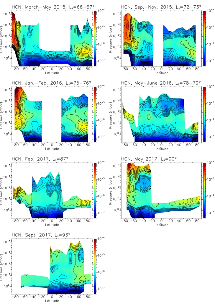
4.2. Molecular gas mixing ratio meridional cross sections Outside the southern polar region C2H2, HCN (Figs. 3, A.2,
andC.1middle and bottom panel) and C2H6(Figs.A.1andC.2
bottom panel) are the molecules whose VMR could be derived up to a few 10−4mbar (500-600 km). C4H2and CH3C2H VMR
(Figs. A.3, A.4 and C.2) were generally determined up to a few 10−3 mbar (450–500 km). C3H8 and C2H4 mixing ratios
(Figs.A.5,A.8,C.3andC.4) were usually inferred up to 10−2–
10−3mbar (400–450 km) and HC3N and C6H6(Figs.A.6,A.7,
andC.3) were mostly detected at high latitudes up to 600 km at the south pole, while in the mid- and low-latitude regions, their VMRs (usually lower than 10−9) should be considered as upper
limits. Retrieved mixing ratio profiles including their error bars are available in the supplementary material and will be posted on the Virtual European Solar and Planetary Access (VESPA) portal2. Determination of the error bars follows the methodology
described byVinatier et al.(2010a). They include the uncertainty
2 Vertical profiles are accessible on the VESPA portal: http://
vespa.obspm.fr/planetary/data/). Fits of the observed spectra
are available on demand to S. Vinatier.
on the retrieved thermal profiles, the ±2 km uncertainty on the vertical shift, and the spectral noise, all summed quadratically at each pressure level.
Before looking in detail at the spatial distributions of each molecule, we first depict the main common global spatial and temporal trends of the inferred VMR:
– Most molecules were strongly enriched at high-southern latitudes inside the polar vortex because of the subsidence of the global circulation cell that settled in 2012 (Teanby et al. 2012; Vinatier et al. 2015) and transported enriched air from higher lev-els toward the deep stratosphere. Additionally, this polar air was isolated from the air at mid-southern latitudes by strong zonal winds (Achterberg et al. 2011,2018; West et al. 2016) forming the polar vortex (see also Sect. 5.5). At a given date, all polar VMR distributions (except those of C2H6 and C3H8 that have
limited vertical gradients and therefore show limited enhance-ment by subsidence) showed very steep meridional gradients at high-southern latitudes, tracing the polar vortex barrier (Teanby et al. 2008). Depending on the molecules, polar enhancements were the greatest in 2015 and in January 2016. In March 2015 the molecules showing the steepest concentration meridional gradi-ents across the polar vortex boundary were C2H4, C3H4, C6H6,
HC3N, and HCN, which varied from a factor of 10 for HCN
to three orders of magnitude for HC3N and C6H6. In
Septem-ber 2015, this polar enriched region had a wider latitudinal extension than in March 2015 and January 2016, and displayed stronger enrichments than in May 2017, suggesting changes in the horizontal structure of the polar vortex over this period.
– In May 2017, at high-southern latitudes (between 30◦S
and 60◦S) and at altitudes higher than 500 km (10−3 mbar),
C2H2, C2H6, C4H2, CH3C2H, and HCN were more abundant
than earlier in the season, while their polar enhancements in the 10−1–10−3mbar region were less pronounced, suggesting some
changes in the global circulation occurring close to the southern winter solstice.
– In the deep stratosphere, typically below the 1 mbar level, at mid- and low latitudes all molecular VMRs (except for C2H4
which does not condense) decreased with depth as the main sink of these molecules is condensation, usually occurring below the 10 mbar level (∼100 km). Some molecules, like HCN, C4H2,
and CH3C2H, show steep slopes in the contours of constant
mixing ratio at low- or mid-latitudes (see, e.g., Fig. A.4 in May-June 2016 or Fig. A.2 in Sept.-Nov. 2015), which sug-gests that upwelling was transporting deeper air (depleted due to condensation) to upper levels in the stratosphere.
– Mesospheric depletions in C2H2, HCN, and C2H6
(Figs. 3,A.1, A.2,C.1 and C.2), which are the molecules for which we can derive information at the highest levels, have been observed since September-November 2015 (Ls=72−73◦). This
depletion seems to have been initiated at high-northern latitudes in May 2015 (Ls=67◦) and has extended down to mid-southern
latitudes in September 2015 (Ls=72◦).
– Although at high-northern latitudes the upwelling branch of the global circulation cell has been in place since probably mid-2011 (Vinatier et al. 2015), a region located at latitudes higher than 60◦N and altitudes between 200 and 300 km (Figs.3
to4 and Figs.C.1toC.4) remained enriched in photochemical compounds (including haze) until the northern summer solstice, with a tendency to vanish after this date. Most of these molecular enrichments were located at the stratopause level. This suggests that the stratopause could be a sort of stagnancy region with limited mixing or that the northern winter residual circulation cell (which keeps some of the winter polar enriched air in the deep stratosphere up to the stratopause) was still present over the
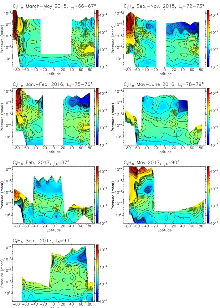
Fig. 3.C2H2volume mixing ratio meridional cross sections from March 2015 to September 2017. Regions without information are represented in
white; they correspond to missing data or pressure levels not probed by nadir observations. Red ticks on the x-axis give latitudes of observations used to retrieved the global map.
Fig. 4.Haze mass mixing ratio meridional cross sections from March 2015 to September 2017, determined from the haze extinction meridional cross sections displayed in Fig.A.9. Regions without information are represented in white; they correspond to missing data or pressure levels not probed by nadir observations.
entire spring, as predicted by the IPSL Titan GCM, albeit limited to the deep stratosphere for all compounds (see Sect.5.6).
In the following subsections we detail some specific trends observed for groups of molecules showing similar spatial and temporal behavior.
4.2.1. C2H2, HCN, C2H6, and C3H8VMR meridional cross
sections
The most abundant trace gases are C2H6, C2H2, HCN and C3H8.
Their mixing ratios (with the exception of C3H8) can be derived
at the highest altitudes from one pole to another (typically up to 10−3–10−4mbar, 500–600 km).
The C2H6 and C3H8 VMRs (Figs. A.1,A.5, C.2and C.3)
show the less pronounced stratospheric vertical gradient of all the studied molecules. While C2H6 can be detected up to
550–650 km, C3H8is usually determined up to 400 km (10−3–
10−4mbar). Both molecular VMRs varied at most by a factor of 5
in the whole stratosphere and showed a factor of 3 southern polar enhancement compared to mid-southern latitudes in the strato-sphere and mesostrato-sphere. At high-northern latitudes, between 150 and 250 km (1–0.1 mbar), C3H8remained enriched by a factor of
4 compared to latitudes lower than 60◦N from 2015 to
Septem-ber 2017 and C2H6remained enriched by a factor of 2 from 2015
to May 2017, before being depleted after the northern summer solstice.
In the northern mesosphere, above the 10−2 mbar level
(400 km), between May and November 2015, we derived strong depletions of C2H2, HCN (both depleted by a factor of ∼10 at
10−3 mbar, 500 km altitude, Figs.3, A.2and C.1), and C2H6
(depleted by a factor of ∼2). This depletion was also observed at mid-southern latitudes at the same pressure level in September 2015, in 2016, and up to May 2017, while in September 2017 this depletion was only observed at latitudes higher than 50◦N.
In May 2017, in the southern mesosphere, C2H2, HCN, and
C2H6 were enriched above the 10−3 mbar level compared to
earlier observations. Simultaneously, the southern polar strato-sphere was less enriched in C2H2 and HCN than in 2015
and 2016, which suggests some global dynamical changes at high-southern latitudes near the southern winter solstice.
In the deep polar southern stratosphere, in 2015 and 2016, the combined low temperatures and high polar enhancements resulted in saturation of HCN occurring at unusually high alti-tudes: at 0.05 mbar (250 km) in March 2015 and 0.15 mbar (195 km) in September 2015. This is consistent with the detection of HCN ice in the VIMS spectra of the southern polar strato-spheric cloud since mid-2012 (de Kok et al. 2014;Le Mouélic et al. 2018).
Interestingly, in 2015 and 2016 the cross section contours of constant HCN VMR at low latitudes in the deep stratosphere showed steeper slopes than those of C2H2, C2H6, and C3H8;
these three VMRs were more or less constant at a given pressure level for all the dates studied here. As the HCN VMR vertical gradient is steeper than those of C2H2, C2H6, and C3H8, vertical
dynamical transport has a larger impact on the HCN VMR pro-file. The overall shape of the HCN VMR contours at mid- and low latitudes suggests stratospheric upwelling of air at mid- and low latitudes in 2015 and 2016.
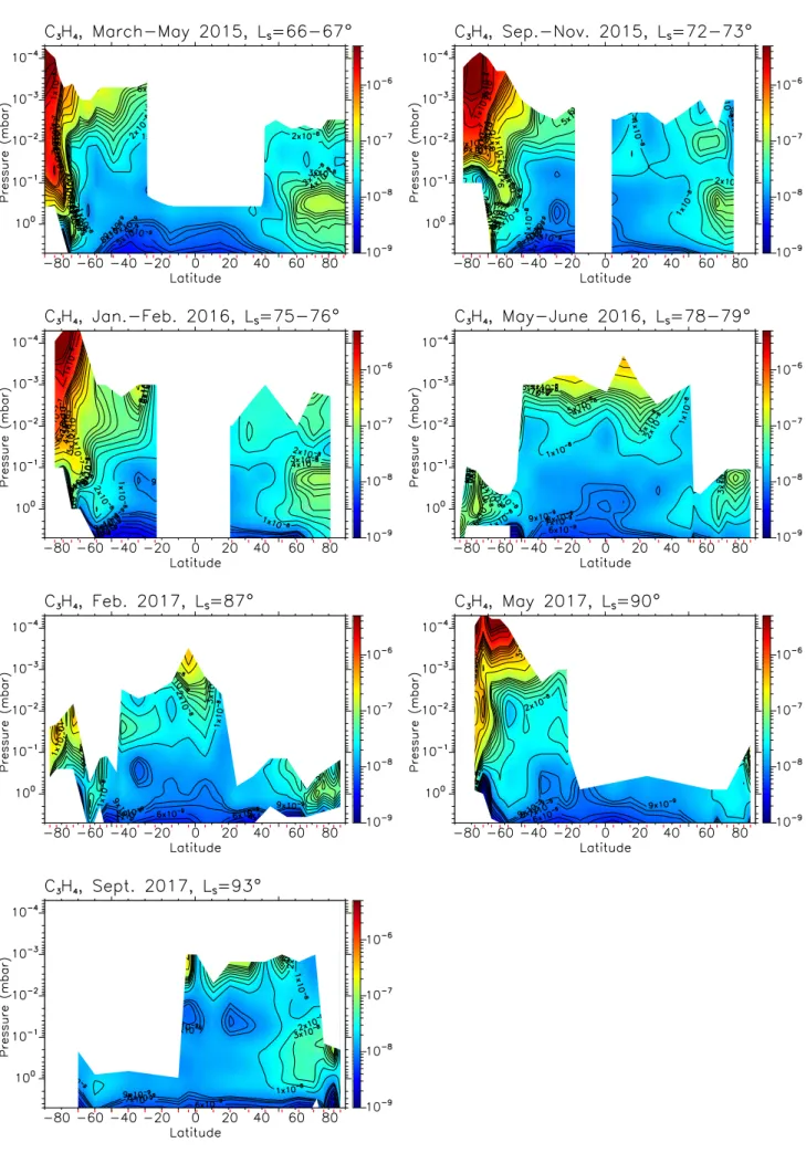
4.2.2. C4H2and CH3C2H VMR meridional cross sections
The molecules C4H2 and CH3C2H (Figs. A.3, A.4, and C.2)
show quite comparable stratospheric and mesospheric VMRs, even though CH3C2H was typically ∼3 times more abundant
than C4H2above the 0.5 mbar level, and the C4H2VMR vertical
gradient is steeper than that of CH3C2H in the deep stratosphere,
between 1 and 5 mbar.
Like other molecules, C4H2 and CH3C2H were strongly
enriched in the southern polar region compared with lower southern latitudes. For instance, in March 2015 at the 0.1 mbar level (∼250 km) the C4H2VMR increased from 10−8at 69◦S to
7 × 10⁻⁷at 84◦S and CH3C2H varyied from 2 × 10⁻⁸to 2 × 10⁻⁶
in the same latitude range. In the mesosphere, at 10−3 mbar,
within the same latitude range, both molecules showed enhance-ment of a factor of 10 in 2015 and in January 2016, and a factor of 5 in May 2017. These enhancements were comparable to those observed for C2H2 and HCN at the same pressure level in the
same period.
At high-northern latitudes, both molecules were locally enriched by a factor of 7 to 9 in a limited zone comprised between 1 and 0.1 mbar and from 50◦N to the pole. In September
2017, after the northern summer solstice, this enriched region seemed to have disappeared for C4H2 and was still observed
for CH3C2H. In contrast to C2H2 and HCN, which showed a
depleted layer at pressures lower than 10−2mbar (as previously
discussed), C4H2 and CH3C2H showed enhancements in this
region.
4.2.3. C2H4, C6H6, HC3N VMR meridional cross sections
C2H4, HC3N, and C6H6 (Figs.A.6,A.7,A.8,C.3, andC.4) are
the molecules that showed the strongest meridional enhance-ments at high-southern latitudes from 2015 to 2017. For instance, in the 10−2–10−3 mbar range these molecules were enriched
between 70◦S and 84◦S by factors of 130, 100, and 40,
respec-tively, with respect to latitudes lower than 65◦S. HC3N and C6H6
were strongly depleted at altitudes lower than 250 km (0.1 mbar) likely due to their condensation. Because of their steep VMR meridional gradient near the south pole, these molecules can be regarded as the best tracers of the polar vortex boundary. In 2015, their VMR cross sections were compatible with a vor-tex boundary that was more confined toward the south pole between 300 and 400 km than at higher and lower altitudes. This gave it an anvil shape for the enriched zone on the maps of Figs. C.3, C.4, with a “tongue” of enriched air extending below 250 km toward lower latitudes. At 1 mbar (Figs.A.6–A.8) this tongue would correspond to a photochemical compound enriched torus enshrouding the polar region and its strato-spheric polar cloud. We note that the tongue is also observed for CH3C2H (Figs.A.4andC.2), C4H2 (A.3andC.2), HCN (A.2
andC.1), and C2H2 (3andC.1). In September 2015, using the
boundary shape of the polar enriched zone we can deduce that the polar vortex was less confined around the south pole and that its boundary seemed to have extended down to almost 60◦S
around 300 km. At this date, and in January 2016, the merid-ional VMR gradients of C2H4, C6H6, and HC3N were less steep
than in March 2015 and their enhancements extended down to 30◦S at high altitude (higher than 300 km). While later (in May
2017) the same high-altitude VMR values were observed beyond 60◦S. This suggests that the polar vortex was at its tightest
latitu-dinal confinement in March 2015, then extended between March and September 2015, and retracted again in early 2016. This evo-lution is similar to the variation of the horizontal extension of the southern polar cloud observed by Cassini/VIMS in the same period (seeLe Mouélic et al. 2018, their Fig.4).
In the northern hemisphere, at latitudes higher than 60◦N and
in the 150–300 km altitude range, these molecules were enriched by factors of 10 to 100 compared to neighboring latitudes and
altitudes. In March 2015 HC3N seemed to present a second
enriched zone above 350 km. The C2H4 VMR showed the most
complex vertical profile at high-northern latitudes with several enriched zones, one in the 250–300 km range and another below 150 km observed in March 2015 and February 2016, while some enrichment was also observed in September 2015 at altitudes higher than 400 km.
4.2.4. Haze mass mixing ratio meridional cross sections We determined the haze mass mixing ratio from the retrieved haze optical depth assuming aerosol composed of 3000 monomers of 0.05 µm radius each (Tomasko et al. 2008) with a bulk density of 0.6 g cm−3. Haze mass mixing ratio cross
sections determined from the 600–620 cm−1continuum thermal
emission (FP3 spectra) are displayed in Figs.4andC.4(middle). They are also compared in Fig.C.4with the haze mass mixing ratio determined from the 1000–1100 cm−1 range acquired by
the FP4. Uncertainties on the continuum at very low radiance levels are responsible for the differences in the meridional cross sections inferred from both focal planes. The haze spatial dis-tribution displays similarities with those of the trace gases; it is strongly enriched in the southern polar vortex (by at least a factor of 10 at 400 km, 10−2mbar) compared to mid-southern latitudes.
At high-northern latitudes the haze is also enriched in a confined region beyond 50◦N and between 1 and 0.1 mbar (200–
300 km), like most of the molecules studied here. Like C2H2,
HCN, and C2H6, the haze mass mixing ratio is depleted in the
northern mesosphere in November 2015, June 2016, and also probably in February 2017, while the mesosphere in May 2015 and September 2017 was enriched in haze. In September 2017, an enriched haze layer was inferred at 10−2mbar (400 km) between
20◦N and 60◦N. This last observation is compatible with the ISS
observation of a haze layer at ∼400 km between 25◦N and 50◦N
at the same date (Seignovert et al. 2020).
The haze mass mixing ratio profile globally increases with height because aerosols are produced in the upper atmosphere and are removed by sedimentation. Interestingly, in March and September 2015, we inferred a depletion in haze in the south-ern polar region below the 0.1 mbar level, where C6H6, HC3N,
and HCN were condensing. This suggests that haze is effi-ciently removed in this region, probably because aerosols serve as condensation seeds for condensing molecules.
4.3. Summary
In summary, in the second part of the southern fall, all pho-tochemical compounds were enriched at the south pole by the subsiding branch of the global circulation cell. By assuming that this enriched air was confined at high-southern latitudes by the polar vortex, the changes in the meridional cross sections of the VMR can be seen as tracers of the horizontal and vertical chang-ing structure of the southern polar vortex. Photochemical species high enhancements combined with the unusually low polar tem-peratures observed in the deep stratosphere resulted in conden-sation between 0.1 and 0.03 mbar (240–280 km) of HCN, HC3N,
C6H6, and possibly C4H2 in March 2015 (Ls=66◦). These
molecules were observed to condense progressively deeper from the south pole. Right outside this condensation zone, the sub-sidence transported the enriched air toward the mid-latitude deep stratosphere probably forming a torus of enriched air enshrouding the polar vortex at 200 km and below.
At high-northern latitudes, stratospheric enrichments rema-ining from the previous winter were observed below 300 km
between 2015 and May 2017 (Ls=90◦) for all chemical
com-pounds, and up to September 2017 (Ls=93◦) for C2H2, C2H4,
CH3C2H, C3H8, and C4H2. These enrichments were observed at
different altitudes depending on the molecule. It was observed at 0.1–0.5 mbar (250–300 km) for the haze, C2H2, C2H4 (with
a more complex vertical structure for C2H4), CH3C2H, C4H2,
and HCN. This pressure region approximately corresponds to the location of the stratopause. In 2015 and 2016, the corresponding C3H8enrichment zone was observed slightly deeper, in the 0.3–
1 mbar pressure range (150–250 km), and even deeper for HC3N,
which was enriched in the 0.5–2 mbar range. C6H6 was also
enriched, but only deeper than the 1 mbar level. In September 2017 these local enhancements were less pronounced than ear-lier for C2H2, C4H2, CH3C2H, HC3N, and HCN, and no longer
observed for C2H6 and C6H6, which suggests a change in the
northern polar dynamics near the summer solstice.
In the mesosphere, C2H2, HCN, and C2H6 were depleted
from the north pole to the mid-southern latitudes, while C4H2,
C3H4, C2H4, and HC3N seem to have been enriched in the
same region. In the deep stratosphere, all molecules except C2H4 were depleted due to their condensation sink located
deeper than 5 mbar outside the southern polar vortex. The HCN, C4H2, and CH3C2H VMR cross section contours showed steep
slopes near mid-latitudes or close to the equator, which can be explained by upwelling air in this region. Upwelling is also supported by the C2H4 enriched air observed in the northern
hemisphere.
5. Discussion
5.1. Thermal field
In the deep stratosphere, our results can be compared with those of Teanby et al.(2019), who inferred the temperature seasonal evolution from CIRS nadir spectra acquired at a spectral reso-lution of 3 cm−1. The temperatures derived in our study at 0.1,
1, and 5 mbar are overall very consistent with their results from 2015 to 2016. A comparison of our thermal field at 5 mbar with results fromSylvestre et al.(2020), who derived temperature at 6 mbar from far-infrared thermal emission acquired by CIRS (using focal plane 1), also shows good consistency.
In our previous study focusing on Titan’s early spring from July 2009 to May 2013 (Vinatier et al. 2015), we were able to infer the pole-to-pole thermal field from December 2009 to February 2012. We recall that from 2012 to 2015 the Cassini orbit inclination prevented us from probing Titan’s polar limbs. The derived thermal field in March 2015 differs greatly from that in 2012 mostly at polar latitudes. The strongest seasonal changes occurred at high-southern latitudes, where a 30 K decrease was derived between 2012 and 2015 in the deep stratosphere together with a 15 K increase at 2 × 10⁻³ mbar. The seasonal
evolution of the thermal field at high-southern latitudes results from a complex interplay between adiabatic heating from the descending branch of the circulation cell and enhanced radia-tive cooling from the enriched molecules, as detailed byTeanby et al.(2017). In 2015, the southern polar vortex was already well established.
The high-northern latitude stratopause was observed about one pressure decade deeper in 2015 than in 2012 and was 5 K warmer. The deeper location of the stratopause at high-northern latitudes could be explained by the combined effect of adiabatic cooling at the 10−2–10−3mbar pressure range by the upwelling
branch of the global circulation, and the increasing mid-spring insolation.
The mid- and low-latitude stratopause was located at the same pressure in 2012 (Vinatier et al. 2015) and 2015, but the 10–20◦N stratopause was 2K colder in 2015 than in 2012 at
0.2–0.3 mbar, which may result from Saturn’s orbit eccentricity (Bézard et al. 2018).
The temperature profiles we derived can be compared with those of Mathé et al.(2020) inferred from CIRS limb spectra acquired at 0.5-cm−1 spectral resolution at comparable
lati-tudes and time. Their dataset probed the same pressure region as ours. The agreement with their mid-northern and high-northern latitude profiles in 2015 and 2016 is very good. Our derived temperatures are also consistent below the mesosphere with their equatorial and mid-southern latitude profiles. How-ever, we derived mesospheric temperatures that were higher by ∼5–10 K than their 2017 equatorial values and their 2016–2017 mid-southern values. At the south pole, our thermal profiles are also in very good agreement with theirs at similar latitudes and longitudes. For instance, in March 2015 Fig.C.1shows that the thermal field is not symmetrical around the south pole with the thermal profile at 81◦S 255◦W (17:58 local time, right-hand side
of the pole in Fig.C.1) showing a stratopause (at 400 km) 12 K warmer than at 78◦S 119◦W (02:52 local time, left-hand side of
the pole in Fig.C.1). As this later thermal profile is in agreement with that inferred byVinatier et al.(2018) and with the results ofMathé et al.(2020) in the 10−2–10−4mbar range, which were
extracted from other CIRS limb data acquired at the same date, longitude, and 15 h apart, it strengthens our derived asymme-try of the thermal field around the south pole in March 2015. This asymmetry probably results from the different insolation conditions between these two limb observations.
5.2. Molecular gas mixing ratio meridional cross sections Our VMR profiles can be compared with the retrieved profiles of Mathé et al.(2020), who used CIRS limb spectra acquired at 0.5 cm−1 over the entire Cassini mission. Our retrieved
VMR profiles are overall in very good agreement with their results. For instance, at high-northern latitude, they also inferred similar local VMR maxima for C2H2 and HCN in the 0.1–
1 mbar pressure range, they derived a local VMR minimum at ∼0.005 mbar with equivalent VMR values. Other VMR profiles that we derived in this study are also consistent with their results, except at 81◦S–125◦W in March 2015 as they retrieved C2H2and
HCN VMR 10 times higher than ours at and above 10−4mbar,
while our profiles agree deeper than this pressure level for C2H2.
However, at this location, other molecular VMRs are consistent within the error bars. These observations have larger uncertain-ties than any other because of the low temperature there, which can explain discrepancies between the two studies.
The mixing ratios we retrieved around 1 mbar can be com-pared with those retrieved byTeanby et al.(2019) andCoustenis et al. (2020), who inferred VMRs from CIRS nadir spectra acquired at 2.5 and 0.5 cm−1 spectral resolution, respectively.
Common molecules between our study andTeanby et al.(2019) are C2H2, C2H4, C2H6, CH3C2H, C4H2, HCN, and HC3N;
Coustenis et al.(2020) additionally retrieved VMR of C3H8and
C6H6. As vertical information is very limited from nadir
obser-vations, both studies assumed constant-with-height mixing ratio profiles above the condensation level, which makes a detailed comparison partially meaningful as our derived profiles show strong vertical variations with altitude. Nevertheless, around 1 mbar the relative decrease in molecular VMRs at the north pole and their relative increase at the south pole (Teanby et al. 2019) in the 2015–2017 period in is overall agreement with our
results. However, because of their constant-with-height VMR assumption, these authors could not derive the local enhance-ment that we inferred at high-northern latitude in the 1–0.1 mbar pressure range. In general, our stratospheric (in the 5–0.5 mbar range) inferred VMR are in good agreement with those derived byCoustenis et al.(2020).
We derived the highest VMR in the south pole mesosphere in March 2015, when the polar vortex was at its tightest latitudi-nal confinement. Our derived VMRs of C2H2, HCN, CH3C2H,
and C4H2 inside the polar vortex at 600 km (2 × 10⁻⁵mbar) are
similar to the VMRs measured in situ by the Cassini Ion Neu-tral Mass Spectrometer (INMS) above 1000 km (Vuitton et al. 2007;Cui et al. 2009;Magee et al. 2009). This observation, also reported byMathé et al.(2020), suggests that subsidence at the south pole transports enriched air from altitudes much higher than 600 km. Additionally, the derived thermal zonal wind (see Sect.5.5) also supports a more confined polar vortex in March 2015 with winds of ∼240 m s−1reaching at least 600 km, with
subsidence therefore necessarily coming from higher altitudes. The only molecule among all those studied here that does not condense in Titan’s atmosphere is C2H4. This explains why
it is enriched in the deep stratosphere by advection from the fall–winter polar region towards the spring–summer pole in the deep atmosphere by the deep branch of the global circulation (Vatant d’Ollone 2020). Additionally, C2H4is photodissociated
below 500 km and reacts with H atoms to form C2H5 (Vuitton
et al. 2019), which can explain its depletion at mid- and low lati-tudes above 150 km. The global northern hemisphere enrichment compared to the southern hemisphere below 300 km observed since November 2015 (Ls= 73◦) could be explained by a global
vertical transport of this molecule at mid- and high-northern lat-itudes, which is compatible with the spring and summer ascend-ing branch predicted by GCMs (e.g.,Vatant d’Ollone 2020). The complex northern polar structure of its VMR meridional cross section suggests a complex circulation pattern, perhaps includ-ing two small circulation cells that could have coexisted in 2015 and 2016, keeping the C2H4 enrichments in two distinct
alti-tude ranges (one around 0.1 mbar and another one deeper than 1 mbar).
5.3. Local mesospheric minimum VMR of C2H2, C2H6, and
HCN
According to Vuitton et al. (2019), the predicted lifetimes of C2H2, C2H6, and HCN in the mesosphere are mostly controlled
by vertical transport timescales, resulting in lifetimes of 14 Titan days (230 days) at 500 km (∼10−3 mbar) for C2H2, 100 Titan
days for C2H6, and 1000 Titan days for HCN. Chemical
life-times decrease with altitude, and it is possible that the observed mesospheric depleted air comes from higher levels where these molecules are more efficiently photodissociated. Assuming that the C2H2- and HCN-depleted air observed at 80◦N on May 9,
2015, was horizontally advected to 40◦S on September 29, 2015,
would imply an horizontal advection of 50 cm s−1, a value higher
but not so far from the 0.1–0.2 m s−1predicted by the IPSL Titan
GCM in diurnal average (Vatant d’Ollone 2020;Vatant d’Ollone et al. 2018). Using the continuity equation, this horizontal veloc-ity would imply a subsidence vertical velocveloc-ity of ∼3 mm s−1
inside the southern polar vortex at 10−2mbar (∼400 km), which
is consistent with estimations ofTeanby et al. (2017) in 2015 using a radiative model and from their derived mixing ratio pro-files. Another possibility to explain the presence of this depleted zone could be diurnal effects, which is at odds with the conclu-sion ofVuitton et al.(2019). We observe a correlation between
the mesospheric temperature maximum observed during the day (displayed in yellow and orange in Figs.2andC.1) and the lower VMRs of C2H2, C2H6, and HCN. Instead, during the nighttime
the mesospheric VMRs seemed to be enhanced. This hypothesis needs other data analysis to be confirmed or refuted.
5.4. Haze extinction meridional cross sections: comparison with ISS observations
Seignovert et al.(2020) derived the seasonal variation of Titan’s haze extinction from October 2004 to September 2017 in the 350–550 km altitude range from the analysis of the Cassini Image Sub-System Narrow Angle Camera in the CL1-UV3 UV filter at 338 nm. We can compare the spatial distribu-tion of extincdistribu-tion we derived from CIRS in the 350–450 km range, which is generally the overlap altitude range probed by UV and thermal infrared observations.Seignovert et al.(2020) inferred complex temporal variation of the haze extinction in the stratopause and mesospheric levels with high temporal vari-ability. In order to compare haze extinction coefficients derived from CIRS observations at 1090 cm−1 and the UVIS ones at
338 nm (29 586 cm−1), we applied a multiplicative factor equal
to 1.22 × 10⁻³ derived from the far-IR to UV spectral
depen-dence of the aerosol cross sections ofVinatier et al.(2012, see Fig. 2 therein). A comparison of our haze extinction coefficient maps with those derived from ISS observations acquired at sim-ilar dates is displayed in AppendixD. In the overlapping altitude range, agreement is overall within a factor of 2, which is typi-cally the uncertainty on the haze extinction coefficient derived from CIRS limb spectra above 350 km. The largest difference is inferred in September 2017, which corresponds to an ISS obser-vation with a limited latitudinal coverage for which Titan’s center adjustment, and therefore the altitude grid extraction, is not as well constrained as for other ISS datasets (seeSeignovert et al. 2020).
5.5. Thermal winds
Performing a scale analysis for Titan’s parameters of the differ-ent terms of the momdiffer-entum equation in spherical coordinates projected over the northward direction gives the remaining terms: 2Ωsin(φ)u + tan(φ) r u2+ 1 ρr ∂p ∂φ z =0.
Here u is the zonal wind velocity (eastward), Ω the rotation rate of Titan, r the sum of Titan’s radius and altitude, φ the latitude, p the pressure, and ρ the atmospheric number density. Frictional forces can be neglected in the stratosphere. Appendix E gives solutions of this equation that we applied to calculate u from the meridional pressure gradient. Titan’s zonal winds were previ-ously determined from the thermal field derived from CIRS limb and nadir observations by Flasar et al. (2005) andAchterberg et al. (2008) during Titan’s northern winter, by Achterberg et al. (2011) from winter to northern spring, and extended by Achterberg et al.(2018) over early northern summer but deeper than 0.05 mbar as they used CIRS nadir datasets. Our zonal wind integration differs from these previous studies as we did not integrate the thermal wind equation over cylinders concen-tric around Titan’s rotation axis (Flasar et al. 2005), but instead performed integration in spherical coordinates (see AppendixE). We set the zonal wind at 5 mbar to 120 m s−1, which is
com-patible with in situ measurements acquired by the Doppler Wind
Experiment aboard Huygens during the probe descent (Bird et al. 2005;Folkner et al. 2006).
Figure5shows the meridional cross sections of zonal wind velocity (eastward) derived from the thermal fields displayed in Fig.2. During the studied period all the derived meridional cross sections of zonal wind show a clear asymmetry between the northern and southern hemispheres with zonal winds much faster in the southern hemisphere than in the northern one. If we consider that the southern polar vortex boundary is characterized by the strongest zonal winds around the south pole (circumpo-lar jet reaching 240–280 m s−1), our derived zonal wind maps
in March 2015 and September 2015 show that the polar vortex was confined to latitudes higher than 70◦S in March and 60◦S in
September. This horizontal extension is consistent with results from the VMR cross sections that display the same latitudinal extension of the enriched zone between the two dates (see, e.g., Fig.A.2). In 2016 the high-southern latitude jet seemed to slow down while migrating toward low-southern latitudes in June 2016 and February 2017. A less pronounced zonal wind local maximum was derived at 65◦S at ∼10−2mbar in June 2016 and
February and May 2017. Such temporal evolution of zonal winds can explain the temporal change in the VMR enrichment patterns at high-southern latitude described in Sect.4.2, confirming that they are linked to the polar vortex changing structure.
In all of our derived stratospheric wind maps, the north-ern zonal winds are much weaker than the southnorth-ern hemisphere winds with values typically lower than 160 m s−1, which is (given
the studied period) totally consistent with momentum conserva-tion in a superrotating atmosphere overturning cell leading to faster winds during autumn and winter in altitude. The north-ern wind speeds seemed to be globally higher in the deep stratosphere (deeper than 10−1mbar) than above the stratopause
(above 10−1mbar). This last point, added to the fact mentioned
previously that the stratopause seems to be an area of limited mixing for some species, supports the idea (supported by mod-els such as the ISPL Titan GCM) that the stratopause could act as a separation between stratospheric and mesospheric cir-culation pattern (Vatant d’Ollone 2020; Vatant d’Ollone et al. 2018).
We can compare our derived zonal wind cross section with the one derived by Achterberg et al.(2018) in 2016 and 2017. Their maps are determined below the 0.05 mbar level because they were calculated from thermal fields inferred from CIRS nadir observations. Below this pressure range, our derived zonal wind horizontal and vertical structures are in good agreement.
Lellouch et al. (2019) determined zonal wind velocities in July and August 2016 from the Doppler shifts of submillime-ter lines for several molecules acquired by ALMA (Atacama Large Submillimeter Array) interferometer. From all their stud-ied molecules, which probe different levels in the atmosphere, they derived wind maps with faster zonal winds in the south-ern hemisphere than in the northsouth-ern hemisphere, along with an equatorial jet. Our derived thermal wind structures in May 2016 are overall in very good agreement with their measure-ments as we derive wind values at 20◦S (240–260 m s−1 in
the 300–600 km range, or in the 0.1–10−4mbar pressure range)
comparable to their fitted values assuming solid-body rotation (210 m s−1 between 200 and 400 km, and 260–290 m s−1
between 400 and 700 km). Our larger zonal wind observed at low-southern latitudes in May 2016 (and probably also in Febru-ary and May 2017) is consistent with theLellouch et al.(2019) direct detection of an equatorial jet in August 2016. It should be noted, however, that for latitudes lower than 20◦ the q 1
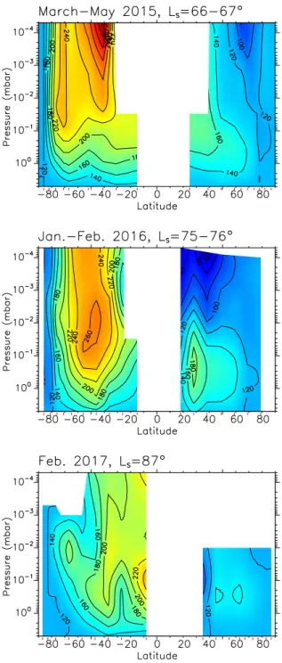
Fig. 5.Zonal wind cross sections from March 2015 to September 2017. Contours are given every 20 m s−1; the color scale is the same for all
plots. Regions without information are represented in white. They correspond to missing data, pressure levels not probed by nadir observations, or regions not used to perform the wind calculation at low latitudes.
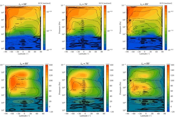
−90 −60 −30 0 30 60 90 Latitude (∘) 10 1 100 101 102 103 104 105 P re ss ure (P a) -0.0030 -0.0010 -0.0100 -0.0100 -0.0300 -0.0100 -0.0300 -0.010 0 -0.0300 -0.0300 -0.1000 -0.1000 -0.0300 0.0100 Ls= 68∘ 10−8.0 10−7.0 10−6.0 HCN [mol/mol] −90 −60 −30 0 30 60 90 Latitude (∘) 10 1 100 101 102 103 104 105 P re ss ure (P a) -0.0010 -0.0030 -0.0010 -0.0030 -0.0010 -0.00 30 -0.0100 -0.0300 -0.1000 -0.0300 -0.010 0 -0.0100 -0.0300 -0.0300 -0.0300 -0.0300 Ls= 76∘ 10−8.0 10−7.0 10−6.0 HCN [mol/mol] −90 −60 −30 0 30 60 90 Latitude (∘) 10 1 100 101 102 103 104 105 P re ss ure (P a) -0.0010 -0.00 10 -0.003 0 -0.0100 -0.0300 -0.0300 -0.0300 -0.0300 -0.1000 -0.03 00 -0.0300 -0.0100 -0.0030 -0.001 0 -0.0300 -0.0300 -0.1000 -0.1000-0.1000 -0.1000 Ls= 89∘ 10−8.0 10−7.0 10−6.0 HCN [mol/mol] −90 −60 −30 0 30 60 90 Latitude (∘) 10−1 100 101 102 103 104 105 Pre ssure (P a) -0.0100 -0.00 30 -0.0010 -0.0100 -0.010 0 -0.0300 -0.0300 -0.0100 Ls= 68∘ −20 0 20 40 60 80 100 120 140 160 u [m/s] −90 −60 −30 0 30 60 90 Latitude (∘) 10−1 100 101 102 103 104 105 Pre ssure (P a) -0.001 0 -0.0 030 -0.0010 -0.0030 -0.0010 -0.0030 -0.01 00 -0.0100 -0.0100 -0.0300 -0.0300 -0.0300 -0.1000 Ls= 76∘ −20 0 20 40 60 80 100 120 140 160 u [m/s] −90 −60 −30 0 30 60 90 Latitude (∘) 10−1 100 101 102 103 104 105 Pre ssure (P a) -0.0010 -0.0 010 -0.00 30 -0.0100 -0.0300 -0.0300 -0.0100 -0.0300 -0.0030 -0.0010 -0.0300 -0.0300 -0.1000 -0.0300 Ls= 89∘ −20 0 20 40 60 80 100 120 140 160 u [m/s]
Fig. 6. Predictions of the IPSL Titan GCM for HCN volume mixing ratio (top) and the zonal wind (m s−1, bottom) for Ls= 68, 76, and
89◦. Meridional circulation is superimposed with stream functions (109 kg s−1) in solid lines for clockwise circulation and dotted lines for
counterclockwise.
term in the zonal wind solution (see Appendix E) can amplify uncertainties on our derived wind profiles.
Our results show that two years before the southern winter solstice, the southern polar vortex structure was changing within a few Titan days, resulting in more or less pronounced molec-ular enhancements inside the polar vortex. One year before the summer solstice, two jets are derived in the southern stratosphere near 70◦S and at mid-southern latitudes.
5.6. Comparison with the Institut Pierre Simon Laplace Titan Global Climate Model
Our VMR meridional cross sections can be compared with the predictions of the IPSL Titan GCM. This GCM, which has been recently upgraded to take into account coupling between chem-istry, radiative transfer, haze microphysics, and global dynamics (Vatant d’Ollone 2020;Vatant d’Ollone et al. 2018), is currently the most complete. It models processes occurring in the middle atmosphere of Titan.
Figure6 shows the predicted HCN VMR (top) and zonal wind (bottom) for Ls=68◦, 76◦, and 89◦, with corresponding
stream functions for each season. At mid- and low latitudes, the molecular depletion that we observe in the deep stratosphere is predicted by the GCM to result from air ascending from condensation levels (see the predicted VMR in the 102–103 Pa
region).
The northern winter residual circulation cell is predicted to extend from the north pole to ∼50◦N in the deep stratosphere
and decrease in size with time, before vanishing around the
northern summer solstice. Seasonal change of this residual cir-culation cell was responsible for the maintenance of the local northern polar stratospheric enhancements during spring. This result from the GCM, although predicted at deeper levels than observed here, could explain our local gas VMR and haze mass mixing ratio enrichment at the north pole deeper than 0.1 mbar, which slowly dissipated after the northern summer solstice. The IPSL Titan GCM also predicts that the southern mesosphere is more enriched in photochemical products than the northern mesosphere. This tendency is also observed here; however, we inferred southern enhancements that are more confined around the south pole than the GCM prediction before the southern sum-mer solstice. This difference can be explained by the GCM top layer located at 10−1Pa, which limits the vertical extension of the
meridional circulation along with the horizontal resolution used in the model, which is too low to reproduce steep meridional gra-dients. Despite these limitations, the IPSL Titan GCM predicts a high-southern latitude mesosphere (above the 10 Pa level) that is more enriched than earlier in photochemical compounds near the summer solstice, combined with a light depletion of polar air deeper than 10 Pa. This prediction is also in agreement with our observations, even though observed in a lower pressure range.
As in most of the models, predicted zonal winds for northern spring and summer are faster in the southern hemisphere than is the northern. Structure of the southern polar vortex is predicted to change within the observing time studied here, with a global decrease in zonal wind speed with time and development of a double equatorial jet, a stratospheric and a mesospheric. This predicted complex seasonal variation of the zonal wind is in very