Detection statistics for multichannel data

Detection Statistics for Multichannel Data

RLE Technical Report No. 550

December 1989

Tae Hong Joo

Research Laboratory of Electronics

Massachusetts Institute of Technology

Cambridge, MA 02139 USA

This work was supported in part by the Defense Advanced Research Projects Agency

monitored by the Office of Naval Research under Grant No. N00014-89-J-1489,

in part by the National Science Foundation under Grant No. MIP 87-14969, in part

by Sanders Associates, Incorporated, and in part by a fellowship from the Amoco

©

Massachusetts Institute of Technology. 1989. All rights reserved.

Detection Statistics for Multichannel Data

by

Tae Hong Joo

Submitted to the Department of Electrical Engineering and Computer Science on September 9, 1989, in partial fulfillment of the

requirements for the degree of Doctor of Philosophy

Abstract

A new detection statistic is developed for a class of multichannel detection problems which have the requirement that in the presence of an emitter, a narrowband signal must exist in all channels in addition to wideband noise. When an emitter is absent, the received data may contain narrowband noise components in some, but not all of the channels, as well as wideband noise. A detector which tests each channel separately for the existence of the narrowband component does not perform as well as the detectors which use all channels collectively.

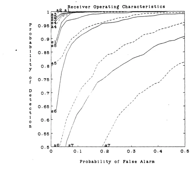
To collectively use the data from different channels, average has been previously used as a detection statistic. However, because the average tests only the total energy, its detection performance noticeably degrades when a narrowband component exists in many channels. As an alternative detection statistic, the semblance, which measures the coherence between the channels, is considered. The receiver operating characteristic curves show that the average performs better than the semblance if more than half of the channels contain only wideband noise when the emitter is absent, while the semblance performs better than the average if more than half of the channels contain narrowband components when the emitter is absent. Therefore, the detection performance of both the average and the semblance can be improved. An improved detection statistic is developed by combining the average and the semblance. A combining function is determined by satisfying a set of constraints which ensure that the average and the semblance contribute equally to the detection statistic. Before they are combined, the average is transformed to make its probability density function match the probability density function of the semblance. The receiver operating characteristic curves show that the combined statistic performs better than other statistics including the average and the semblance.

This new detection statistic is applied to the gravitational wave signal detection problem. A new algorithm which computes the Fourier transform magnitudes at the exact frequencies using the chirp z-transform is developed. Examples of the gravitational wave signal detection are presented to demonstrate that the new algorithm performs better than the existing algorithm. Thesis Supervisor: Alan V. Oppenheim

Title: Professor, Department of Electrical Engineering and Computer Science

__ ·

~

_l- 1_

To Leslie

-Acknowledgements

This thesis represents the conclusion of my long and circuitous career as a graduate student. This would not have been possible without the support of my friends and family. I would like to acknowledge their help.

I express my sincere gratitude to my advisor, Prof. Al Oppenheim, who arranged the finan-cial support with unrestricted freedom and guided me through the challenges of the research. I am grateful to Al for his confidence in me and I thank him for all the metaphors. The best part of the doctoral program has been the privilege of working with him.

Prof. Rainer Weiss and Prof. Bruce Musicus served as thesis readers. Bruce suggested the multiple hypothesis testing idea and made many helpful comments. Prof. Weiss provided the gravitational wave data, hence the initial motivation for the multichannel detection prob-lem. Dr. Jeffery Livas introduced me to the gravitational wave signal processing problem and generously answered many questions in the early stage of this research.

Deborah Gage made the Digital Signal Processing Group a nice place to work. Giovanni Aliberti maintained the computers in excellent shape and taught me about them.

Doug Mook encouraged me with his enthusiasm and interest in my work in addition to finding summer jobs for me at Sanders. Peter Doerschuk was always available to discuss many ideas and provide helpful suggestions. Rick Lamb frequently restored my balance by providing bizarre perspectives on life.

Michele Covell and Daniel Cobra, fellow graduate students who are also completing their theses, provided encouragement through their diligence to finish. I also thank the past and the present members of the Digital Signal Processing Group for making it a stimulating place to do research.

During the course of my study, I received generous financial support from the Advanced Research Projects Agency monitored by the Office of Naval Research, the National Science Foundation, Sanders Associates, Inc., and the Amoco Foundation.

My mother, Ja-Ok Kim Joo, and my brother, Tae-Young Joo, have provided unlimited, steadfast support throughout my study. I am grateful to them.

Finally, my wife, Leslie Reade Schenck, deserves my deepest appreciation. Leslie has sup-ported and encouraged me with her unbounded love. Without her, it would not have been as fun or as meaningful. I dedicate this thesis to Leslie with love.

4

Contents

Abstract Acknowledgments 4 List of Figures 7 List of Tables 8 1 Introduction 9 1.1 Problem Statement ... ... ... 9

1.2 Overview of the Thesis ... 10

2 Multichannel Detection Problem 14 2.1 Problem Statement ... 14

2.2 Detection Based on a Series of Binary Hypothesis Tests . ... 15

2.3 Binary Hypothesis Testing ... 18

2.3.1 Detection Statistic ... ... 19

2.3.2 Receiver Operating Characteristic ... 20

2.4 FFT Coefficient Quantization Effects on Detection . ... 23

2.4.1 Coefficient Quantization ... 23

2.4.2 Probability of Detection using Quantized Coefficients ... . 29

2.5 Deficiency of Detection Based on a Series of Binary Hypothesis Tests ... . 30

2.6 Summary ... ... ... 32

3 Multichannel Detection Statistics 33 3.1 Average . . . .. . . 33

3.1.1 Multichannel Binary Hypothesis Testing Problem ... 34

3.1.2 Approximation of Probability Density Functions . . . ... 36

3.2 Semblance .... ... . ... ... 38

3.2.1 Background . ... 39

3.2.2 Properties ... .... ... 39

3.2.3 Derivation of Probability Density Functions ... 40

3.2.4 Approximation of Probability Density Functions using the Beta Proba-bility Density ... ... 43

3.3 Numerical Evaluation of Detection Statistics . ... 47

5

3.4 3.5 3.6 3.A

3.3.1 Monte Carlo Integration for Receiver Operating Characteristic ... 48

3.3.2 Monte Carlo Detection Computation ... .. 50

Examples of Receiver Operating Characteristic . ... 51

Alternate Multiple Hypothesis Testing Formulation . ... 54

Summary ... 57

Semblance Properties ... 59

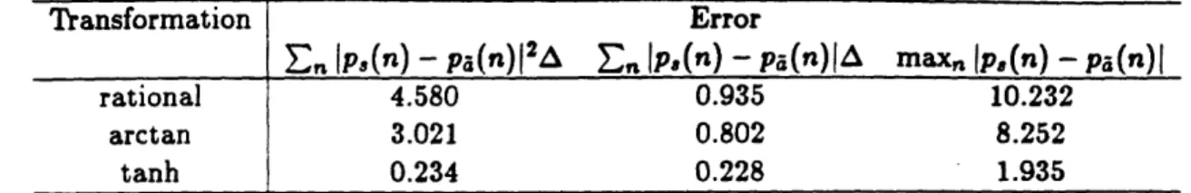
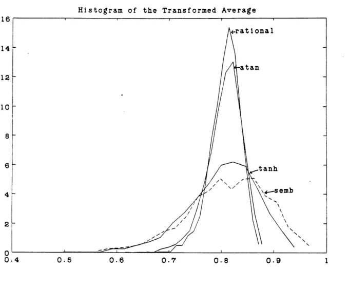
4 Combining Average and Semblance 61 4.1 Combining Average and Semblance Using Probability Density Function Matching 62 4.1.1 Probability Density Function Matching by Transform Functions ... 64

4.1.2 Probability Density Function Matching based on Cumulative Distribution Function ... 66

4.2 Combining Average and Semblance Using Likelihood Ratio . ... 68

4.3 Combining Average and Semblance Using Discriminant Functions . ... 72

4.3.1 Gaussian Classifier ... 72

4.3.2 Quadratic Classifier ... 72

4.4 Performance Comparison ... 73

4.5 Summary ... 78

4.A Combining Average and Semblance using the Likelihood Ratio Test: General Case 80 5 Gravitational Wave Signal Detection 5.1 Background. 5.2 Description of Received Gravitational Wave Signal. 5.3 Detection Using the Measured Data ... 5.4 Previous Detection Algorithm ... 5.5 New Algorithm for Estimating the Narrowband Component 5.6 Comparison ... 5.7 Summary ... 6 Summary and Future Research 6.1 Summary ... 6.2 Suggestions for Future Research . 83 . ... .84 . ... .86 . ... .89 . ... .92 . ... .93 . ... .96 ... .101 103 ... ... 103 ... 105 Bibliography 109 6 _ _I

List of Figures

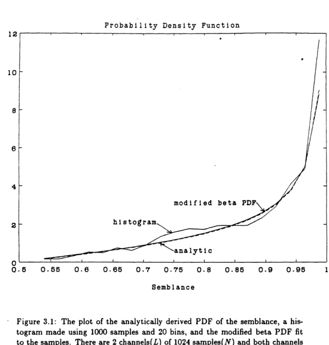
2.1 The maximum magnitude error of the FFT using quantized coefficients ... 28 2.2 The probability of detection of the FFT using quantized coefficients ... 31 3.1 The probability density function of the semblance, a histogram and the modified

beta function approximation: simple case ... ... 42 3.2 A histogram and the modified beta function approximation of the semblance:

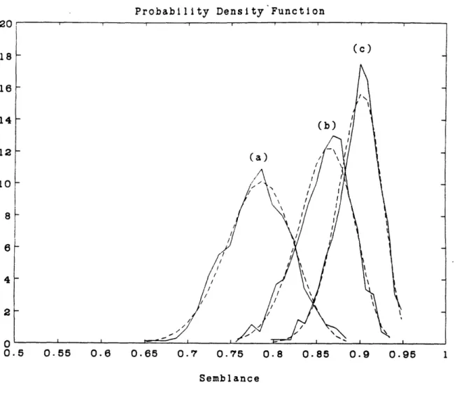
general case ... ... 46 3.3 Receiver operating characteristic curves of the average and the semblance .... 53 4.1 Histograms of the transformed averages using different transform functions and

a histogram of the semblance ... 67 4.2 A histogram of the transformed average using the CDF matching method and a

histogram of the semblance ... 69 4.3 Comparison of receiver operating characteristics: 2 channel case ... 75 4.4 Comparison of receiver operating characteristics: the narrowband component in

2 of 8 channels under the Ho hypothesis case . ... 76 4.5 Comparison of receiver operating characteristics: the narrowband component in

4 of 8 channels under the Ho hypothesis case ... . 77 4.6 Comparison of receiver operating characteristics: the narrowband component in

6 of 8 channels under the Ho hypothesis case . ... 79 5.1 The coordinate system used for gravitational wave detection ... 87 5.2 The instantaneous frequency of the received gravitational wave signal ... 90 5.3 Computation of the Fourier transform magnitudes using the chirp z-transform. . 95 5.4 The detection statistic of the Livas algorithm . . . 99 5.5 The detection statistic of the new algorithm .. ... .. ...100 5.6 Receiver operating characteristic curves of the Livas algorithm and the new

al-gorithm ... 102

7

List of Tables

2.1 The maximum magnitude error of the FFT using quantized coefficients ... 27

3.1 X2 fit test of the modified beta function approximation ... . 48

3.2 The probability of false alarm of the Monte Carlo detector ... 52

4.1 Errors of the probability density function mapping ... 66

5.1 Constants used in the gravitational wave signal detection ... 89

5.2 The starting times of the gravitational wave data set. ... 91

5.3 Comparison of the Fourier transform magnitude computation ... . 98

8

Chapter 1

Introduction

1.1

Problem Statement

Multichannel signal detection using a receiver array arises in a variety of contexts such as the gravitational wave signal detection problem. Although a gravitational wave is a steady-state signal, it is measured in short bursts because of constraints imposed by the receiver hardware and local noise. The measurement is interpreted as multichannel data by treating each burst of measurement as the output of a channel of a multichannel receiver. When a gravitational wave is measured on earth, the received signal is frequency modulated due to the relative motion between the emitter and the receiver and is contaminated by local disturbances, some of which are narrowband noises. Local narrowband noises exist intermittently or have a constant frequency. If a gravitational wave emitter is present, the gravitational wave signal should exist in all channels of the receiver and the frequency of the signal should be modulated according to the emitter location and frequency. Therefore, the detector must use the existence of the signal with varying frequency in each channel to distinguish the gravitational wave signal from the false alarms caused by local narrowband noise sources.

The frequency variation of the signal over the channels is dependent on the particular detection problem. However, the requirement that the signal exists in all channels in order to decide that an emitter is present is common in many multichannel narrowband signal detection problems. Therefore, the detection problem is formulated as the following hypothesis testing

9

X·---·---problem:

S1 + WL

H

1

(emitter is present): R=

SL + WL

Ho (emitter is absent):

R

i

sL + WL

where R denotes the received data, A is the sinusoidal signal vector A cos(wln + 0b) for n =

0, 1, .. , N-

in the Ith channel, and w is the noise vector in the Ith channel for I = 1, 2, * , L.

The amplitude of the sinusoidal signal, A, is the same for all channels and the frequency

and the phase vary over the channels. For the Ho hypothesis, the received data can also

contain the narrowband component in some channels because of intermittent narrowband noise.

Unfortunately, the exact number and identity of the channels which contain the narrowband

component are unknown, therefore, the conventional likelihood ratio detector cannot be used.

This composite binary hypothesis testing problem can be formulated as a series of single

channel binary hypothesis tests. However, because all channels are not considered collectively,

the existence of a consistent signal in the channels is not explicitly checked. Thus, one purpose

of this thesis is to develop improved algorithms for this detection problem and apply them to

the gravitational wave signal detection problem.

1.2

Overview of the Thesis

If the received data under the Ho hypothesis contain only wideband noise, the likelihood

ratio detection statistic for the hypothesis testing problem is the average of the maximum value

of the Fourier transform magnitude in each channel. However, when the received data contain

narrowband noise, the average performs poorly even though it uses all channels collectively.

Therefore, the semblance will be considered as the detection statistic to correct this shortcoming.

Semblance is the ratio of the power of the sum of the spectra and the sum of the powers

of the individual spectra and is related to the normalized cross-correlation. It is sensitive

to the existence of the signal and is, therefore, well matched to the requirement that the

signal must exist in all channels for the H

1

hypothesis. Because the semblance measures the

10

coherence of the signals, it employs fundamentally different criterion than the detectors which

employ averaging. Unfortunately, noise alone can produce a high semblance value because the

semblance is insensitive to the power of the signal. To take advantage of the sensitivity of the

semblance to the correlation between channels and of the sensitivity of the average to the signal

power, new detection statistics will be developed by combining the semblance and the average.

The combined statistic will be applied to the measured gravitational wave data to demonstrate

its effectiveness.

The gravity wave signal detection problem is representative of a large class of multichannel

detection problems which have a strict requirement that all channels must contain the signal

in order to correctly decide that an emitter is present. While this thesis focuses on the

gravita-tional wave signal detection problem, the results on detection statistics are applicable to other

multichannel signal detection problems.

The goal of the gravitational wave signal processing is to accurately and efficiently detect

frequency-modulated, periodic gravitational wave signals with unknown emitter location and

frequency. Because the emitter parameters are unknown, the gravitational wave detection

al-gorithms first hypothesize a location and frequency, then detect the hypothesized emitter. The

algorithm must test for all directions and all frequencies and is, therefore, computationally

intensive. Fortunately, however, an algorithm can be developed which tests all possible

fre-quencies simultaneously once the emitter location is selected. Because selecting the emitter

location and frequency uniquely specifies the instantaneous frequency of the received signal,

the periodic gravitational wave detection algorithm is implemented in two parts. First, the

signal component of the hypothesized emitter in each channel is computed where the signal

component is taken to be the Fourier transform magnitude at the frequencies predicted by the

emitter location. Second, the magnitudes are used to compute the detection statistic which is

a combination of the average and the semblance.

Contributions of the Thesis

First, the multichannel detection problem is formulated as a series of single channel binary

hypothesis tests. The generalized likelihood ratio detector for each binary hypothesis test is

efficiently implemented by the FFT. Because only the arithmetic computational error of the

11

1_ __ I

-X-ll-ll---FFT has been analyzed previously, a deterministic analysis of the -X-ll-ll---FFT coefficient quantization effect on the FFT detector is developed.

Second, the average and the semblance are separately used as a multichannel detection statistic because they use data from all channels collectively. The semblance has been previously used as a detection statistic but its probability density function was unknown. A closed form expression of the probability density function of the semblance is developed for a simple case and a very accurate approximation is developed for the general case.

Third, a new detection statistic with improved detection performance is formed by combin-ing the average and the semblance. A general method of combincombin-ing two statistics which have different detection characteristics is developed. This method combines the statistics by satisfy-ing a set of functional constraints. Improved detection probability of the combined statistic is demonstrated by comparing it with the average and the semblance.

Fourth, the new statistic, formed by combing the average and the semblance, is applied to the gravitational wave signal detection problem. Before the detection statistic can be applied, the Fourier transform magnitudes must be computed. A more accurate algorithm which uses the chirp z-transform to compute the Fourier transform magnitudes at the exact frequency locations is developed. This new algorithm and the combined statistic are used to process the measured gravitational wave data.

Outline of the Thesis

Chapter 2 begins with a formal statement of the multichannel signal detection problem. By enumerating all possible hypotheses, a detector based on a series of single channel binary hypothesis tests is developed. A solution to the binary hypothesis testing problem is reviewed. It is shown that the FFT provides an efficient implementation of the solution. The effect of quantized FFT coefficients on detection is examined using a deterministic error analysis of the quantized FFT coefficients. Chapter 2 ends with a discussion of the deficiencies of the detection based on a series of binary hypothesis tests.

Chapter 3 includes a discussion of the average and the semblance as detection statistics. The average is the likelihood ratio test solution to the multichannel hypothesis testing problem with the received data containing only wideband noise for the Ho hypothesis. The receiver operating

12

characteristic computation is reviewed. Next, the semblance is introduced and its properties are reviewed. The probability density function of the semblance is analytically derived for a simple case and is approximated using the modified beta probability density function for the general case. To evaluate the effectiveness of the average and the semblance as detection statistics, their receiver operating characteristics are estimated using the Monte Carlo detection computation. A comparison of the average and the semblance as the detection statistics of the multichannel hypothesis testing problem is provided. Chapter 3 ends with a new multiple hypothesis testing formulation of the detection problem which suggests a detection statistic that is a combination of the average and the semblance.

Chapter 4 develops different methods of combining the average and the semblance because the detection performance of individual statistics can be improved. The statistics are combined by satisfying a set of intuitive functional constraints. The likelihood ratio combination can be derived for a simple case and is used to evaluate the previous method of combining statistics. For the general case, a combination using the discriminant function method is developed. Chapter 4 ends with a comparison of the detection statistics.

Chapter 5 provides a detailed discussion of gravitational wave signal processing. A descrip-tion of the received signal and the existing detecdescrip-tion algorithm are reviewed. A new algorithm which does not have the shortcomings of the existing algorithm is developed and is applied to the gravitational wave data. Chapter 5 ends with a comparison of the previous algorithm to the new algorithm to show that the new algorithm performs better.

Chapter 6 concludes the thesis by presenting a summary and suggestions for future research.

13

__·_ __ 11

-_---Chapter 2

Multichannel Detection Problem

In this chapter, a particular type of multichannel detection problem is discussed. Because a simple model of the received data when an emitter is absent is not available for the detection problem, a detector based on a series of single channel binary hypothesis tests is proposed. A single channel binary hypothesis test is efficiently implemented using the FFT. Because of the crucial role played by the FFT, the effect of inaccuracies in the FFT coefficients on the detector performance is analyzed. Lastly, the receiver operating characteristic of the detector based on a series of binary hypothesis tests is determined and the deficiencies of the detector are discussed.

2.1

Problem Statement

Many multichannel detection problems require that the signal must exist in all channels to declare that an emitter is present. The H1 hypothesis denotes that an emitter is present.

The gravitational wave signal detection problem is an important problem of this type and will be discussed in Chapter 5. In such hypothesis testing problems, the received data under the

Ho hypothesis, which corresponds to the case in which the emitter is absent, can contain the

narrowband component in some of the channels. Therefore, an appropriate hypothesis testing problem to determine the presence or absence of the emitter is formulated with the hypotheses:

H1i

narrowband component exists in all channels (i.e. emitter is present)

H

Ho: narrowband component does not exist in all channels (i.e. emitter is absent).

(2.1)

14

Let L be the total number of channels. Under the Ho hypothesis, the received data can have

the narrowband component in 0, 1,... , or L - 1 channels. If the number and the identity of

the channels containing the narrowband component are known, the detection algorithm would

use only the channels which contain different data under the two hypotheses. Consequently,

the problem simplifies to the familiar multichannel, signal-in-noise versus noise-only hypothesis

testing problem[72]. Since the number and the identity of the channels which contain the

narrowband component are assumed to be unknowfi, algorithms which make use of all channels

must be developed. The next section includes a discussion of a detection procedure based on a

series of single channel binary hypothesis tests.

2.2

Detection Based on a Series of Binary Hypothesis Tests

The hypothesis testing problem (2.1) is reformulated as a multiple hypothesis testing

prob-lem. In order to simplify the notation but to retain the pertinent properties of this method,

the total number of channels, L, is set to 3. For this case, the multiple hypothesis testing

formulation of the above problem has 8 hypotheses:

rl

S + Wl

H1 r2 = S2+ 2 E3 ff + 3 Hi Wj H2: r2 = 2 + w2

13

S3

+ W3

rl S + l

H3

'2

=

"2

L3 S3 + 3 rl S + 1 H4 2 = s8 + 2 15

II_

_ _ _

I

· ·I

_

I*I·-^_-·----_-·-··-IIIIl--L----H5 : r2 - w H6 'r 2 = s2 + W2

trl

S1 + W

1 H7 : r2 = W2 H7 : E2 W2 H8 r2 = w2

where w is the 1th channel noise vector and s is the Ith channel narrowband component vector

with nth sample s(n) = Acos(wln + l1) for n = 0,1,..., N - 1 and I = 1,2,3. The vector

g

denotes N samples (rl(0), ri(1),. , rl(N - 1))T and rl(n) denotes the nth received sample in the

Ith channel. The parameters, A, wl, and 1I, are unknown and the additive noise, wl(n), is white

Gaussian noise as a function of channel, I, and sample, n, with zero mean and 2 variance. The hypotheses H2, H3, -* -, Hg collectively are equivalent to the Ho hypothesis of (2.1).

The above multiple hypothesis testing problem is solved by minimizing the Bayesian risk R which is defined as

8 8

R = Pjci prob(decide Hi Hj is true) i=l j=l

where Pj is the a priori probability of the jth hypothesis Hi being true and cij is the cost

of deciding Hi given Hj is true. When the risk R is minimized with the cost assignment

cij = 0 = the multiple hypothesis testing problem is solved by a series of binary tests

1 i

j,

of the form[72] Hi or PRIHi(R|H) Hi or xjj 16 _ __ I I

for i = 1,2,-- ,8 and j = i + 1,- ,8 where R denotes the received data such that R = (rl, r2,-r3)T and PRIH (RI Hi) is the conditional probability density of the received data R given that Hi is true and ij denotes all hypotheses except Hi and Hi. There are 28 binary tests to be performed to determine the minimum risk hypothesis for the L = 3 case.

In general, there are 2L hypotheses and (22) = 2L-1(2 L - 1) binary tests which need

to be performed for L channels. Even for a modest number of channels, the total number of binary tests which must be implemented becomes prohibitively large. Additionally, this multiple hypothesis testing method also has the following disadvantage. For many problems, the a priori probabilities are unknown. Unfortunately, the Neyman-Pearson test[721, which resolves this difficulty in binary hypothesis testing problems, must be extended because the concept of false alarm is not clearly defined for the multiple hypothesis testing problem.

If only the decision H1 (i.e. narrowband component exists in all channels) versus not H1

(i.e. narrowband component does not exist in all channels) is desired, then only the tests

PRIHI(RHj) -Pj H PRIHI(RIH1)

P

1 H1or lj3

for j = 2, , 8 need to be performed. In general, the required number of binary hypothesis tests is reduced to 2L - 1.

In the following, the structures of the above hypotheses are exploited to further reduce the required number of binary hypothesis tests. When the hypothesis H1 versus the hypothesis

H2 is tested, only the data from the first channel is used because the data in the second and

third channels are identical for both H1 and H2. Therefore, the hypothesis testing H1 versus

H2 reduces to testing the hypotheses:

H

1

:

Acos(win +

d1)

+ wi(n)

H2: wul(n).

Similarly, only the data from the first channel are used for testing the hypothesis H3 versus H5,

H4 versus H6, and H7 versus H8. Therefore, either (H 1, H3, H4, H7} or {H2, Hs, H6, Hs) can

be eliminated by testing the data from the first channel.

The above reasoning also applies to testing the data from the second channel and the third channel. The data from the second channel is tested for the existence of the narrowband com-ponent, Acos(w2n + 2), to eliminate either {H1, H2, H4, H6} or {H3, Hs, H7, H)}. Similarly,

17

__ _ I_*_1_· _I·_ 1^-· -- _ .__.11-· _- - IIWI·~·-W~~--l·~ll .I

the data from the third channel is tested for the existence of the narrowband component,

Acos(w3n + 3), to eliminate either {H1, H, H3,

H

5} or {H4, H6, H7, Hs). These three tests

are sufficient to determine the minimum risk hypothesis because L binary tests can distinguish

2

L possibilities and there are exactly

2

L hypotheses from which to choose. For the general L

channel case, each channel is separately tested for the existence of A cos(wln + 'P), then the H

1

hypothesis is decided only if all channels contain the narrowband component. In Section 2.5,

this solution will be shown to be inadequate. Next, the binary hypothesis testing method is

discussed because it forms the basis of the multiple hypothesis testing detection solution.

2.3

Binary Hypothesis Testing

By minimizing the Bayesian risk, a solution to the simple binary hypothesis testing problem

with the hypotheses Ha and Hb is given by the likelihood ratio test(LRT) A(R)[72,22]

_PRIH(RjHa) H₄ Pb Cab - Cbb )

A(R) = _______ P b - Cbb

PRIHb(RIHb) Pa Cba - Caa

where R denotes the received data. Because the costs, c,,,c,b, Cb,, and Cbb, and the prior

probabilities, Pa and Pb, are unknown, the Neyman-Pearson test is used. The Neyman-Pearson test[38,76,72] maximizes the detection probability for a given false alarm probability and its solution is also the LRT. However, the threshold, tr, is set by satisfying a specified probability

of false alarm.

When the probability density functions(PDFs) contain unknown parameters, the above LRT is not applicable. This is, therefore, a composite hypothesis testing problem and two possible solutions exist. First, if the unknown parameter, denoted a, under the hypothesis Ha is random and its PDF, PajIH(aIHa), is known, the LRT is modified to obtain the minimum risk solution

as

A(R) = fPRIHa,(RIH c)PalH,(acIHa)dca H

PRIH, (RIHb) Hb

If the conditional PDF is unknown then the minimum risk solution is unknown. Second, a reasonable solution is given by the generalized likelihood ratio test(GLRT), however, it is suboptimal because the risk is not minimized. The GLRT solution is obtained by treating the

18

unknown a as a constant and replacing it by the maximum likelihood(ML) estimate as

max PRIHata(RHa, ) Ha (2.2)

AAq(R)

~::

17.

(2.2)

PRIHb(RiHb) Hb

For the multichannel detection problem to be considered here, unknown parameters A, wl, and sb are fixed, hence the GLRT method is used.

2.3.1 Detection Statistic

The binary hypothesis testing problems, resulting from the multiple hypothesis testing formulation described in Section 2.2, have the form

H,

r(n) = Acos(win + 1) + wi(n)

(2.3)

Hb: rl(n) = w(n)

for some fixed I where rl(n) is the received data. The sample number is n = 0, 1, N - 1

and A, w, and

4l

are unknown parameters. The wl(n)'s are assumed to be white Gaussian noise(WGN) as a function of 1 and n with zero mean and a2 variance. The hypothesis Ha denotes that the received data contain a sinusoid in additive noise and the hypothesis Hb

denotes that the received data contain only noise. Because the parameters, A, wl, and 01, are unknown constants, they are replaced by the ML estimates and the detector is given by (2.2).

The ML estimates of A and the ML estimate of 41 are determined next. Because wl(n) is WGN, the probability density function of the received data under the Ho hypothesis is given by

1 N-2

Ptl H,,A,l,,w,(l Ha, A,, W) = (2 2) 2 exp(- 22E Irl(n) - Acos(win + -l) 2 )

where n = (rI(0), rl(1),..., rl(N - 1))T is the received data. The ML estimates are computed by assuming that the Ha hypothesis is true and then maximizing the log of the above probability density function with respect to A and

4

as

1

N-a9

logpr4 H.,Ag1 w,(nI Ha, A, 0,wI)

1

1 - AN

A

2(

E

rl(n) cos(wIn + 1) --

)

aA

a

log PrIlH,A,0,w

(r4

Ha,

A,

g,

cl)

A N-1

ai ;2 E r (n) sin(win + L).

19

·_____I ___1_1___ _I · _Y I_

--I-Setting the above two equations to zero and solving for A and

4t

results in the following ML estimates 2 N-1

A

N1 E

rj(n)ejw'nj

n=O N-1 = arg{ E rl(n)e-jjj, n=O

and the GLRT becomes

Ag () - Pt Ha,,w, ( I HaA, I A,

wt)

Pr H,,(rtHb) 1 N-1

exp(2a2 E 2A cos(wln + 0L)rL(n) - A2cos2(wn + )) n=O

Using the intermediate result

A

=

(n)

cos(wln+1) and the fact that

Nl

cos2(wn+

i) = N, the above GLRT simplifies to

Ag(r) = exp(

1

2

N

A2).

Finally, by taking the logarithm of the above expression, the threshold test becomes

N-1 N-1

(E r(n) coswin)2 ( r(n) sinwln)2 0,. (2.4)

n=O n=O Hb

In the above equation, the parameter wL is unknown, therefore, it is typically replaced by the ML estimate &L. The ML estimate of the frequency is determined by matched filtering[70,711 using all possible frequencies which is equivalent to computing the periodogram[50,27] and is efficiently implemented by the FFT. The ML estimate of the unknown frequency is determined by finding the location of the peak of the periodogram[51,57,33]. Therefore, the GLRT solution of the binary hypothesis testing problem (2.3) computes the periodogram and then compares its maximum value against a threshold.

2.3.2 Receiver Operating Characteristic

The PDF of the periodogram of the signal r(n) is determined by computing the PDF of the magnitude of the discrete Fourier transform(DFT) and then transforming the PDF to

20

accommodate the squaring operation. If rl(n) contains WGN only, the DFT of the received data is

N-1 N-1

Xlj(k)=

rl(n)e-jNkn

=

(n)ej

N

n=O n=O

and its mean is determined as

N-1

E(XI(k)) = E(wl(n))e-j)kn = 0.

n=O

The covariance is computed as

N-1 N-1

E(XI(k)X[(m))=

Z

E(wl(nl)w(n 2))e-j2 knle-mn2 = N

2

6(k-

m)

nl =0 n2=0

where 6(.) denotes the delta function. The DFT of WGN with zero mean and a2 variance is WGN with zero mean and Na2 variance and its magnitude is Rayleigh distributed[52].

For the sinusoidal signal in additive WGN case, the mean of the DFT is determined as

N-1 AN

E(XI(k)) =

Z

E(A coswin + wl(n))e- k = -AN 6(k - ko)

n=O

where wt = ko. The covariance is computed as

E((Xi(k) - E(Xi(k)))(Xl(m) - E (Xl(m))))

N-1 N-1

=

>

E((Acoswlnl + wl(nl))(Acoswin2.+ wl(n2))*)e- kn ej -mn2 ni=0 n2=0

-E(X (k))E(X(m))

= N26 (k - m).

The DFT has zero mean for all DFT bins except at the k0th bin where the mean is -N, and

the variance is Na2. The PDF of the magnitude of the k0th bin is Rician[56]. Therefore, if the DFT of r(n) = Acos(win + ~l) + wl(n) evaluated at ko, where wl(n) is WGN with zero

mean and a2 variance and wl = 2nko, is Xl(ko)= AN + XR - jXl, then E(XR) = E(Xi) = 0,

E(IXRI2) = E(IXJI2) = N2, and E(XR XI) = 0. The random variables, XR and XJ, are

uncorrelated Gaussian densities with zero mean and N'2 variance. 2 1 PXR,X (XR, XI) .N 2e 2 2 21 _I·_ls __··_1_1·_ __I_ I_ _ _______ __IUI__ II__ ___·· 11_____·_1

and let y = IXI(k)l, then its PDF is

"

=

2-le-N,2

U(yI) if k Z ko (Rayleigh)

2Y Io(y A)e N.2 T u(yt) if k = ko (Rician)

where Io(.) is the modified Bessel function of first kind, zeroth order and u(.) is the unit step function. The periodogram, which is denoted by vI, is the square of the magnitude, hence its

PDF is given by pvj (v2) = P. The PDF of the periodogram at the k0th bin is

'(vl) = N1 2Io(AN2 u(vl) (2.5)

and the PDF for bins other than the k0th bin is

1 e-Li

P° (VI)- Na 2 oeu(v) (2.6)

which is an exponential PDF.

The density functions, (2.5) and (2.6), become increasingly dissimilar as N increases and the probability of detection improves. The probability of false alarm is

PF = -N1 e Ndvt N 2. (2.7)

For a constant false alarm rate, the threshold value is set to = -2Na2 ln(PF). The probability

of detection is

1 AI n

PD = N Io( 2 )e- N-' dv. (2.8)

The above expression can be represented using Marcum's Q-function[40,72] as

A,,2

PD = 2

e

2

Io(A

)dt = QM(A

-

-2 ln(PF)) (2.9) Since the DFT effectively operates as a bank of matched filters in which the data length corre-sponds to the integration time, the probability of detection of the sinusoid increases with the transform length. In other words, when PF is fixed, PD increases as N increases. The FFT is used to efficiently compute the DFT. When the FFT is implemented with finite precision arithmetic, the above detection probability may degrade. In the next section, the effect of the finite precision FFT coefficients on the probability of detection is examined.

'Marcum's Q-function is defined as QM(a,b) = fo te- 2. Io(at)dt = fs'oe-t+Io(aVi)dt.

2.4

FFT Coefficient Quantization Effects on Detection

In computing the FFT, errors due to arithmetic roundoff and coefficient quantization in-crease with increasing FFT length and degrade the detection performance. The effect of arith-metic roundoff on the FFT output has been analyzed and is well documented[74,50. In the sinusoidal signal detection problem, the arithmetic roundoff can be modeled as additive white noise in the FFT output. On the other hand, the effect of the coefficient quantization on detection is less straightforward to analyze. A deterministic bound for the error of the FFT computed with the quantized coefficients is presented here. This bound is used in conjunction with the experimental measurements to obtain an empirical formula for the FFT output error. Finally, the degradation in the probability of detection due to the coefficient quantization is computed using the empirical formula[31].

2.4.1 Coefficient Quantization

The effects of coefficient quantization on the FFT output have been analyzed previously[37, 26,69,23,241, however, a close, analytical bound of the FFT output error has not been derived previously. In the following, the error bound of the decimation-in-time, radix-2 FFT algorithm is considered. The required FFT coefficients, em, for m = 0,1,-,2 - 1, can be either precomputed and stored in a table, or recursively computed at each stage of the FFT compu-tation. In the recursive implementation, only log2 N complex values must be stored to be used

as the initial values of the recursion. For large N, this results in significant savings in storage. However, as will be shown, using a table of N precomputed coefficients is more accurate than using the recursively computed coefficients.

In computing the FFT, the coefficients W n of the DFT

N-i N-i

X(k)= : x(n)e2Iakn = z(n)Wkn (2.10)

n=O n=O

are realized through combinations of coefficients associated with shorter FFT length. Specifi-cally, in the decimation-in-time FFT algorithm, (2.10) is effectively replaced by

N-i 2 kb12M

X(k):= (n)W onWb-"2- 2... (2.11)

n=O

23

__11__111

-1

11^-111 -- 11

--1·1·1411111111·-I^----

-111 .--.

·l_--··laYII

---II---where M

=

log

2

N, n

bo,=

+ bl,2 +

bM-_l,n2

M -

and bi,, = O or 1 for i = 0, 1, . , M - 1.

Thus,

(bM-l,nbM-2,n* bl,nbo,n)

is the binary representation of n

.

When the coefficients are

quantized, (2.11) becomes

N-1

X(k) = E (n)(W n + O,) (WbM-n 2M-' + M-,) (2.12)

n=O

where the difference between the true and the quantized coefficients is denoted by ci,k. Because

there is no quantization error in representing 1 or -1,

M-1,k = 0

In analyzing the error, it is convenient to use matrix notation. The transformation (2.10) is

expressed as X

=

Fz where x

=

(x(O),z(l), ... ,x(N-

1))T, X = (X(O),X(1),,X(N- 1))T

and F is the N x N matrix of coefficients with knth element Fkn = WN

n

. Correspondingly,

(2.12) is written as

= Fx where F is formed by the quantized coefficients and the error vector

is defined as e =

X

- X = ( - F)x. The maximum FFT output error over all frequency bins

is used in determining the degradation in the probability of detection of a sinusoid. Therefore,

the error measure is the infinity norm of e

l1eli

= max le(k)l

(2.13)

where e(k) = X(k) - X(k). To derive an error measure which is independent of the input x,

the following inequality[19,49] is used.

ljAvJloo < l11Alloolvlloo

where A is a matrix, v is a vector, and the matrix norm is defined as

IAlIoo

= maxk

ENo

lakn i.

Using the inequality,

max le(k)l <I iI - Flloollzlloo

with the (k, n)th element of the difference matrix (F - F)kr, as

(FP - F)kn =

(2.14)

(Wkbo)n ) (2M M-l 1 + onWkb n.. 2 W kbM-l,n2M

-(Two df+ (W oM-iek) N',k) + - W · .

Two different methods of coefficient quantization are considered next.

24

Precomputed Coefficient

An error bound of the FFT output where the coefficients are computed using a table of i

precomputed coefficients is derived. Each coefficient

WN

is quantized such that

IEi,kl

< vA

where A is

of the quantization step size. Assume that i,kl is small enough such that second

and higher order error terms in (2.14) can be ignored. The error in the coefficient matrix (2.14)

becomes

(P- F)kn ~ bo,nEO,k(Wb l,_{" N} 2Wkb2 ... WkbMl_,- 2 '' '"NN N N) . kbo nt/kb2.n4 kbm-j.n2M - ' + b ,,,(w; ' N ) N.. b ... 1 WkbM- 2. 2M-2 +biM InM-,k(WNb ... WN

)

(2.15)

Applying the triangle inequality to the above equation and using the fact that lfi,kl < VA

and M-1,k

=

0, an upper bound is obtained as

I(F

-

F)knl

< V2A(bo,. + b,. +

-

-

+

bM-2,n).

Consequently, the matrix norm is

N-i N-1

IIF

- Fl = max (FP

-

F)knl < /

A

bo,,n

+

-* + bM 2,.

n=O n=O

As n ranges from 0 to N - 1, bi, for each i will be one for one half of the terms and zero for

the remaining half of the terms. Consequently, since M = log

2

N,

N

IIP

-

Floo

<

VA ₂ (log2 N - 1).

Therefore, the maximum magnitude output error (2.13) of the quantized-coefficient FFT using

a table of

N

values is bounded by

max

_k

Ie(k)l

<

v

₂

(log2N - 1)1jjxj._ (2.16)

Recursively Computed Coefficient

An error bound of the FFT output where the coefficients are computed recursively using

log2N

stored initial values is derived. At the ith stage, the initial value

WM-

is used to

generate all the required coefficients for that stage. However, because W2 -M is quantized,

25

..

recursive computation results in the FFT output error. Assume that the quantization error for the initial value W2M-' is lEill _< vGA. As the recursion is used to compute the next coefficient, the coefficient quantization error increases linearly. For example, assuming that 21 < 1 and using the triangular inequality, the error in computing WP is

I(WN

+

ep)(WN

+ Ep) - WNWN I 12EpWNI < 2 .

If L terms of quantized coefficients are multiplied, the error is bounded approximately by LVi/A because the quantization step size is assumed to be small enough to ignore non-linear error terms. Again, applying the triangular inequality to (2.15),

N-i

IF - Foo < max E bo,nlo,k I + + bM-l1,nIM-l,lI

n=O

The error ei,kl reaches its maximum when k N - 1 such that e0, Nl 2 < A(N

1), E1 - < /A( - 1), etc. Because bi,n 1 for only N terms and log2N - 1 terms

are summed,

NN

N

IF - Fl!1o < G/A ₂ (( -_{2 4} + + 1) - M).

Therefore, the maximum magnitude output error (2.13) of the quantized-coefficient FFT using a recursion is bounded by

N

max e(k)l-< G/2 -(N

_{k 2}

- 1 - 1og

2

N)IzIloo.

(2.17)

When the table of coefficients is used, the error of the FFT output is proportional to N log₂N,

as shown by (2.16). However, when the recursion is used, the error of the FFT output is proportional to N2, as shown by (2.17). Therefore, although more storage is required, using

the precomputed table of coefficients proves to be more accurate.

To verify and measure the closeness of the above bounds to the exact FFT output error, (2.16) is checked by computing the error e explicitly for a sinusoidal input

=: (1, ejw", ... ei"(N-1))T

The results of the simulations employing an 8 bit uniform quantizer is shown in Table 2.1. The values in the measured column are obtained by explicitly searching for the maximum error. The upper bounds predicted by (2.16) are listed in the bound column. These values indicate

26

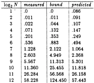
log2N measured bound predicted 1 '.0 .0 .086 2 .011 .011 .091 3 .022 .044 .107 4 .071 .132 .147 5 .201 .353 .249 6 .536 .883 .494 7 1.228 2.122 1.064 8 2.603 4.949 2.368 9 5.567 11.313 5.301 10 11.360 25.455 11.818 11 26.284 56.568 26.158 12 58.228 124.450 57.443

Table 2.1: The maximum magnitude error of the FFT output which is computed using a table of precomputed coefficients. The coefficients are quantized by the 8 bit uniform quantizer. The measured error is listed under the measured column. The analytical bound is listed under the bound column. The error predicted by the empirical formula is listed under the predicted column.

that the calculated bounds are approximately twice the measured values. This suggests that the bound can be scaled to predict the FFT output error. The functional form of the bound and the measured errors are used to derive an empirical formula for the FFT output error. A linear model of the form a A 2 (log2 N - 1) + / is fit to measured data by choosing a and to

minimize the squared error. Thus

N

a A (log2 N - 1) + 3 e measured ije{~ (2.18)

2

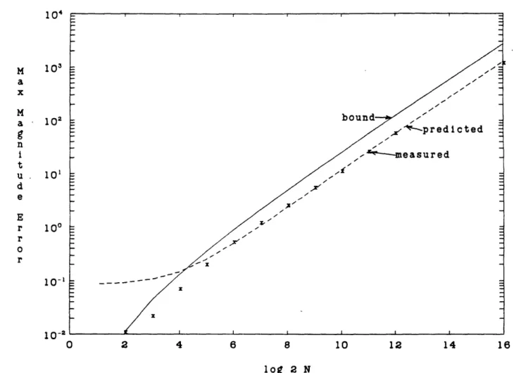
with least squares solution a = 0.65 and / = 0.08. The values in the predicted column on Table 2.1 are computed using the above equation. There is an excellent agreement between the predicted and the measured values. To check the bound for very large N, the error for a 216 length FFT is computed. Because the FFT length is rather large, the search for wo was limited to a small frequency range. The search for the maximum resulted in lelao = 1356.65. The upper bound given by (2.16) is 2715.3 and

j[leloo

is predicted to be 1251.45 by (2.18). Figure 2.1 plots the measured

llelt

, the predicted (2.18), and the bound (2.16) for an 8 bit uniform quantizer. The figure demonstrates that the bound is reasonable and the empirical formula accurately predicts the error.

27

---104 M 103 a x M a

-

102

g

n i t u . 10 d e E r 10 r o r 10-1 I -2 0 2 4 6 8 10 12 14 16 1og_2 N

Figure 2.1: The maximum magnitude error of the FFT output which is com-puted using a table of precomcom-puted coefficients. The coefficients are quantized by the 8 bit uniform quantizer. The measured error, denoted by 'x', the analyt-ical bound, and the empiranalyt-ical formula are plotted.

2.4.2

Probability of Detection using Quantized Coefficients

The FFT output error due to coefficient quantization degrades the probability of detection. The probability of detection at the correct FFT bin is given by (2.9). Because the FFT imple-ments a bank of matched filters, the definitions of both the probability of detection, denoted

PD, and the probability of false alarm, denoted PF, are modified. The detection over all FFT

bins is defined as a decision that a signal exists at the correct bin, k = ko. The false alarm over all FFT bins is defined as a decision that a signal exists at an incorrect bin, k ko, where the

frequency of the signal is wo = ko0.

The quantized-coefficient FFT for input Aew'l"n + w(n) is given by

N-1 _ N-1

(k)-= Ae7WOnWk +

Z

w(n)Wkn

n=O n=O

where WIkn denotes the quantized coefficients shown in (2.12). If the coefficients have no quantization error then ,N-o AeJw'.nWkn = ANS(k- ko). For k

7

ko,

N-l

-| AeUnWo n I < Allelioo.

n=O

The equality is assumed for a conservative D estimation. Therefore, the probability density function of i, where'i = I(k)i, becomes

p(i)= 2 Io(N

_Yo

_{Noa2 ''2Na}

2 Ailejoo)exp(_- +A 2 2

_ll)u()

hence the probability of false alarm over all FFT bins is

PF

i

2

A2=o

Iello

Q(

o

7

P

Na2Io(

2Alleloo) exp(-

Z

)d. = Q(

e'

(2.19)

Na2

2No

2

vW-o '

!

For k = ko,

N-1

I -

AeJwnWJnl > A(N-

Iello)

n=O

Again the equality is assumed for a conservative estimate of PD. Therefore, the probability density function of 2 becomes

___N2

It ll)) ;2(- 2 + A2(N -

Ilel

)2

P(M = N aIo( A(N - Ilelloo)) exp(- -))

Na~_02 -g0 2Na2

29

hence the probability of detection over all FFT bins is

D

j

=f2Io( N 2A(N - lell))expA( -

e

)2

= Q(A(N - ell) 7) (2.20)

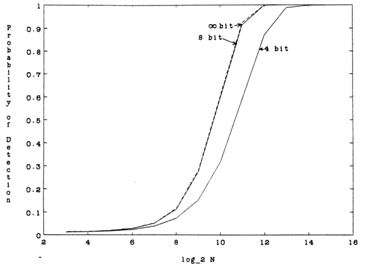
The empirical formula (2.18) is used for [lello in (2.19) and (2.20). Figure 2.2 shows PD as a function of FFT length. It is generated assuming that the amplitude of the sinusoid is 0.1 and the variance of the WGN is 1. The threshold is determined by satisfying the constant false alarm rate of PF = 0.01. Even though the error,

jleioo,

increases as the data length increases, PD also improves. The simulation shows that 8 bit quantization only slightly degrades the probability of detection while 4 bit quantization noticeably degrades the probability of detection. This analysis indicates that it is important to quantize the coefficients using more than 4 bits. In this thesis, the FFTs are computed with coefficients that are quantized using 8 bits or more, so that the degradation in the probability of detection due to the inaccurate coefficients can be ignored.

2.5

Deficiency of Detection Based on a Series of Binary

Hy-pothesis Tests

The receiver operating characteristic of the detector based on a series of single channel binary hypothesis tests as proposed in Section 2.2 is discussed in this section. Assume that the received data have the narrowband component in K of L channels. In this case, the correct output of the detector is the decision that the emitter is absent or, equivalently, that the narrowband component does not exist in all L channels. If the detector decides that the narrowband component exists in all channels, it is a false alarm. Because the proposed detector tests L channels separately, the probability of false alarm is determined by the product of K probabilities of correctly deciding that the channel contains the narrowband component when it does and L - K probabilities of incorrectly deciding that the channel contains the narrowband component when it does not. Therefore, the probability of false alarm, denoted PF,m, is given by

PFm = PF -K X PK

30

1 P 0.9 r o b 0.8 a b i 0.7 1 0.6 0 0.5

r

D 0.4 e V 0.3 I 0.2 n 0.1 A 2 4 6 8 10 12 14 16 log_2 N

Figure 2.2: The probability of detection(PD) of the FFT which is computed with the precomputed table of quantized coefficients. The sinusoidal amplitude(A) is 0.1 and the variance of the WGN(o2) is 1. The false alarm is set to 0.01.

PD for the ideal FFT coefficients, 8 bit uniformly-quantized coefficients, and

4 bit uniformly-quantized coefficients are plotted as a function of the data length(log2 N).

31

--where

PF

and

PD

are the probability of false alarm (2.7) and the probability of detection (2.8)

of the single channel detection, respectively.

The probability of detection, denoted PD,m, is given by

PD,m = PDL.

Because

PF

< PD, PF,m increases as K increases and the detection performance degrades

because PD,m is constant for all K. For the example, let L = 20, PD = 0.95 and

PF

= 0.5,

then the probability of detection PD,m is 0.35 and the probability of false alarm is 1.8 x 10-6

for K = 1, 5.8 x 10

- 4

for K = 10, and 0.19 for K = 19. This confirms that there is a significant

loss in the probability of detection as K increases.

The amplitude of the narrowband component can vary substantially without affecting the

detection performance of the detector based on a series of binary hypothesis tests. Thus, this

method is insensitive to the amplitude variation of the narrowband component and it cannot

enforce the requirement that the amplitude A of A cos(wn + *1) for

= 1, 2,- * , L must be

the same. Additionally, this detector requires many tests and the simple Neyman-Pearson

threshold cannot be used. To remedy these problems, all channels are used simultaneously to

derive detection statistics in the next chapter.

2.6

Summary

In this chapter, the multichannel detection problem was formulated as a series of single

channel binary hypothesis testing problems. Each single channel binary hypothesis testing

problem is solved by threshold testing the Fourier transform magnitude or, equivalently, the

periodogram of the data. The periodograms are computed using the FFT and it was shown

that the quantization of the FFT coefficients has a minimal effect on detection if 8 bits or more

are used for the quantization. The receiver operating characteristic of the single channel binary

hypothesis test was derived and was used to determine the performance of the detector based on

a series of binary hypothesis tests. It was shown that the performance of the detector degrades

noticeably when many channels contain the narrowband component under the Ho hypothesis.

32

Chapter 3

Multichannel Detection Statistics

The performance of the detector based on a series of single channel binary hypothesis tests discussed in Chapter 2 can be improved upon because it does not use data from all channels collectively. In this chapter, both average and semblance, which use data from all channels collectively, are discussed as detection statistics for the multichannel detection problem. As is well known, the average is the generalized likelihood ratio test(GLRT) detection statistic for a particular multichannel detection problem. It will be shown that the average performs well if the received data fit the model of the detection problem. Deviations from the model result in degradation in detection performance. To accommodate the received data for which the average performs poorly, the semblance is introduced and its detection performance is analyzed. It will be shown that the semblance does not perform as well as the average in some important cases. Therefore, to maintain good performance over a wide range of received data, the average and the semblance can be combined to produce a new detection statistic. Combining the average and the semblance is discussed in Chapter 4. This chapter separately analyzes the average and the semblance.

3.1

Average

A multichannel hypothesis testing problem for which the average is the GLRT detection statistic is discussed in this section. Testing the average is identical to testing the sum because any monotonic transformation of a test statistic does not affect the ROC. For convenience, the

33

.-^11111·-

-I1 -··1__-

11111

11 --

- 111_

probability density function of the average is discussed using the sum in this section and the

detection performance of the average will be examined in Section 3.4.

3.1.1

Multichannel Binary Hypothesis Testing Problem

In Section 2.2 the multichannel detection problem was analyzed as a multiple hypothesis

testing problem. In this section, a special case of the multichannel detection problem for which

the average is the likelihood ratio detection statistic is examined. The multichannel detection

problem (2.1) is analyzed by assuming that all channels contain only wideband noise under the

Ho hypothesis and all channels contain the narrowband component in additive noise under the

H

1

hypothesis. The received data model for the composite hypothesis testing, then, becomes

rl S1 + Wl

r

L S + WL

(31)

(3.1)

Ho: R=

I

=

I

where R denotes the received data, L is the number of channels, and N is the number of

samples. As in Section 2.2, the nth sample of the th channel narrowband component vector,

s, is s(n) = A cos(wLn + 01) where A, w, and 01 are unknown parameters. The nth sample of

the Ith channel noise vector, w, is wl(n) and the wl(n)'s are assumed to be white Gaussian

noise as a function of I and n with zero mean and a

2

variance. The above received data model

for the Ho hypothesis does not contain the narrowband component, therefore, it is simpler than

the model employed in Section 2.2.

The multichannel detection problem (3.1) with unknown parameters is solved using the

GLRT by replacing the unknowns with the ML estimates. The GLRT solution for this detection

problem is given by a vector form of (2.2) as

maxAO w PRIH, ,A, , (RJ H1, A,

m,

o) H,

Ag(R) = PIHo(RIH )o 0 (3.2)

pIH(RIHo

)

HO

where the received data is R = (1r,r2,- ,rL)

T

with r = (ri(O),ri(1l),

..

,rl(N - 1))T, w =

(4W,w2, ,WL)T, and =

(l,

, qL})T2,' T. The threshold value r7o is set to match a specified 34