Developing an Integrated Rail Simulator for SimMobility
byKenneth Hang Chang Koh B.Sc Mechanical Engineering
University of Illinois at Urbana-Champaign, 2015
Submitted to the Department of Civil and Environmental Engineering in partial fulfillment of the requirements of the degree of
Master of Science in Transportation at the
MASSACHUSETTS INSTITUTE OF TECHNOLOGY June 2017
@2017 Kenneth H.C. Koh. All rights reserved.
The author hereby grants to MIT permission to reproduce and to distribute publicly paper and electronic copies of this thesis document in whole or in part in any medium now known or hereafter created.
Signature redacted
A u th o r... ... ...
Department of Civil and Environmental Engineering
d
June 19, 2017
Signature redacted
Certified by... ...
Moshe E. Ben-Akiva
/
/ Professor of Civil and Environmental EngineeringCertified by.
Signature redacted
Thesis Supervisor
Accepted by...
Signature redacted
MASSACHUSETTS INSTITUTE OF TECHNOLOGY
JUN 14 2017
Professor of C
Carlos Lima Azevedo Research Scientist Thesis Co-Supervisor ...
Jesse Kroll
Civil and Environmental Engineering hair, Graduate Program Committee
77 Massachusetts Avenue
Cambridge, MA 02139
MIT~ibranes
http://Iibraries.mit.edu/askDISCLAIMER NOTICE
Due to the condition of the original material, there are unavoidable
flaws in this reproduction. We have made every effort possible to
provide you with the best copy available.
Thank you.
The images contained in this document are of the
best quality available.
Developing an Integrated Rail Simulator for SimMobility
byKenneth Hang Chang Koh
Submitted to the Department of Civil and Environmental Engineering on June 19, 2017 in Partial Fulfillment of the Requirements of the Degree of Master of Science in Transportation
Abstract
High-frequency rail transit systems such as subways play a key role in urban transportation; as such, the choices made in the design, implementation, and operation of rail networks are important. To fully understand the impacts of these choices, there is a need for an integrated analysis, where the rail system is analyzed as a component of a larger transportation network. This thesis focuses on designing a
rail simulator as an integrated component of the SimMobility simulation platform, improving upon existing simulators via complete integration with the comprehensive features of SimMobility, enabling it to account for multimodal demand by dynamically adapting to changes in the entire network. A second aim is flexibility; through the implementation of a Service Controller able to read user-written LUA files,
it is shown that the rail simulator is able to model a wide variety of different scenarios and policies. The rail simulator is then calibrated using a novel sequential calibration method, where individual
parameters are estimated sequentially. The advantage of this method is its computational speed and ability to operate with only automatic fare card (AFC) data, not requiring automatic train control (ATC) data. This approach is shown to result in a 30% error in travel times, making it an ideal first-step approach to generate seed values that can be used for more comprehensive calibration methods.
Finally, the rail simulator is used to conduct a historical disruption scenario and investigate the effects of a simple mitigating strategy. The effects of the various scenarios on not only the rail network, but also the road network and passenger welfare, are captured, thus demonstrating the usefulness of an
integrated simulator in research and future planning. Thesis Supervisor: Moshe E. Ben-Akiva
Acknowledgements
I would firstly like to thank my advisor, Prof. Moshe Ben-Akiva, for the assistance and guidance he has
given me over the course of my studies at MIT. The rigorous, yet fair academic standards he imposes on his students have been an inspiration to me; furthermore, he has also been a pillar of support both academically and psychologically. I am honored to have had the opportunity to work with him. I would also like to thank my thesis co-supervisor, Dr. Carlos Azevedo, for the tremendous help he has provided over these past two years. Always approachable, his uncanny ability to identify potential problems in my research, and suggest solutions to them before they even occur, has improved the quality of my research and this thesis immeasurably.This research would not have been possible without the contributions of the researchers at SMART, who transformed the models and concepts described in this thesis into a working simulator. I am especially grateful to Kakali Basak, Zhang Huai Peng, and Jabir Karachiwala for the amazing work they have done in coding, fixing bugs, and generally making sure that everything functioned properly.
I am also indebted to the Land Transport Authority of Singapore for providing me with the financial and administrative support necessary to pursue my graduate studies at MIT. I would like to especially thank Jeremy Wong, who has efficiently helped me with various administrative matters over the course of the past four years.
To my friends in MIT, other parts of the US, or back in Singapore, thank you for the emotional and social support. Studying can be an exhausting affair, and I appreciate all the laughter, companionship, and conversations that distracted me from the stress of research and made this time more bearable. To Augustine, Auriga, Clement, Jon, and everyone else (you know who you are), thank you for helping me keep my sanity, especially (unfortunately?) during final exam week every semester.
Last, but definitely not least, I would like to thank my family: my sister, for being a constantly humorous, yet encouraging, presence in my life, and my parents, for their continuous, unwavering encouragement and support. I would not be here today, on the cusp of graduating from MIT, without their love, nor the sacrifices they have made over the past 25 years of my life. This thesis is dedicated to them.
Table of Contents
CHAPTER 1: INTRODUCTION ... 9
1.1 M otivation...9
1.2 Types of Sim ulation M odels... 12
1.2.1 M icroscopic ... 12
1.2.2 M acroscopic...12
1.2.3 M esoscopic ... 13
1.2.4 Tim e- vs. Event-Based Sim ulation ... 13
1.3 Literature Review ... 14
1.4 Research Approach ... 20
1.4.1 W hy Choose Sim M obility. ... 21
1.4.2 W hy Sequential Calibration?... 21
1.4.3 Thesis Outline... 22
CHAPTER 2: DEVELOPING THE RAIL SIM ULATOR ... 23
2.1 Overview ... 23
2.2 Fram ew ork and Com ponents ... 24
2.3 Active and
Inactive
Pools ... 312.4 Train M ovem ent & Signaling...34
2.4.1 Overview of Signaling Principles ... 34
2.4.1.1 Fixed-Block Signaling... 34
2.4.1.2 M oving-Block Signaling ... 35
2.4.1.3 Design Considerations... 35
2.4.2 Signaling and Train M ovem ent Fram ew ork... 36
2.4.2.1: Start of Tim e-Step ... 37
2.4.2.2 Updating Variables for Subsequent Tim e-Step... 39
2.4.2.3 Potential
Issues
... 402.5 Passenger-Train Interaction: Station M odels ... 41
2.5.1 Overview of Station Behavior ... 41
2.5.2 Calculating Dw ell Tim e ... 42
2.6 The Service Controller...44
CHAPTER 3: CALIBRATION...47
3.2 The Case Study ... 48
3.3 Data Structure ... 49
3.4 Estim ating Train Speeds... 51
3.5 Estim ating W a it Tim es ... 53
3.6 Estim ating W alking Tim es ... 54
3.7 Estim ating Dw ell Tim es... 57
3.7.1 Preparing the Data Set ... 58
3.7.1.1 Pruning the Data Set ... 58
3.7.1.2 Scaling the Data Set ... 59
3.7.2 Perform ing Iterative Estim ation... 62
3.7.3 Results... 63
CHAPTER 4: VALIDATION ... 67
4.1 Validating Calibration Param eters ... 67
4.2 Disruption Scenarios ... 70
4.2.1 Introduction ... 70
4.2.2 Results...71
Chapter 5: Sum m ary and Future W ork...74
5.1 Sum m ary ... 74
5.2 Recom m endations for Future W ork ... 75
5.2.1 Expanding the Scope...75
5.2.2 Im proving Accuracy in Estim ation ... 76
5.3.3 Future Case Studies...78
Appendices...80
Appendix 1: List of Im plem ented APIs... 80
Appendix 2: LUA code for Disruption ... 86
Appendix 3: Singapore North-East Line Operating Specifics ... 90
Bibliography ... 91
List of Figures
Figure 2.1: Structure of the SimMobility Mid-Term Simulator... 23
Figure 2.2: Entities in the North-East Line ... 25
Figure 2.3: Passenger Flow in the Rail Simulator... 29
Figure 2.4: Train Flow in the Rail Simulator ... 30
Figure 2.5: Active & Inactive Pools... 32
Figure 2.6: Fixed-Block Signaling... 34
Figure 2.7: Simulated Speed-Time Profile... 36
Figure 2.8: Defining Train Movement Variables ... 37
Figure 2.9: Approaching Station Decision Logic... 42
Figure 3.1: Singapore Rail Network ... 48
Figure 3.2: Speed-Time Profile of NEL Train ... 51
Figure 3.3: Marymount to Chinatown Route Choice Estimation ... 60
Figure 3.4: CDFs of Simulated vs. Actual Travel Times ... 64
Figure 3.5: Comparing Simulated and Actual Travel Times ... 65
Figure 4.1: Heatmaps of Calibration Demand vs. Validation Demand ... 67
Figure 4.2 Validating CDFs of Simulated vs. Actual Travel Times ... 69
List of Tables
Table 2.1: Attributes of Agents and Entities in the Rail Sim ulator ... 27
Table 2.2: Decisions M ade by Agents and Service Controller... 27
Table 3.1: Effective M aximum Speeds on the NEL ... 52
Table 3.2: Station W alking Time Coefficients ... 56
Table 3.3: Scaling Table for NEL-Partial Trips... 61
Table 3.4: Estim ated Dwell Time Parameters... 63
Table 4.1: Sum mary of Disruption Scenario Results... 72
Table 4.2: M ode Share in Disruption Scenarios... 73
CHAPTER 1: INTRODUCTION
1.1 Motivation
High-frequency rail transit systems play a key role in urban transportation, transporting large volumes of commuters from origin to destination daily and significantly alleviating stress on the road network. Indeed, more than 50% of residents in major population-dense cities such as Hong Kong, Singapore, Tokyo, and London, rely on public transport for their daily commute (Di, 2013)7. As such, the choices made in the design, implementation, and operation of rail networks are of considerable importance. To understand the impacts of these choices, there is a need to perform an integrated analysis-considering not only effects on the rail network, but the resulting effects on future demand and the transportation network as a whole-when designing and assessing potential rail systems, or proposed modifications to existing systems. Similarly, there is a need to examine both normal operating conditions, and system disruptions, with the latter typically being harder to study given its short analysis period and the detail required to analyze system performance and traveler reactions.
A natural approach to this analysis is through simulations, which allow for the examination of a
multitude of scenarios that would be too expensive or impractical to conduct in the real world. In an ideal world, we would be able to capture every relevant variable and their interactions, and yield a perfect picture of the real-world effects of theoretical disruptions; of course, this is unfortunately beyond the capabilities of anything humanly possible today. A more realistic option is to design a simulator detailed enough to represent important interactions, yet streamlined enough to be computationally efficient, and flexible enough to simulate a range of varying scenarios.
More importantly, it is necessary to design an integrated rail simulator that captures not only demand and supply interactions within the rail network, but also how these interactions affect other modes of transport, and how a commuter's experience in one day affects his decisions in the next. After all, this
interplay of variables is a basic tenet of real-world transportation decisions-for example, if a commuter
consistently experiences train delays, he might lose faith in the system and simply start taking the bus-and to ignore it in the simulator would result in an incomplete model bus-and limited understbus-anding of cause-and-effect.
Such an integrated rail simulator should, via interfacing with other simulators and an overarching framework, be able to account for multimodal demand. Passenger demand should affect system performance; similarly, changes in system performance should feedback and affect future passenger demand, resulting in a clear picture of overall transportation choices. It should also be extremely flexible, able to mimic the real world by simulating a large array of scenarios.
However, the undeniable usefulness of advanced, integrated simulators gives rise to a secondary problem; that of calibration. The models used in these simulators are, by virtue of their complexity, typically data-eager, and require tremendous amounts of data and computational power to produce accurate and reliable results.
Calibration of supply has typically been done by simply utilizing historical data, or manually collecting data at certain stations, then extrapolating and generalizing this data to the entire train network.
However, the former is insufficient for an integrated simulator, which demands information for which historical data may not exist (such as walking times within stations) or may be inappropriate (such as dwell times, which should vary dynamically with demand and not simply be a historical average). The latter, on the other hand, tends to be extremely labor intensive and requires the use of significant assumptions (for example, that the properties of one station represent the properties of all stations on a line). These methods therefore lead to inaccuracies and are counterproductive to the goal of developing an advanced simulator.
A potential solution to this lies in the use of electronically recorded data. In recent years, due to rapid advances in communications technology and the increasing ubiquity of electronic devices, automatic
fare collection (AFC) via the use of smart cards (or even phones in some cities) is being adopted by an increasing number of transit agencies worldwide. Such a method offers many advantages: not only is it a convenient, straightforward, and secure method of paying fares, it also allows the operator much more flexibility in implementing specialized fare schemes. Along with this proliferation of electronic fare collection comes a wealth of data: a detailed log of journeys made by commuters over time. Analysis of this data may yield insights into a wide array of transportation issues such as commuter behavior, response to new policies and so on. However, there is a significant drawback: commuters' movements while they are within the system are not tracked (that is, most systems only record at point-of-entry and, occasionally, point-of-exit). Hence, this data has often been used with train movement data (known as automatic train control, or ATC) to match passengers to trains and therefore calibrate supply. This,
unfortunately, poses a problem in cases where ATC data is unavailable-which, due to privacy concerns, is becoming more prevalent.
This thesis proposes a solution to this problem via the method of sequential calibration to calibrate the supply of trains in a rail simulator. In this method, AFC data is used together with General Transit Feed Specification (GTFS) data and minimal manual data collection to calibrate many aspects of train supply. The goal is to utilize certain assumptions to bypass the need for ATC data, thus yielding reasonably accurate estimations of key parameters quickly.
This thesis is divided into five main parts. Chapter 1 provides an overview of the existing literature, and defines terms that will be used in this thesis. Chapter 2 focuses on the development of a rail simulator as part of the state-of-the-art SimMobility simulation platform. It presents the overall structure and design of the simulator, and demonstrates how the unique addition of the Service Controller allows the simulator to be extremely flexible. Chapter 3 focuses on the calibration of the rail simulator, and
presents the method of sequential calibration as an alternative to calibrate train supply models where data is sparse. Chapter 4 focuses first on the validation of the parameters estimated in Chapter 3, and
subsequently on the validation of the rail simulator developed in Chapter 2 by comparing simulated disruptions with historical disruptions on the Singapore rail network. A simple disruption management solution is then proposed and implemented to demonstrate the capabilities of the rail simulator.
1.2 Types of Simulation Models
In the interests of clarity, it is necessary at this point to briefly digress and describe the various types of commonly used simulation models, as these terms will be used to evaluate existing simulators in the next section. There are three main types of models, microscopic, macroscopic, and mesoscopic, and two main types of simulators, time-based and event-based. The distinction between these choices lie in the complexity and computational resources required, and each choice can be thought of as representing a certain level of detail.
1.2.1 Microscopic
In a microscopic model, each individual entity in the simulation is explicitly modelled. In the context of a train simulator, each train and passenger is modelled explicitly, and system properties such as dwell time are determined through passenger/train behavior models that replicate the decisions made by individual passengers when boarding or alighting. Microscopic models tend to provide the most accurate simulations, but require significant computational power.
1.2.2 Macroscopic
In a macroscopic model, entities are aggregated together and not modelled individually. For example, a train simulator could simply track the number of passengers in the system, instead of modelling each
passenger individually, and determine system properties such as dwell time via a function of the number of boarding passengers, alighting passengers, and overall crowdedness of the train. Macroscopic models are often orders of magnitude quicker than microscopic models, and require less information about the system, but sacrifice accuracy.
1.2.3 Mesoscopic
In a mesoscopic model, entities are implemented using both aggregated and disaggregated models. For example, the train simulator in this thesis models passengers' walking times within a station individually, but determines dwell time as a function of passenger volume to reduce computational costs.
Mesoscopic models can be thought of as a "middle ground" between microscopic and mesoscopic models, with key areas simulated microscopically and the rest simulated macroscopically.
1.2.4 Time- vs. Event-Based Simulation
In time-based simulation models, the simulation is divided into evenly-spaced intervals. At each interval, the current state of the system is evaluated and the behavior of entities within the system is calculated for the next interval. As such, the system evolves continuously over time, and is conceptually similar to what occurs in reality. However, such a model usually requires significant computational power to generate the information required at every time-step.
In contrast, in event-based simulation models, the simulation progresses via the occurrence of a sequence of pre-defined events. When an event occurs (for example, a passenger arrives at the station),
all variables relevant to that event are updated and the time of the next event calculated. As such, the simulation progresses at irregular intervals, and the updating of variables occurs asynchronously, resulting in information on the state of the system between events often being hazy. However, this approach substantially reduces computational effort and yields quick results.
Ultimately, the decision of what type of model to develop is primarily a decision on the trade-offs between accuracy and computational speed. In the integrated, multimodal rail simulator that this thesis aims to develop, time-based simulation is crucial. Given that events that occur in one simulator may affect events in another simulator, an event-based model is an inelegant approach; furthermore, given the constant feedback between supply and demand, a time-based simulation allows passengers to
instantly react to the current state of the system, and is ideal for capturing the performance of a transportation network in reality.
1.3 Literature Review
There is a reasonable amount of prior work involving the development of train simulators to investigate various problems such as train scheduling, supply, disruption management, and so on. (Goodman et al., 1998)8 provide a helpful framework for categorizing different types of train simulators, and their relative advantages and disadvantages. Their work has been summarized in the preceding section.
Simple macroscopic simulators such as Bahn33
and MetroModSim34 have been developed by
independent parties to provide primarily visual representations of rail networks; in these simulators, trains move at deterministic speeds, with only rudimentary signal controls such as linked pairs of
Stop/Go signals (when one signal says Go, the other signal says Stop, and vice versa). On the other hand, commercial simulators such as OpenTrack (Nash et at., 2004)21, a microscopic time-based railway simulator, provide a comprehensive model of train movement across long distances. However, they tend to not focus on demand-side effects such as dwell time or route choice, and are commonly used in long-distance freight transportation planning instead.
AIMSUN and VISSIM are popular commercial simulation programs used in traffic modelling (Hidas, 2005)1 that place an emphasis on integration, where large-scale mesoscopic simulators interact with more detailed time-based microscopic models to simulate traffic flow and, in the case of the former, even generate demand based on geographical and socioeconomic data. However, these simulators exist primarily to model traffic, with agents in the simulator being vehicles, not passengers; as such, there is a heavy emphasis on multimodal interactions on the road, but a lack of breadthwise integration with other forms of transit, such as dedicated-track rail.
In academia, rail simulators are often developed to investigate various supply-side policies. For example, (Grube et aL., 2011)' and (S nchez-Martinez, 2012)26 both created discrete event-based simulators to increase the operational efficiency of high-frequency rail transit, such as intra-city subways, by
implementing various resource allocation strategies. (Cha et al., 2014)' constructed a similar model for Maglev trains to investigate how varying passenger arrival rates affect system performance. Others utilize rail simulation in operations research, such as to optimize bus-based disruption recovery strategies in subways in Australia (Darmanin et al., 2010)6, Singapore (Jin et al., 2013)14, and so on. However, these models are often customized to the topic at hand and hence over-simplified, only serving as a tool to demonstrate the proposed operational strategy. For example, (Grube et aL., 2011) assume constant speeds and ignore operational restrictions (such as safe distances) between events, while (Ravichandran, 2 0 1 3)2s and (Senchez-Martinez, 2012) utilize historical running time data instead of
actively simulating train movement. (Cha et al., 2014) utilize a linear dwell time based off historical data, and ignore the effects of passenger congestion. (Darmanin et aL., 2010) and (Jin et aL., 2013) only consider deterministic choice (that is, when the subway breaks down, passengers automatically take the substitute bus) and ignore the possibility of individual agents revising their mode or destination choice due to this disruption.
Of course, more complex academic simulators do exist. MATSim is an integrated multimodal simulator
that generates demand from a synthetic population (Horni et aL., 2016)"; however, it also focuses primarily on road transit, with the intricacies of demand-side effects (such as dwell time) notably absent from its embedded rail simulator. Similarly, SUMO3
s is a microscopic time-based multimodal simulator that supports passenger mode choice; however, it lacks dynamic feedback (once a commuter makes a choice, he will not change his mind) and has limited rail simulation capabilities.
SimMobility (Lu et al., 2015)19 is an integrated simulation platform that uses three simulators (Term, Mid-(Term, and Short-Term) to generate an accurate picture of demand and supply. The
Term simulator governs decisions made over months or years (such as house/job location choice), the Mid-Term simulator governs decisions made over hours or minutes (such as route or mode choice), and the Short-Term simulator governs decisions made over seconds (such as path choice). A unique feature of the SimMobility Mid-Term is its publish/subscribe mechanism, where agents modify their travel plans
on-the-fly based on current conditions-for example, a commuter that originally planned to take the
train may choose to drive if the trains are exceptionally crowded. This mechanism is exceptionally useful in simulating disruption scenarios, where commuters often react to imperfect, constantly changing information. However, the SimMobility Mid-Term lacks a dedicated rail simulator-passengers who choose to take the subway are simply moved to their desired destination after a delay corresponding to distance moved. As such, it is unable to capture the nuances of rail transportation, and the effects of changes to the rail system on the overall transportation network.
A common theme of the above simulators is that, within rail transportation, passengers tend to be modelled macroscopically and feedback-reactions to the current state of the system-does not exist. There is therefore a need to develop a simulator where passengers are modelled microscopically, to better capture individual choices and responses to system conditions, as well as impacts that events occurring in the rail system have on the overall transportation network. A second consideration is developing a simulator flexible enough to simulate a wide range of different scenarios, thus reducing the need to custom-develop simulators in the future and eliminating duplication of effort.
Within a train simulator, there are various approaches to modelling aspects of train behavior. When modelling train movement, it is necessary to decide how trains should move between stations, as well as what type of signaling system, if any, should be in place. If train movement is not crucial to the purpose of the simulator, a typical approach as found in Bahn and the simulator developed by (Grube et al., 2011) is to simply assume a constant movement speed. (Kraft, 2013)16 demonstrates that an
and constant deceleration, results in a fairly good approximation to train trajectories in real life. If more detail is required, commercial simulators such as OpenTrack allow for variations in speeds and fuel consumption depending on the tractive power of the engine, track gradient, and track curvature.
However, this comes at the expense of computational cost.
(Chang et al., 1998)' provide a good summary of the differences between the two main types
(fixed-block and moving-(fixed-block) of signaling systems. The former, being an older variant, is more widespread,
but is steadily being replaced by the latter in rail networks worldwide, which allows for trains to operate with significantly reduced headway. (Hill et
al.,
1992)" provide a framework for the implementation of these systems in a rail simulator.Similarly, there are various approaches to modelling dwell time, ranging in complexity. Bahn adopts the simple approach of randomly and uniformly drawing from a pool of prospective dwell times. However, this approach lacks accuracy and is unlikely to mirror real-world conditions. An improved approach is to draw dwell times from a calibrated distribution, based off historical data. This approach is used in various simulators such as the one developed by (S nchez-Martinez, 2012), however, it by default assumes a largely stable demand and is inappropriate to simulate disruptions, where passenger numbers often swell dramatically.
The Maglev simulator in developed by (Cha et al., 2014) utilizes historical data to calculate the mean boarding and alighting time per passenger, which is then multiplied by the total number of alighting and boarding passengers to obtain the dwell time. However, this model relies on the simplifying assumption that dwell times scale linearly with passengers, and ignores congestion-related effects.
(Lin et al., 1992)1" proposed a function for determining dwell time, which was expanded on by (Puong, 2000)24 and shown to be a good fit for the MBTA Red Line. This function depends on train occupancy
and the number of boarding and alighting passengers, and results in the highest degree of accuracy in dwell times across fluctuating demand. This function was adapted for the rail simulator in this thesis.
In many rail simulators such as those developed by (Cha et al., 2014), (Sanchez-Martinez, 2012), (Grube
et al., 2011), amongst others, walking speeds within stations are often ignored, with passengers
assumed to arrive directly at the platform instead of arriving at a fare-gate and then walking within the station to the platform. However, an integrated simulator cannot make this assumption, as the objective
is to consider passenger trips across all modes as a whole, not just the rail component of these trips. Previous work done regarding passenger walking speeds include (Ottomanelli et al., 2012)22 and (Zhang
et al., 2009)"0, who suggest that asymmetric walking speeds are best modelled by a lognormal
distribution. (Zhu, 2014)32 applied this work to train stations and demonstrated that passenger walking speeds within stations followed lognormal distributions as well. As such, this thesis utilizes this
distribution to estimate passenger walking times within the system.
In order to calibrate the various parameters of the simulation, electronic smart card data was used. (Pelletier et al., 2011)23 offer a comprehensive review of the usage of smart card data in various transportation studies. Three categories of studies have been identified: the strategic level, which focuses on long-term planning, the tactical level, which focuses on daily problems such as scheduling, and the operational level, which focuses on the examination of performance indicators such as schedule
adherence. However, at all three levels, the supply is generally already assumed to be calibrated. Smart card data is instead typically used to generate demand-side data which then dictate changes in supply policy. For example, (Zhao et al., 2007)31 present a methodology of using smart card data to generate 0-D matrices for rail passengers.
On the other hand, the calibration of supply is usually done via manual data collection. For example, (Lin
collecting data at two stations during the AM Peak, then generalizing their results across the entire Red Line. While collecting dwell time data at all stations would be labor-intensive to the point of infeasibility, there are nonetheless inaccuracies associated with generating a dwell time function based on
observations from only two stations.
Another common approach to calibrating supply is by simply using recorded historical data (for example, the average dwell time at a station at a certain time of day). This has been done in many simulators such as the one developed by (S nchez-Martinez, 2012), and (Motraghi et al., 2012)20, to name a few, and is a reasonable approach to planning supply-side policy. However, this data may not be readily available and must be collected in some form. Historical data is also unable to predict how a system responds to unexpected changes in demand. Finally, ignoring passenger movements within the stations themselves leads to a lack of accuracy, especially in the case where a passenger uses multiple train lines to complete a trip. It is important to determine how much of this journey time was spent out of transit: walking to a new platform in a transfer station, waiting for new trains, and so on.
In recent years, attempts have been made to utilize electronic data to expedite the calibration process. (Sun et aL., 2015)29 propose an innovative method of combining automatic fare card (AFC) with
automatic train control (ATC) data to match passengers to trains, and therefore efficiently estimate the parameters in the system simultaneously. Although this is an efficient method of supply calibration, it requires two sets of data (AFC and ATC), the latter of which may not always be available due to security concerns.
(Sun et al., 2012)" utilized AFC data exclusively to generate an average walking time, dwell time, and train movement speed for entities in Singapore's rail network. However, in their analysis they assumed that these three values were constant across all stations. In the interests of accuracy, we intend to
expand on this approach by relaxing this assumption and generating functions for each distribution at
every station in the network.
Another similar approach to calibration was utilized by (Antoniou et al., 2015)2, which utilized a
weighted simultaneous perturbation stochastic approximation algorithm to simultaneously calibrate all supply and demand parameters for traffic simulation models. Although such an approach is more comprehensive and robust, it can be time-consuming and computationally taxing. In this thesis, we propose that a sequential calibration framework, which requires significantly less computational power, is an effective approach to calibrating rail systems.
Finally, when evaluating the performance of a system under disruption, we consider two main performance metrics, capacity reliability and travel time reliability, as suggested in (Carrion et al., 2012)3. The former refers to the probability that the system accommodates a certain level of demand, while the latter refers to the probability that the system allows commuters to reach their destination within a given timeframe. By evaluating these metrics, we will demonstrate that the rail simulator in this thesis has the capability to evaluate the negative effects of disruptions and the usefulness of proposed mitigation strategies.
1.4 Research Approach
To summarize the discussion in the previous sections, the goal of this thesis is to develop a
comprehensive rail simulator within a multimodal agent-based simulation framework for the analysis of different operational designs. In order to provide a clear picture of supply and demand, generate a feedback loop where commuters react to the current state of the system and vice versa, and enable integration in the form of constant passenger flow between the rail simulator and other transit
be individually simulated for ease of integration, their effects on each other (such boarding/alighting behavior or walking speeds) can be simulated macroscopically.
1.4.1 Why Choose SimMobility?
Given the aforementioned aims, the SimMobility Mid-Term is an ideal overarching simulation platform to integrate the proposed rail simulator with. The Mid-Term already contains many key functions, such as organic demand (obtained from the Long-Term), mode/route choice models and a functioning traffic simulator, which allow for breadthwise integration of the rail simulator to other forms of transit, and the
publish/subscribe mechanism, allowing for the development of a feedback loop between the rail system
and passengers' decisions. Finally, the "blank slate" of the Mid-Term enables the rail simulator to be developed in a similarly flexible manner, allows it to easily simulate a wide range of scenarios (not just disruptions) under a wide array of operating conditions.
1.4.2 Why Sequential Calibration?
After the rail simulator is developed, it should be tested, and this thesis aims to apply it to a case study of a disruption in Singapore. However, due to the difficulties in obtaining ATC data, a few issues arise; firstly, the question of whether the simulator can be efficiently calibrated through AFC data alone, and secondly, the increasing importance of developing an efficient calibration methodology that can be applied to a variety of rail systems in different cities. As such, there are two tenets to the calibration philosophy:
1) The calibration process should rely solely on AFC data as much as possible, as obtaining additional data may be difficult depending on the transit agency in question;
2) The calibration process should minimize the need for manual data collection, in the interests of expediency and as an improvement over current methods.
The sequential calibration process satisfies both these tenets, relying almost exclusively on AFC data to generate reasonably accurate estimations of simulation parameters, and as such is an appropriate choice to calibrate the rail simulator.
1.4.3 Thesis Outline
In Chapter 2, we discuss in depth the design of the rail simulator, using the Singapore subway system as an example. We elaborate on train movement, dwell time, end-of-line behavior, and introduce the Service Controller and explain its function in making the rail simulator extremely flexible.
In Chapter 3, we discuss the calibration of the rail simulator, once again using the Singapore network as an example. We present the framework of sequential calibration, and demonstrate how iterative simulations can be used to calibrate many variables using just AFC data.
In Chapter 4, we present a validation of the methods used in Chapter 3, where the estimated parameters were used to estimate travel times for a fresh day. We demonstrate that the sequential calibration approach is valid, and subsequently apply the simulator a to case study, simulating a real-life subway disruption that occurred in Singapore in 2013. We show that the simulator comprehensively simulates the effects of a rail service disruption and can be used to investigate in detail the effects of
different mitigation policies.
Finally, in Chapter 5, we summarize our findings and offer suggestions for future research. We discuss improvements to the calibration process and disruption simulation, and present suggestions for adapting the simulator to rail networks with different properties in the future.
CHAPTER 2: DEVELOPING THE RAIL SIMULATOR
2.1 Overview
The SimMobility Mid-Term simulator is a time-based mesoscopic simulator integrated both upward (with the Long-Term, which provides population and land use data and the resulting demand) and downward (with the Short-Term, which models minutiae such as path choice). The Mid-Term simulator is itself composed of multiple modules, which work in coherence to provide a clear picture of
individuals' trip, route, and mode choices throughout the course of a day. The interaction between these modules is summarized in (Lu et
al.,
2015) and reproduced in Figure 2.1 below:Population &
Land-use
Pre-daya
Activity schedules
s Trajectories
Figure 2.1: Structure of the SimMobility Mid-Term Simulator
A synthetic population is generated in the Long-Term simulator and passed to the Mid-Term simulator. In the pre-day module, individuals plan their trips and choose routes and modes, based on prior
experiences and current needs. These schedules are then passed to the within-day module, which works in tandem with the supp/y-comprising the road simulator and rail simulator-to generate travel times for each trip. At the same time, the supply simulators constantly provide feedback about their current
performance, which may cause commuters to modify their schedules accordingly. For example, if a commuter becomes aware that the rail network along his desired route is congested, he may instead decide to take a taxi to his destination. As such, there is a constant dynamic interaction between the
within-day and supply modules. Finally, as the day concludes, individuals "learn" from their experiences
and modify their choices in the subsequent pre-day module accordingly. For more information, please refer to (Lu et al., 2015) and (Adnan et al., 2016)1.
In order to interact with the dynamic demand from the Mid-Term simulator, the rail simulator was developed as a mesoscopic simulator, with demand and supply (that is, passenger-Agents and train-Agents) modelled individually, but performance effects (that is, the effects of passengers on dwell time) modelled at an aggregate level. The rail simulator itself is comprised of Agents and Entities, which are both modelled microscopically, with individual Agents/Entities having unique associated parameters. The key distinction between the two terms is that Agents are vested with decision-making abilities, while Entities make no decisions whatsoever. These are both regulated by an overarching Service Controller, which constantly evaluates the current state of the system and dynamically defines certain targets for Agents, such as speed limits or dwell times for train-Agents, or walking times for passenger-Agents. Finally, the user manipulates this Service Controller through the use of APIs to simulate various conditions and scenarios.
2.2 Framework and Components
In this section, we will provide a general overview of the infrastructure models and frameworks for passenger and train movement used in the rail simulator. The subsequent sections in this chapter will further elaborate on the models used in these frameworks, namely train pools (depot modelling), train
movement models (speed and acceleration modelling), passenger-train interaction models (dwell time
Before proceeding, it is necessary to define key terms in the proposed rail simulator. A pool is analogous to an "uninvolved area" (a depot, sidings, etc.), and represents an area where out-of-service trains wait (this will be further elaborated in Section 2.2). A platform corresponds to a specific train service in a specific direction, and is irrelevant to the number of physical platforms a station has. As such, most stations contain two platforms, with interchange stations containing more. A station represents a point of connection between the overall Mid-Term simulator to the rail simulator, where commuters are "passed" from the former to the latter. Each station has a unique name as an identifier, shared across all lines the station contains. A block represents a specific section of track with unique properties, and connects platforms to each other. A line represents a sequence of platforms and blocks that trains progress through sequentially during service. As such, train services are effectively represented as two different lines in the rail simulator. Finally, every train is assigned a schedule, which represents an ordered subset of platforms within a line that a train should serve. For example, in Singapore, the North-East Line (NEL) consists of 16 stations, NEI through NE17 (less NE2), and is represented in the rail simulator as two lines: NE_1 consists of the ordered set of platforms {NE1_1, NE3_1, ... , NE17_1} and NE_2 consists of the ordered set {NE17_2, NE16_2, ... , NEl_2}. An express train on line NE_1 could conceivably have the schedule {NE1_1, NE3_1, NE6_1, NE12_1, NE17_1}, which only consists of interchange stations. Figure 2.2 shows a graphical depiction of the first 2 stations on the NEL:
Block I Block 2 B:ck3 Block 4 Block 5
P~atkornNE -ULne NE 1 PiatfotynNF 3
-Pools Station NEI Stafon NE3
I
* eftmPIE 4-2- - -ine NE_2 Pieftcm NE3Block n Block n + 1 Block n + 2 Block n + 3 Block n + 4
The rail simulator itself consists of components which are either Entities, or Agents. The former make no decisions, but have associated attributes that affect decisions made by the latter. Pools, blocks, stations, and platforms are Entities; for example, a station-Entity has walking time parameters that passenger-Agents use to determine their walking time within the station. Block-Entities have acceleration rates and
maximum speeds associated with them that affect how fast train-Agents decide to move on that
particular block-Entity; similarly, platform-Entities have minimum dwell times and maximum dwell times that affect how long trains decide to dwell at the platform-Entity. On the other hand, passengers and trains are Agents; they constantly make decisions based on their own associated attributes, relevant Entity attributes, and instructions from the Service Controller.
More specifically, the Service Controller regulates Agent behavior via the use of internal functions that ensure smooth operation of the system. For example, the Service Controller may impose a second speed limit on a train, in addition to the speed limit already defined by the block-Entity the train is on, to keep two trains a safe distance from each other. Agents are individualistic, only focusing on their current situation; the Service Controller rectifies this by focusing on the system in its entirety.
Finally, the user has ultimate control over the rail simulator. Through the use of application
programming interfaces (APIs), the user is able to interact with the Service Controller to create scenarios worthy of investigation. For example, the user may specify unconventional operating logic, or introduce atypical train behavior such as break-downs, to explore the sensitivity of the system to deviations from standard operation, the robustness of proposed policies, and so on.
Table 2.1 summarizes the various components of the proposed rail simulator and their associated attributes, while Table 2.2 summarizes the decisions made by the Agents and Service Controller.
Pool Entity 0 Pool ID
* Maximum Capacity
* Train Occupancy List (list of Train IDs currently in the pool) * Type (Active/Inactive)
* Dispatch Schedule
Block Entity * Block ID
* Maximum Acceleration/Deceleration Rate 0 Maximum Speed
0 Location * Length
Station Entity * Station ID
* Walking Time Parameters
0 Traits (U-turn, Bypass, Interchange, Shared Track) 0 Maximum Capacity
0 Occupancy List (list of Passenger IDs currently in the station)
Platform Entity * Platform ID
* Dwell Time Parameters 0 Maximum Capacity
* Occupancy List (list of Passenger IDs currently at the platform)
Passenger Agent 0 PassengerlD
0 O-D Path (temporally ordered list of platforms to board, transfer, alight from trains)
* Walking Speed Parameter
Train Agent 0 Train ID
0 Schedule ID
0 Occupancy List (list of Passenger IDs currently in the train) * Schedule
* Length
Table 2.1: Attributes of Agents and Entities in the Rail Simulator
Name Type Decisions
Passenger Agent * Walking Time (within a station)
Train Agent 0 Dwell Time
* Speed
* Acceleration/Deceleration Rate
Service - * Denying Access to Station
Controller * Denying Access to Platform
0 Denying Access to Train
Ultimately, the goal of the rail simulator is to take input from the SimMobility Mid-Term and return output in the form of travel time and associated metrics. In the Mid-Term, passengers are Agents as well, with daily activity schedules, trips, mode choices, and route choices generated by the Pre-Day module, and a "state" corresponding to their current action. When the rail-mode portion of a trip commences, the passenger-Agent's state changes to <<in the rail system>>; at this moment, he is "passed" to the rail simulator, and is hence visible to it. The exact location of this individual in the rail system is then calculated and updated at every time-step until he leaves the rail system; at this juncture, his corresponding state changes, he is "passed" back to the Mid-Term, and is no longer visible to the rail simulator. The individual's total travel time is also returned to the overall Mid-Term simulator, as well as performance metrics such as capacity reliability and travel time reliability.
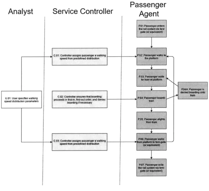
Figures 2.3 and 2.4 below describe the flow of passenger-Agents and train-Agents in the rail simulator respectively. Each step is marked with a letter-number code that denotes whether it is an action taken by the passenger-Agent (P), train-Agent (V), Service Controller (C), or User (U), and its position in the sequence of events.
Passenger
Analyst
Service Controller
Agent
Po1 Passengerenters
Iha fil syatem via tat'
g ate 0or e qurvalent)
C.01: Controget assigns passenger a wanIng P,02: Passenger walks1o speed from predehned distributon the platfarm
P03assenger waits
or tram at platform
U.O1: Usar specties wa~ng C-02 Controler ensurw that boarding
speed distribuion parameters proceds in rt-in, st-oul rde, and denies
P t5- Passnger alghts
Tiam tramn
[*(of
eqwiva IentP07 Passenger exits
the ,raif Sytam Wa fare-gate or equwalent)
P04A Passenger is
denmed board ng onto
t i n
Figure 2.3: Passenger Flow in the Rail Simulator
It can be observed that passenger flow is essentially linear, consisting of 7 steps with minimal
intervention from the Service Controller. The passenger agent officially enters the system (P.01) when it is passed from the overarching Mid-Term simulator to the rail simulator. This typically occurs when the passenger "taps-in" at a fare gate. He then decides his walking time to the platform, based on the attributes of the station he enters at and his own walking speed (P.02, C.01, U.01). The passenger queues in first-in, first-out (FIFO) order and is assumed to board the first train that arrives with sufficient capacity (P.03, P.04, C.02). If a train does not have sufficient capacity, the passenger is denied boarding
(P.03A), and has to wait for the subsequent train. Once boarded, the passenger-Agent "sleeps", with all
movement between stations controlled by the train-Agent. The passenger is then "awoken" at his desired destination (P.05), and decides a walking time to the fare-gate (if exiting the system) or the next
platform (if performing a transfer) (P.06, C.03, U.01). Note that the walking times in P.02 and P.06 are drawn from the same percentile of different distributions to maintain consistency in passenger walking speeds and keep the geometric features of the stations constant. Once the passenger exits the system
(P.07), the train trip is determined to be complete and output is returned to the Mid-Term simulator. This will be further elaborated on in Chapter 3 as a key part of the calibration process.
Analyst
Service Controller
Train Agent
V,30 Tramn rmea es to
02 Cntoer srio a V2 a scedW
I ,t
tLO. LA 0:
~C
~V0
Tai pas anServes Staton
C, 03: C *nftF0Je e-Val UateS M e Current Sraft Of
hthe syslem and any LUA msructions then4 p
nstucs ubequntagntbehavo
V 05: Tramn movps to next _ 4 calon
V05 Tramn rsetLrms W atve Poo1
C4 Controller assigns train anewsthedule OR retires it active pool
In contrast to passenger flow, it can be observed that the flow of trains is significantly more complicated. Service begins when a train is pulled from the inactive pool to the active pool by the Service Controller (V.01, C.01). The former is analogous to a train depot, while the latter is analogous to an out-of-service train waiting at a terminal station. The train then receives schedule information comprising its departure time from the first station, as well as a list of stations to service and its expected arrival time at those stations (V.02, C.02). When a train arrives at a station, it relays this information to the Service Controller, which checks for any especial instructions for the train from the user (U.01). If there are none, the Service Controller boards and alights passengers, calculates a dwell time for the train based on dwell time models, and instructs its subsequent behavior (V.03, C.03).
Similarly, as the train moves between stations, its relative position to other trains and stations in the line is constantly monitored by the Service Controller, and its speed adjusted accordingly subject to the train movement models and especial instructions from the user, if any (V.04, C.03, U.01). Finally, when the train reaches the end of the line, it conveys this information to the Service Controller, which typically assigns the train a new schedule-usually the corresponding return route (V.05, C.04). In rare cases, the Service Controller will instead retire the train from the active pool (V.06, C.04), essentially sending it back to the depot. This occurs when the desired arrival frequency decreases-for example, when the system changes from peak scheduling to off-peak scheduling.
In the subsequent sections, we will elaborate on the implementation of the train flow diagram, starting with the active/inactive pool system, followed by station behavior, movement and signaling, and finally the Service Controller.
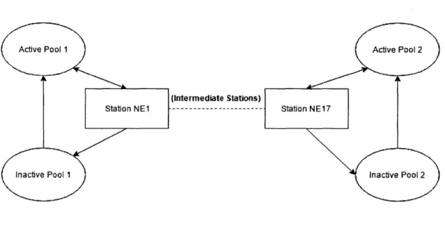
2.3 Active and Inactive Pools
A typical rail system is likely to contain multiple types of trains running at once, each with different properties-for example, older trains are likely to have a slower acceleration rate and maximum speed.
In some cases, trains may differ in length and passenger capacities as well, amongst other properties. As such, it is important to distinguish between individual trains, by assigning each train an ID.
It is also important to distinguish between different states of a train. A train may be in active service (moving along the line and ferrying passengers); however, it may also be waiting (idle at a terminal station or side-track waiting for its next schedule to begin), or out-of-service (that is, at rest in the
depot). The key difference between the latter two states is the effect they have on the system. Trains that are "waiting" are still occupying physical space in the rail network, and can be called into service very quickly. On the other hand, trains that are out-of-service occupy no space-depots are assumed to
have infinite capacity-but take a while to enter service.
This distinction is simulated by having an "active pool" and "inactive pool" at each end of the line. We use the NEL, which has 28 trains total, as an example in Figure 2.5 below. The arrows represent
acceptable directions of movement between the end stations, active pools, and inactive pools:
Active Pool 1 Active Pool 2
(intermediate Stations)
Station NEI --- Station NE17
Fnactive
Pool 1 Inactive Pool 2
Suppose that, during the AM Peak, the NEL has 20 trains in-service and 8 trains out-of-service. When the simulation is initialized, the distribution and order of trains is read from the database. For example, in the NEL trains are evenly distributed amongst both lines NE1 and NE2 and order simply corresponds to Train ID. As such, the simulation initializes with 10 trains (with IDs 1 to 10) in Active Pool 1, 10 trains (with IDs 15 to 24) in Active Pool 2, 4 trains (with IDs 11 to 14) in Inactive Pool 1, and 4 trains (with IDs 25 to 28) in Inactive Pool 2. (Naturally, the number of trains in each pool and their corresponding IDs
may differ for other lines.) As the simulation runs, trains are drawn from in order AP1 and AP2 whenever a new train is dispatched from the end stations (NE1 and NE17 respectively).
When a train reaches the opposite end station from the one it departed, it by default joins the back of the queue in the active pool. Hence, for example, when Train 1 reaches NE17, it queues in Active Pool 2
behind Train 24. However, the Service Controller may alter this behavior if predefined conditions are met (for example, if the AM Peak is about to end and less trains are required in service), or if the user specifies contrary instructions via a LUA script.
A train in the inactive pool can never be called to service. However, the Service Controller may call
inactive trains to the active pool, and from there they can be called into service. Similarly, trains in the active pool can be sent into the inactive pool. A time delay can be set when transferring trains between
pools to mimic the real-world costs of moving an out-of-service train from depot to line, and vice versa.
Note that in the interests of simplicity, this formulation assumes that there are no restrictions on movement within the pools. For example, if there are only a few sidings behind the end station, it may result in trains forming a last-in, first-out queue. Issues may also arise with movement between the inactive and active pools-if the depots are located near the middle of the line, it may be difficult for trains to move between active and inactive pools without disrupting trains in active service. Therefore, if
additional accuracy is desired, the specific movement logic between the pools should be defined by the user via the Service Controller.
2.4 Train Movement & Signaling
2.4.1 Overview of Signaling PrinciplesThe primary purpose of a signaling system is to help trains in a rail network maintain safe distances from each other such that each train has adequate room to brake as necessary. A "safe distance" is typically considered to be the braking distance of a train, plus some additional leeway known as the "safe operating distance". (It should be noted that in some rail networks, a safe operating headway is also implemented as a secondary measure; however, this can effectively be modelled in the same way as a safe operating distance). In cases where track is shared, especially when between trains running in opposite directions, signaling systems are also used to ensure that only one train runs on the track at any given time. These systems have also been utilized to implement operations research policies such as in (Keiji et al., 2015)15, where train speeds are intentionally reduced to minimize delays at stations.
Ultimately, a signaling system must be able to modify train speeds. There are two main types of signaling systems used worldwide: fixed-block and moving-block systems, which will be elaborated on in the next subsection. (Hill et al., 1992) provides a more in-depth discussion of signaling principles and their implementation in rail simulators.
2.4.1.1 Fixed-Block Signaling
Ponmon of
#h 40 26 '10 0 Precesng Train
I
~
Dfthicl Of Mvntg Block BowndarlasIn fixed-block signaling, the track is divided into sections called blocks. Each block has a variable speed limit, as well as fixed values of train deceleration that depend on the specific track geometry that the block belongs to. Whenever a train occupies a block, the speed limit for that block and a certain number of blocks preceding it (corresponding to the safe distance) is set to zero. As the distance between a block and the preceding train increases, so does the speed limit at that block (subject to the maximum system speed limit). These limits are chosen according to the typical deceleration rates of trains on the line such that, in an emergency, a train will always be able to brake to a complete stop before coming into contact
with the train in front of it. Depending on the type of signaling system used, each block can have anywhere between 3 to more than 10 different speed limit settings, known as "phases".
2.4.1.2 Moving-Block Signaling
In moving-block signaling, trains are continuously in contact with a central computer, and any one train always knows the speed and position of all the trains in the system as well as its own deceleration rate. A train operating under moving-block signaling will continuously calculate the distance to the point
ahead where it must come to a stop-either the next station, or the end of the preceding train plus the safe operating distance-and continuously adjust its speed such that it will be able to decelerate fully over this distance.
2.4.1.3 Design Considerations
Moving-block signaling systems are generally easier to implement in simulation models as they only require train acceleration rates, deceleration rates, maximum speeds in a rail system, and the regulated safe operating distances or headways. In contrast, modelling fixed-block signaling systems requires knowledge of all of the above as well as block lengths along the track, the number of phases a block has, and the speed limits that correspond to these phases.
It should be noted that, even if a moving-block signaling system is used, block-Entities are still a valuable tool for capturing track properties at specific locations. For example, a block-Entity could be used to
model a section of track with a large gradient and corresponding lower-than-normal maximum acceleration rate.
2.4.2 Signaling and Train Movement Framework
Due to the popularity of both fixed-block and moving-block signaling, it is important for the rail
simulator developed in this thesis to be able to simulate both systems. This is not particularly difficult, as the latter can be thought of as a special subset of the former, where block lengths approach zero and the number of phases approach infinity. As such, it is sufficient to ensure that trains:
1) Receive information about target speed limits, based on current system conditions; and 2) Adjust their speeds over time (non-instantaneously) to meet these speed limits.
We therefore require functions to determine target speeds, desired accelerations/decelerations, and the
distance travelled at each time-step (of duration At), with these values then being used as inputs for the
next time-step, and so on.
As demonstrated in (Kraft, 2013), train movement between stations can be approximated with a trapezoidal speed-time profile-that is, in regions of constant acceleration, constant speed, and constant deceleration-with minimal loss of accuracy:
Speed (mis) 1.1 ms2 1.0 ms2 Effective Maximum -Speed Constant Speed - Tne (s) Acceleration DeceleratI
Note that Figure 2.7 assumes that the acceleration rate to maximum speed and deceleration rate to zero speed are constant. This is largely the situation in real life, and the rare cases where
acceleration/deceleration rates change as the train accelerates/decelerates (when the train transitions between blocks with different attributes) are ignored in the following formulation (if necessary, these special cases of train movement can be manually modelled via the Service Controller). This allows train movement to be calculated via relatively straightforward kinematic equations:
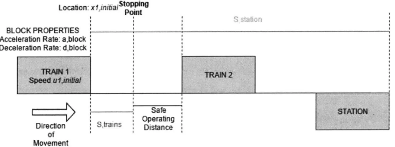
2.4.2.1: Start of Time-Step
At each time-step, every train in the system reports its speed uninitiol, location xninitial (where n is the train
ID, and x is taken relative to the first station in the line) and corresponding block acceleration and deceleration rates ablock and dblok to the Service Controller. The distance between the front of the train
and the end of the train in front of it, minus the safe operating distance, is calculated by the Controller and defined as strains. The distance between thefront of the train and thefront of the next station, sstation, is also calculated. This is shown for "Train 1" in Figure 2.8:
Location: xijnjifalStOPP'In
BLOCK PROPERTIES
Acceleraton Rate: ablock Deceleraton Rate: dblock
TRAIN TRAIN 2
Spee d u !.uilalTAI
-Sate
STATIONOperating Directon Strains Distance
of Movement
Figure 2.8: Defining Train Movement Variables
Now the remaining stopping distance s is calculated:
In Figure 2.9, the remaining stopping distance is strains, since Train 2 less the Safe Operating Distance is nearer to Train 1 than the station is.
The theoretical speed limit umax,t such that the train will have an adequate braking distance is obtained:
Umax,t = - 2dbLOCks (2.2)
If a safe operating headway tsafety is also implemented, a second theoretical speed limit umoxt2
corresponding to this condition is calculated as well:
Umax,t2 = stopping
tsafety
This is the speed at which the distance that the train would cover in the safe operating headway equals the distance to the train in front of it.
Umax,t and umax,t2 are then compared to the predefined system speed limit usystem and the actual speed
limit Umax actual is taken as the minimum of the three:
Umaxactual = min(umax,t, Umax,t2, Usystem) (2.4)
There are two cases that may result:
1) A "stopping case", where the train prepares to brake to a complete halt, and
2) A "speed adjustment case", where the train simply adjusts to a safer speed.
If the stopping point ahead is derived from the rear of the train ahead, and the speed of the train ahead is not zero, a "speed adjustment case" occurs. This is the case in Figure 2.8. Train 1 simply adjusts its initial speed ui,,nitiato the calculated limit Umaxactual by accelerating (if it is too slow) or decelerating (if it is too fast).