HAL Id: hal-02050982
https://hal-mines-albi.archives-ouvertes.fr/hal-02050982
Submitted on 27 Feb 2019
HAL is a multi-disciplinary open access
archive for the deposit and dissemination of
sci-entific research documents, whether they are
pub-lished or not. The documents may come from
teaching and research institutions in France or
abroad, or from public or private research centers.
L’archive ouverte pluridisciplinaire HAL, est
destinée au dépôt et à la diffusion de documents
scientifiques de niveau recherche, publiés ou non,
émanant des établissements d’enseignement et de
recherche français ou étrangers, des laboratoires
publics ou privés.
BEM computation of 3D Stokes flow including moving
front
M.-Q. Thai, Fabrice Schmidt, Gilles Dusserre, Arthur Cantarel, L. Silva
To cite this version:
M.-Q. Thai, Fabrice Schmidt, Gilles Dusserre, Arthur Cantarel, L. Silva. BEM computation of 3D
Stokes flow including moving front. International Journal of Material Forming, Springer Verlag, 2017,
10 (4), pp.567-580. �10.1007/s12289-016-1302-y�. �hal-02050982�
BEM computation of 3D Stokes flow including moving front
M.-Q. Thai1,5&F. Schmidt2&G. Dusserre2&A. Cantarel3&L. Silva4
Abstract Liquid composite molding (LCM) includes all composite-manufacturing methods, where the liquid state res-in is forced res-into the dry preformed reres-inforcement. In this study, numerical simulation of the resin infusion is presented based on a coupled approach involving Boundary Element Method (BEM) and Level Set Method. The method developed can handle stationary and transient flows by solving the Stokes equations. The numerical results on a square packed set of fibers show excellent agreement with the analytical model. The comparison between experimental and simulation results of flow front patterns revealed a fair accordance.
Keywords Liquid composite molding . Boundary element method . Level set . Resin flow
Introduction
Polymer matrix composites (PMC) reinforced by continuous fibers are characterized by their intrinsic heterogeneity and anisotropy. They require specific techniques of production [1] to obtain simultaneously the material and the geometry. This specificity allows designing a material suitable for the intended use. A unidirectional or multidirectional fibrous re-inforcement constitutes the skeleton of the composite material [2], constituted mainly of glass, carbon or other fiber types.
The preform usually comprises several layers organized into yarns, which are themselves composed of several thou-sands of fibers. The reinforcement geometry can be described at three different levels: the macroscopic scale (homogenized solid), the mesoscopic scale (layup or textile pattern) and the microscopic scale (local organization of a set of fibers [3]).
The use of liquid composite molding (LCM) is popular in many industrial applications. The main objective of LCM is to reach a full impregnation as the resin propagates between the fibers bundles and inside the bundles. The impregnation driv-ing forces result from pressure drop at macro-scale, but also from capillary forces at micro-scale. The competition between these driving forces in a dual-scale porous media results in non-uniform flow velocities that can cause impregnation de-fects such as micro-pores inside a tow, or macro-pores be-tween the tows [4].
To control the impregnation and avoid or at least limit these defects, the physical mechanisms involved must be accounted for. The physical parameters must be properly measured. The process parameters must be controlled (pressure, temperature, actual anisotropic permeability field related to reinforcement preforming depending on the shape of the part). A large work is thus compulsory to optimize this manufacturing process. * M.-Q. Thai
1 Faculty of Construction Engineering, University of Transport and
Communications, Hanoi, Vietnam
2 Mines Albi, ICA (Institut Clément Ader), Université de Toulouse,
Campus Jarlard, F-81013 Albi cedex 09, France
3 IUT de Tarbes; ICA (Institut Clément Ader), Université de Toulouse,
1 rue Lautréamont, F-65016 Tarbes, France
4 Ecole centrale de Nantes, ICI, 1 Rue de la Noë,
F-44300 Nantes, France
5 Research & Application Center for Technology in Civil Engineering,
University of Transport and Communications, Lang Thuong, Dong Da, Hanoi, Vietnam
To support the development of composites manufacturing, numerical simulation appears as an asset with regard to the shortening of the development time. In addition, it can anticipate the economic viability of the product, including manufacturing costs as well as the prediction of the actual composite properties. Driven by this need, numerical modeling addressing reinforce-ment preforming, mold filling and resin cure [5], has become an extensive field of investigation for the last three decades.
Modeling the resin flow through the reinforcement requires considering the relevant level depending on the aim of the model. Indeed, different modeling tools are involved at each level: flow in porous media (mainly Darcy’s law) at macro-scale [6], both flow in porous media (Darcy’s or Brinkman’s law) and Stokes flow at meso-scale [7] and mainly Stokes flow at micro-scale [8].
This paper focuses on the Stokes flow with two major issues. On the one hand, the identification of the permeability tensor of a porous media comprising several fibers organized randomly or following a regular pattern (useful to feed meso-scale models). On the other hand, the study of the transient resin flow front through the fibers that may lead to micro-pores formation.
With regard to the high complexity of the fibrous architec-tures, micro-scale flow modeling is usually carried out con-sidering a Representative Elementary Volume (REV), large enough to capture the average characteristics of the flow at a higher level. Typical applications can be found in literature regarding numerical permeability computation [7,8].
Boundary Element Method (BEM) utilized in this paper is an interesting alternative to Finite Element Method (FEM), for its mesh reduction to the domain boundary. Some authors report the use of this method in flow problems [9,10]. Its main diffi-culty is to calculate singular integral particularly in 3D cases. In addition, due to global assembling of the system matrix obtain-ed by the application of the BEM, problems of memory size are more tedious to handle. BEM only requires discretization of the surface rather than the volume. Another notable difference with FEM is that the degree of interpolation is the same for both unknowns (for example velocity and pressure).
This paper presented not only saturated flow cases but also focuses on the mold filling step of LCM process by coupling BEM and Level Set method. In this step, the resin is forced into the mold to impregnate the fibrous reinforcement. Moreover BEM is particularly well suited to be used in conjunction with the Level Set Method to address free surface problems, as the study of flow front propagation in a REV. Indeed, Level Set Method [11,12] is now considered as the most advanced nu-merical technique in the domain of mobile interfaces. It has been applied to various problems in quite different fields such as fluid mechanics, crystal growth in solid mechanics, edge detection in imaging. In recent years, there are many studies related to the moving interface in LCM processes using the Level Set method [13–15]. The coupling between BEM and Level set are also recently used for moving boundary problems [16,17] .
This work is based on an extension of prior work of Gantois et al. [18]. They investigate the use of boundary ele-ment method (BEM) to simulate the flows occurring at micro-scale in the reinforcement by solving Stokes equations with boundary integral formulations for two-dimensional flow. In our work, the numerical model of BEM is developed for the three-dimensional flow. Note that, the Green's functions, or fundamental solutions, are problematic to integrate as they are based on a solution of the system equations subject to a singularity load. Integrating such singular fields is not easy. For 2D case, analytical integration can be used. For 3D case, it is more difficult to design purely numerical schemes that adapt to the singularity. The new in this work is developed a numer-ical method to overcome that difficulty.
Our study deals with the development of a stationary and transient 3D BEM solver using Matlab® software framework capable of solving Stokes problem in saturated and unsaturat-ed environments. The results reportunsaturat-ed here aim to assess the validity of the solver by comparing numerical solutions to analytical and experimental data. The capillary forces are not accounted for in these results since this work is a first step toward a more complete modeling. First the application of BEM to solve Stokes problems is presented. Then the front tracking method is detailed, based on coupling of BEM and Level Set method [15,19], allowing to simulate free surface flows in unsaturated cases. The method is applied to estimate transverse and axial permeability, on a periodic arrangement of fibers. The numerical results are compared with analytical results of Gebart’s model [20] and Berdiche vsky et al. [21] and show that the BEM model in steady case for saturated flow provides relevant results of permeability in transverse and longitudinal direction. Finally, the unsteady free surface Stokes flow model is compared to experimental data obtained in such conditions that the capillary effects can be neglected. A fair agreement allows validating the numerical model.
Governing equations
In the following sections, we focus on the study of the flow at the microscopic scale, which is governed by Stokes equations. The Stokes flow is a particular case of the Navier–Stokes flow, where inertial forces are small compared with the viscosity contribution. These equations are relevant to model the low velocity-flow of a viscous fluid in small channels. The follow-ing assumptions are used:
1) Laminar flow, which corresponds to creeping flows where Reynolds numbers are low [22,23].
2) Incompressible Newtonian fluid.
3) Motionless condition for the fibers. In this paper, the in-fluence of reinforcement deformation [24] is not accounted for.
4) Gravity force is neglected.
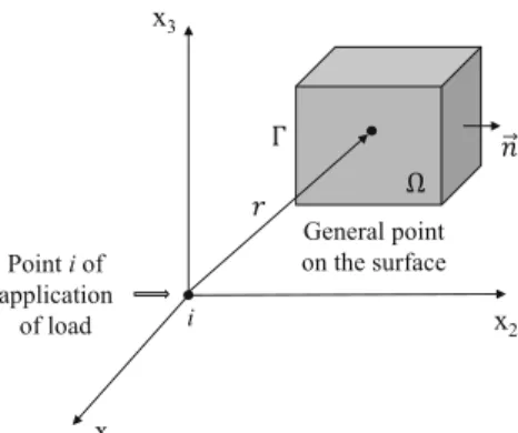
In the following,Ω is an isotropic medium filled by a ho-mogeneous fluid phase in equilibrium on which the stokes equations applies (Fig. 1),Γ is the set of boundaries of the domain. The outward normal to the boundary is defined as n. r is the Euclidean distance between the current point and the collocation point. If the aforementioned assumptions are ver-ified, the well-known Stokes equations govern the motion of the fluid through the domain, Eq. (1).
μΔv ¼ ∇p ∇v ¼ 0 !
in Ω ð1Þ
Where v is the fluid velocity and p the pressure. Two types of boundary conditions can be applied:
i. vi¼ vionΓvi (imposed velocity)
ii. ti¼ tionΓti (imposed stress vector)
where viand tiare the prescribed i-component of velocity
and stress vector on the boundary.
The normal stress vector at the boundary is given by ti= σijnj, with njbeing the component j of outward normal at
boundary.
The stress tensor σ is described using a Newtonian behav-ior law for the resin:
σ ¼ −pI þ 2μD D ¼12 ∇vþt∇v
ð Þ
(
ð2Þ where D is the strain rate tensor, I the second-order identity tensor, μ the dynamic viscosity of the fluid.
Numerical method
This section details the BEM used to solve the fluid flow around bodies with arbitrary geometries [9,10]. In this meth-od, only a boundary mesh is used instead of a full domain
mesh. In fact, we developed here a BEM method used the given boundary conditions to fit boundary values into the integral equation, rather than values throughout the space de-fined by a partial differential equation. Once this is done, in the post-processing stage, the integral equation can then be used again to calculate numerically the solution directly at any desired point in the interior of the solution domain [9]. The method is composed of the following steps: discretization of the integral equation, evaluation of the integrals, application of the boundary conditions, generation of the final system of equations, and finally, calculation of the velocity and stress. A fundamental solution (so called Green function) is required in order to eliminate the domain integral. This fundamental so-lution changes with the nature of the problem [9].
The treatment of a moving flow front has been imple-mented at micro-scale, and is based on coupling a Level Set method together with the Marching Tetrahedra meshing procedure [25]. Note that, in unsaturated case, we need to re-mesh for simulating the flow even for the FEM method [26,27].
There are in the literature different types of elements [10] defined by the degree of interpolation and continuity (constant elements, linear continuous, discontinuous linear, quadratic, etc.…). Constant elements are developed in this paper. So, both fields, velocity and pressure, will be considered to be constant on an element and equal to the value at the center of the element. The centers of the elements (i.e. the collocation points) are going to be used as the points where the integral equations are applied. The boundary elements used in this work are three-node triangles for 3D domains.
In BEM, fundamental solutions are the key points. There are different fundamental solutions for two-dimensional and three-two-dimensional problems. In this pa-per, only a fundamental solution for isotropic materials is presented (even fundamental solutions exits for the case of three dimensional anisotropic with spatially case [9,28, 29], but they are very difficult to use because of the com-plexity of their mathematical formulation or the need to find part of the solution numerically). The boundary inte-gral formulation for Stokes’ flow is derived from elastostatic formulation (refer to [30] for further details).
In the boundary element method, we perform a second integration by parts to transform the integral area in equa-tion. The application of the divergence theorem allows achieving the integral equation. The 3D BEM for Stokes is very similar to the 2D, ruled by the set known as Somigliana’s equations: Z Ω ∂σ* k j ∂xj vkdΩ ¼ Z Γ t* kvkdΓ− Z Γ tkv*kdΓ ð3Þ
Where vk*is the virtual velocity and tk*is the virtual stress.
Ω is the computational domain (resin), Γ is the boundary.
x2 x1 x3 Point i of application of load General point on the surface Ω Γ i
It is noteworthy that both boundary integral equations and fundamental solutions remain valid, and involve now ve-locity and stress vectors. A fundamental solution σkj* is
required in order to eliminate the domain integral of the problem: v* lkðx; sÞ ¼ 1 8πμrðδlkþ rlrkÞ t* lkðx; sÞ ¼ − 3 4πr4!: nr ! 8 > < > : ð4Þ
r is the Euclidean distance between the current point and the collocation point (Fig. 1), n! is the outward normal. δlk is the Kronecker symbol.
In order to solve the discretized set of Eq. (3), we follow the standard procedure to construct the global set of equations. Boundary conditions are introduced, assigning the prescribed nodal values. Passing all unknowns on the left-hand side by permuting columns, we obtain a linear system ready to be solved.
As previously, it is considered here that the surface Γ of domain Ω is discretized into N boundary elements and putting the point s at node i of coordinates xiyields to the discrete form of Somigliana’s equation (Eq (3)) [9, 31] given as: δlkvk" #xi þ XN j¼1 Z Γj t* lk x; xi " # dΓjð Þx 2 6 4 3 7 5vk" #xj ¼X N j¼1 Z Γj v* lk x; xi " # dΓjð Þx 2 6 4 3 7 5tk" #xj ð5Þ
vlk* and tlk* represent the velocity and stress in the k
direc-tion due to a unit load in the l direcdirec-tion acting at i.which can be summarized using block partitioned matrices as follows
H
½ & v½ & ¼ G½ & t½& ð6Þ
where [v] (respectively [t]) is a 3x1 matrices storing the velocity vector (respectively, the stress vector) at the node and [H], [G] are 3x3 full submatrices calculated by :
Hijlk ¼ 1 2δi jδlkþ Z Γj t*lk"x; xi#dΓjð Þx Gijlk ¼ Z Γj v* lk x; xi " # dΓjð Þx 8 > > > > > < > > > > > : ð7Þ
The only real difference between the 3D and 2D cases is how to numerically evaluate the term in each integrand of
Eq. (7). The integral expressions of submatrices G and H (Eq. (7)) are evaluated using a numerical method. Particularly for the case with the singularity where the collo-cation point belongs to the element, i.e. i = j, the expression of H is given as follows
Hiilk¼1
2δlk ð8Þ
However, the integrals of Eq. (7) for the G matrix in 3D will not be available via an analytical formula like in the 2D case. Therefore, these integrals have to be computed using a large number of point Gauss quadrature formulas or another numerical method, like Telles, described in the following subsection.
Numerical integrations
One of the differences between BEM and FEM method is that the integrals in BEM are more difficult to evaluate than in FEM and can sometimes contain integrals of sin-gular functions. Due to the particular shape of the funda-mental solution, the classical Gauss scheme for numerical integration proves to be much more difficult, especially, when the distance r (Fig. 1) between the collocations point i and integration point j is low. A singularity arises when i belongs to the element, causing a problem during the assembly of the terms of the block diagonal matrix G. In the case of the matrix H, this problem can be overcome by considerations of rigid body motion, and calculated directly (see previous Eq. (8)).
The accurate numerical integration of integrals is very im-portant for a reliable implementation in BEM. Usually, the regular integrals arising from an implementation are evaluated using standard Gaussian quadrature. However, the singular integrals that arise are often evaluated through another way, sometimes using a different integration method with different nodes and weights. This paper presents a simple transforma-tion to improve the accuracy of evaluating weakly singular integrals.
Indeed, one can notice that the fundamental solution for three dimensions is the function with singularity at 1/r and 1/r2: u* lk ¼ Θ 1 r $ % and t* lk¼ Θ 1 r2 $ % ð9Þ It is well known that conventional Gaussian quadrature becomes inefficient or even inaccurate when applied to evaluate these integrals directly. Then, to improve the re-sults, we can use a large number of Gaussian points [32], clearly an inconvenient, since calculation times become much longer. The integral always appears in the assembly
step (diagonal) of G matrix. Hence, it is particularly im-portant to implement an appropriate strategy of computa-tion. The solution depends strongly on the level of accu-racy made to evaluate these terms. There are in the liter-ature different types of approaches to solve this problem: analytical integration [33], the integration subdivision el-ement, or the technical processing area. Following this idea, the contribution of Telles [34] is one of the most popular. The aim of this technique is to consolidate the integration points around the singularities in order to weaken or cancel out these singularities by using the Jacobian of the transformation. Then, it applies the ordi-nary Gauss rule for integral calculation. Both methods are compared in this section: using a large number of Gauss points and the contribution of Telles, to compare their efficiency.
The comparison between both methods is performed based on the integration given in Eq. (10), which presents a singu-larity at ε =0 or η =0. f ε; ηð Þ ¼ Z1 0 Z1 0 log 1 ε $ % log 1 η $ % dεdη ð10Þ
The two-dimensional Gauss quadrature formula provides Eq. (11), whereas Telles formula is obtained by using the Jacobian of the transformation before applying the ordinary Gauss rule, Eq. (12).
I ¼ Z1 0 Z1 0 f ε; ηð Þdεdη≅X n j¼1 Xn i¼1 f εi; ηj & ' wi; wj ð11Þ I ¼ Z1 0 Z1 0 f ε; ηð Þdεdη ¼ Z1 0 Z1 0
f ε η& & '; η η& ''dεdη≅X n j¼1 Xn i¼1 f εi η & ' ; ηj η & ' & ' wi; wjJTi JTj ð12Þ
Where η is the coordinate of the singular point, JTis
Jacobian of transformation.
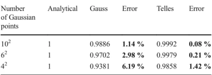
Table 1 presents the comparison between both methods of integral evaluation of Eq (10) and its analytical solution. This comparison shows that Telles method provides better results than Gauss method even with a reduced number of integration points. In the following, Telles formula will be used to evaluate the singular integrals in the stationary saturated case. However, in the transient case with free surface, to easily couple Level Set and Marching Tetrahedral, Gauss Quadratic method is used with a large number of Gaussian points despite the consuming time calculation.
Level set and marching tetrahedra
The moving flow front is computed using a Level Set approach. The formulation allows taking into account flows with complex
topologies, including merging of several flow fronts. By using the signed distance function, the method allows a continuous capture of moving boundaries, which allows calculating precise-ly the shape of the flow front. Level set theory indicates that the front motion is governed by the boundary velocity field. As a result the use of BEM together with level set techniques is straightforward to compute the filling pattern. At first, the bound-ary or flow front,Γ can move and filling with fluid over time. The benefit of combining BEM and Level Set is the reduction of the domain calculation to the boundary calculation, which mo-tion is fully determined by its normal velocity.
Let us consider an interfaceΓ(t), with a shape that changes with time and is defined in Rn. It is assumed that the interface
motion is limited in a domainΩp, defined by the whole cavity.
The interface, defined by the Level Set value of zero, depends on space and time according to Eq. (13), where M is a fixed point, n is the problem dimension (n = 3 in this case), and∅ is the Level Set function.
Γ tð Þ ¼ M∈Rf n; ∅ M; tð Þ ¼ 0g ð13Þ
Conventionally, the different subdomains are identified thanks to Eq. (14), where ∅ (M, t) = d(M, Γ(t)) is the Euclidean distance from the point M to the boundaryΓ.
∅ M; tð Þ < 0 if M∈ Ω tð Þ ∅ M; tð Þ ¼ 0 if M∈ Γ tð Þ ∅ M; tð Þ > 0 if M∉ Ω tð Þ 8 < : ð14Þ
Table 1 Comparison between Telles method and Gauss quadrature
formula Number of Gaussian points
Analytical Gauss Error Telles Error
102 1 0.9886 1.14 % 0.9992 0.08 %
62 1 0.9702 2.98 % 0.9979 0.21 %
The coupling of BEM and Level Set is performed using Eq. (15), where vnis the Euclidian norm of the extended normal
velocity. The initial value of the Level Set function,∅0, is
eval-uated through a direct calculation from the background nodes. ∂∅
∂t þvnj∇∅j ¼ 0 ∅ M; tð 0Þ ¼ ∅0 (
ð15Þ At each time step, the Level Set function is determined using a first order discretization, Eq. (16), where the time step Δt is calculated using the Courant-Friedrichs-Levy formula, Eq. (17).
∅ M; t þ Δtð Þ ¼ ∅ M; tð Þ−vnðM; tÞ ∇∅ M; tj ð ÞjΔt ð16Þ Δt ¼ cv δ
n;max ð17Þ
That condition is necessary for convergence while solving the partial differential equations. We use the stability condition Courant-Friedrichs-Lewy, who restricts movement of the boundary at the background grid on a time increment
If the Level Set field is known, then we can compute the position and shape of the moving boundary through its zero iso-value. After calculation of the Level Set function, the boundary mesh is updated at each time step using the background grid through a Marching Tetrahedra algorithm [25]. The method of Marching Tetrahedra is a direct ex-tension of Marching Triangles [35]. In this algorithm, each tetrahedron is investigated to determine how the front intersects the grid. Sixteen intersection cases can be encountered, but they reduce to only four topologies using symmetry and nodal permutations. It is noteworthy that this method generally generates a large number of elements in the boundary mesh. However, it is easy to reduce significantly unnecessary elements using a pertur-bation procedure acting on the Level Set data [36].
The filling of the domain is divided into a finite number of quasi-static states. After the BEM calculation, pressure and nor-mal velocity are determined at the boundaries. Then, the nornor-mal velocity is used to update Level Set field using Eq (16) to update the boundary mesh. In order to ensure the condition of non-penetration, at each time step, the current Level set value is modified by intersecting mold with resin front using Eq. (18):
∅ ¼ max ∅; ∅ð mÞ ð18Þ
where∅mis the signed-distance function to the mold walls.
Comparison with analytical and experimental results
The purpose of this section is to assess the ability of the im-plemented methods to simulate three-dimensional flows decoupled from cure kinetics, thermal analysis andreinforcement deformations. Firstly, the micro scale steady model is tested by computing the transverse and longitudinal permeability of an idealized periodic pattern of fibers orga-nized into square packing. Finally, some experimental results are compared with numerical solutions of an unsteady free surface flow where capillary forces can be neglected. Comparison of 3D steady flow simulation with analytical results
The main characteristic of a preform, necessary to simulate resin flow at macro- or meso-scales is its permeability tensor. In most cases, its value can be determined using experimental devices [37]. However, permeability depends strongly on mi-crostructure and to a lesser extent on other parameters such as vacuum pressure, and the random distribution of fibers leads to an important dispersion of the results together with exper-imental difficulties ([38,39]). Therefore, many works have been devoted to the development of analytical formulae to compute permeability in particular geometries [20,40]. In this section, the BEM simulations are compared with analytical reference solutions of permeability values.
This approach enlarges the results of a preliminary work [30], that compared the transverse permeability computed using 2D-BEM with the well-known Gebart analytical solu-tion [20]. In the present work, 3D BEM computasolu-tions in a square arrangement of straight fibers provide both transverse and longitudinal permeability that will be compared to analyt-ical results. The first analytanalyt-ical solution is provided by Gebart formula [20] that express the transverse and longitudinal per-meability in a square fibers packing as a function of fiber volume fraction. In this model, the analytical treatment of creeping flow perpendicular to the axis of the fibers is predi-cated. The assumptions used are that permeability is con-trolled by the narrow gaps formed between the fibers, and that the width of these gaps varies only slowly.
In Gebart’s model, Stokes equations are analytically solved, assuming thin flow channel, rigid, fixed and impermeable fibers together with a sticking contact. The transverse permeability Kt
is given by Eq. (19), where R denotes the fiber radius and Vfthe
fiber volume fraction. π/4 value corresponds to the maximal fiber volume fraction with contacting square packed fibers. Kt¼ 16 9πpffiffiffi2 ffiffiffiffiffiffiffiffiffiπ 4Vf r −1 $ %5=2 R2 ð19Þ
According to similar assumptions, Gebart also proposes the longitudinal permeability expression, Eq. (20), where Klis the
axial permeability. Kl¼ 8 57 1−Vf " #3 V2 f R2 ð20Þ
Equation (20) usually provides less acceptable results than Eq. (19) because the actual longitudinal flow fails to match the assumptions made. The solution proposed by Berdichevsky [21], Eq. (21), resulting from analytical developments fitted on finite element computations, will be considered as refer-ence solution for the longitudinal case.
Kt¼ A 1− ffiffiffiffiffiVf Vu q & '5=2 ffiffiffiffiffiV f Vu q & 'n R2 Kl¼exp B þ C:Vf " # Vm f R2 8 > > > > > > < > > > > > > : ð21Þ Where A = 0.244 + 2(0.907− Vu)1.229; B = 5.43− 18.5π/4 + 10.7(Vu)2; C =− 4.27 + 6.16Vu− 7.1(Vu)2; m =− 1.74 + 7.46Vu− 3.72(Vu)2; n = 2.051 + 0.381(Vu)4.472.
Similarly as Gebart equation, this model assumes that the permeability of a fiber assembly is influenced by the fiber volume fraction Vf. It also is influenced by the packing pattern
characterized by the ultimate volume fraction Vu, equal to π/4
in the square packing case.
Another study of Bruschke and Advani [41] found that one could use lubrication theory and the cell model concept to describe permeability across an array of fibers as a function of fiber volume fraction
K ¼r 2"1−L2# 3L3 3Ltan−1 ffiffiffiffiffiffiffi1þL 1−L q ffiffiffiffiffiffiffiffiffiffi 1−L2 p þL 2 2 þ1 0 @ 1 A −1 ð22Þ Where L2= 4Vf/π and r is fiber radius. Note that no
empir-ical parameters were needed.
In order to make comparisons with the aforementioned analytical models, a BEM solution was computed for the same square-packing configuration for a flow either perpendicular or parallel to the fiber axis. The geometry and the prescribed boundary conditions are sketched in Fig.2: a no-slip condition at the surface of the fiber for both longitudinal flow (Fig.2b) and transverse flow (Fig. 2a). Sliding conditions were im-posed to account for the symmetry planes. A pressure drop was imposed by setting a uniform pressure at both inlet and outlet.
The permeability value is computed from the flow exiting the REV (Representative Elementary Volume) by integrating the normal velocity field and using Darcy’s law, Eq. (22): K ¼μ 1−Vf " # pin−pout Z Γout v:n dΓ ð23Þ
whereΓoutis the REVoutlet boundary, μ is the dynamic viscosity
of the fluid, v is the velocity of the fluid, pinand poutare pressure at
inlet and outlet respectively. Vfis the fiber volume fraction.
The permeability value is also calculated by Finite Element Method. By calculating the average velocity from FEM sim-ulation in Comsol 4.2 Software, knowing the pressing drop Δp = pin− pout over the length of the unit cell, and using
Eq. (23) the permeability values are obtained.
All models were compared from data computed with fiber volume fraction ranging between 0.1 and 0.7. The radius of the fiber was set to 10μm, corresponding to an average value for a glass fiber. The increase in the volume fraction is obtained by decreasing the inter-fiber space. A boundary mesh is only required with BEM method. The surface normal velocity is computed first and then the permeability value is calculated using Eq. (23).
Equation (23), which involves only a boundary field veloc-ity, shows that the calculation can be carried out using a fully surface approach. BEM allows accessing directly to the bound-ary velocity without calculating any volume variable inside the 3D domain. It is clear that this approach is an alternative to the powerful finite element method that requires more advanced meshing tools. Thus, one of the seven cases of calculation was complete in less than 10 min on a PC with a CPU 2.26GHz/8GB Ram with about 3000 boundary elements.
A plot of the transverse permeability versus fiber volume fraction is presented in Fig.3. The comparison of the analyt-ical results and numeranalyt-ical simulations shows that all models provide very similar permeability values, and perfectly agree for fiber volume fraction higher than 0.4. Below this value, BEM solution is between Gebart, Bruschke and Berdichevsky results and FEM simulation (Comsol 4.2 software) but the discrepancy remains very low.
The value of longitudinal permeability obtained using BEM and analytical formulae are in the same order of magni-tude. However, the results reported in Fig.4 show that all Fig. 2 Boundary conditions for
transverse (a) and longitudinal flow (b)
models do not provide the same trend. Indeed Gebart’s model overestimates the permeability value for low fiber volume fraction and underestimates it for high fiber volume fraction. However both Berdichevsky formula and BEM simulations and also FEM simulation properly match together over the entire range of fiber volume fraction. These results confirm that the 3D BEM model provides relevant results for 3D steady flow under Stokes conditions.
Comparison of 3D unsteady free surface flow simulation with experimental results
Experimental setup
This section is devoted to the validation of a 3D free surface flow simulation in the unsteady case by comparison to
experiments. The flow experiment was conducted in a cavity whose dimensions (477mmx117mmx2mm) are sufficiently large to neglect the capillary forces, at low velocity to match the Stokes flow conditions. The objective of this test is to capture experimental flow front patterns at several times to compare with the numerical results. In order to provide flow front patterns similar to those encountered in the intended application, i.e. the flow of resin around a set of fibers, some 26 mm-diameter circular rubber obstacles were located sym-metrically in the cavity (Fig.5), leading to front merging and separation. In this experiment, canola oil was used as a model fluid for its appropriate properties (perfect incompressibility and Newtonian behavior [22]). The test was performed at room temperature in order to match isothermal conditions. The obstacles are motionless during the test and considered as rigid. Note that the process is monitored optically. The
0 0.1 0.2 0.3 0.4 0.5 0.6 0.7 0.8 10−4 10−3 10−2 10−1 100 101 Vf K/R 2 BEM Gebart FEM Berdichevsky Bruschke and Advani
Fig. 3 Transverse permeability: comparison between BEM and other models 0 0.1 0.2 0.3 0.4 0.5 0.6 0.7 0.8 10−4 10−3 10−2 10−1 100 101 Vf K/R 2 BEM Gebart FEM Berdichevsky Fig. 4 Longitudinal permeability: comparison between BEM and other models
images are captured at a rate of 4 frames per second thanks to a CDD camera placed above the setup. The inlet and outlet pressures were measured with strain gauges based miniature pressure transducers. The experimental data including the dy-namic viscosity and specific mass of the fluid are given in Table2.
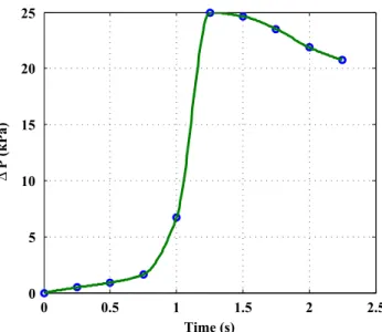
The pressure drop between inlet and outlet is not constant with time (Fig.6). A nominal relative air pressure of 25 kPa was applied on the fluid tank inside a chamber thanks to a pressure reducer. At the beginning of the test, the inlet pres-sure increased exponentially from atmospheric prespres-sure. When the pressure drop reached 25 kPa at inlet, the pressure reducer went off and the inlet pressure decreased slowly to tend toward a pressure drop of 20 kPa. Figure 6 shows the pressure drop measured during the experiment. These actual values of pressure drop were taken into account in the simu-lation as boundary conditions.
The assumptions of the BEM model include creeping flow hypothesis (Stokes flow). Low Reynolds number Re will in-dicate if the inertial effect can be neglected compared to vis-cous contribution. It is defined by Eq. (23), where v is average velocity of the fluid and D is the hydraulic diameter.
Re ¼ρvDμ ð24Þ
The experimental results indicate that the time for complete filling is about t = 2.25 s, so the average velocity of the flow is about v = 0.1 m.s−1. The hydraulic diameter is defined by D = 4A/P (A is the cross-sectional area and P is the wetted perimeter). Considering a rectangular cross-section with a mold thickness e very small compared to the width L, e≪ L, then D = 2e and finally computing Reynolds number gives Re ≃ 4.9. This value of Reynolds number is very low compared to the critical value 1400 which is the minimum critical
Reynolds number for laminar-turbulent transition [42]. It can thus be considered that the assumption of laminar flow is acceptable in this experiment, as well as the assumptions of quasi-steady flow, fluid incompressibility and Newtonian behavior.
In our work, we assume that the effect of gravity is neglected based on the study of the Froude number [43], which represents the relative importance of inertia forces to gravity forces, Eq. (25). Where g is acceleration due to gravity, Lcis characteristic length (in our case Lc= e).
Fr ¼ v 2
gLc ð25Þ
Equation (25) allows computing a numerical value of Froude number of approximately 0.5. This value shows that both effects of inertia forces and gravity forces have the same order of magnitude. This is the reason why the gravity force is neglected.
Similarly, the relative effect of viscous forces versus sur-face tension is represented by the modified capillary number, Eq. (26), where the surface tension of canola oil is γ = 32.10− 3Nm− 1[44], the viscosity of canola oil is given in Table2, and θ is the contact angle between the fluid (canola oil) and solid (steel). This angle depends on the surface rough-ness and its value is around 83° [45]:
Ca ¼γcos θvμ
ð Þ ð26Þ
We can finally find out the value of the modified capillary number, Ca≈ 2. This means that the capillary effect again is less important than viscous effect.
The assumptions considered to develop the present model of resin flow at microscopic scale are verified, as proved by Fig. 5 Experimental setup
Table 2 Experimental parameters
μ (Pa.s) ρ (kg.m−3) rinlet(m) robstacle(m)
0.075 916 9e-3 13e-3 0 0.5 1 1.5 2 2.5 0 5 10 15 20 25 Time (s) ∆ P (kPa)
Fig. 6 Pressure drop change measured during the test. The dots correspond to times were images were captured
the calculation of Reynolds and Froude numbers. These di-mensionless numbers are very important because their calcu-lation already provides very important information about the flow before solving the Stokes equations.
These dimensionless numbers at both scales can be com-pared in order to verify the validity of these hypotheses. Let us first consider the Reynolds number (Eq.23).
Because the resin density ρ, and the viscosity μ are as-sumed constant, only the study of the variation of the velocity v and the hydraulic diameter D is needed.
At the test-scale, the velocity of the resin has the order of magnitude 0.1 m/s and the hydraulic diameter: 4 mm, while at the microscale, the velocity of the resin has the order of mag-nitude 10−1- 10−2m/s (see [30,46]), and the hydraulic diam-eter : 10−6m.
So from Eq. (23), we see that the Reynold number at mi-croscale is still smaller than that at test-scale. Then, inertia terms can be neglected. So, the assumption of laminar flow is always valid at microscale.
Similarly, the ratio of the order of magnitude between the Froude number at test-scale FrIand at microscale FrIIis
ob-tained through equation below: FrI FrII ¼ v2 I v2 II LcII LcI ¼ 10 −3−10−5 ð27Þ
It turns out that the Froude number at test-scale is smaller than that at microscale. This means that the gravity effect is less important than the inertia effect. Therefore, the gravita-tional force may be neglected.
In conclusion of this section, from dimensional analysis, we find that the assumptions used in this study are also valid for the flow at the microscale, except the effect of capillarity since the experiment was design in such a way that this phe-nomenon can be neglected.
Simulation of the experiment
Numerical computations were performed to simulate the free surface flow in the first half of the cavity where the obstacles were located. Two kinds of mesh are needed to simulate the flow. The first one is a background grid. It is generated by a
standard tetrahedral element mesh. The other mesh is a com-putational boundary mesh, which bounds the fluid phase at each step time. The 3D grid mesh (Fig.7) is established with 4589 nodes and 17264 tetrahedral elements, including 6352 boundary triangle elements and 3162 boundary nodes. The mesh was parameterized with 4 elements through the thick-ness (see Zoom (fig.7.a in Fig.7).
The Reynolds number calculation allows assuming that the flow can be modeled using Stokes equations. Moreover, the flow is described as a succession of quasi steady states. At each time step, governing equations are solved using BEM. The flow front is then updated by coupling BEM with Level Set method. A Marching Tetrahedra algorithm is applied to generate a boundary mesh at each time step. The process is repeated until the mold is completely filled. The following boundary conditions were prescribed to simulate the flow ex-periment. The actual pressure drop (Fig.6) was imposed uni-formly on a cylindrical surface in front of the mold inlet as-suming that the cavity is thin enough to neglect the pressure drop through the mold thickness. No-slip conditions were im-posed at all solid boundaries, where the fluid is in contact either with the mold or with the rubber obstacles.
The simulation was carried out using a PC (2.26GHz, 8GB of RAM) with a CPU time of 12 h to perform the complete filling of the mold.
In the present work, a simple version of BEM was devel-oped which still needs to be optimized and the comparison with the computation time of commercial FEM in this case would not make sense.
On other aspect, BEM is also well suited to combine with Level Set Methods, as they use the signed-distance to the interface to follow the front motion. By using the signed-distance function, the method allows a continuous capture of the moving boundary, which allows calculating accurately the form of the flow front. Hence, in several cases, coupling BEM and Level Set methods can achieve significantly better preci-sion than FEM.
Discussion
The numerical flow front patterns are compared in this sub-section to those captured at several times during the Fig. 7 Background 3D grid
mesh: injection inlet (a) and reinforcements (b)
experiment. Each image (Fig.8a) was analyzed with commer-cial Aphelion software to extract the boundary pixels (Fig.8b). The numerical simulation and the experimental flow front pattern were then superimposed (Fig. 8c) to achieve comparisons.
The experimental and numerical flow fronts are com-pared at different time steps on Fig. 9. In most of the cases, a good agreement can be observed between both simulated and experimental flow front patterns. At the
beginning, the fluid enters quickly into the mold (Fig. 9a and b) and then flows through the obstacles (Fig. 9c–e). Even when the flow front meets obstacles, the simulation provides flow front patterns very similar to those measured thanks to image analysis. This shows the ability of BEM model to describe properly the flow front patterns occurring at lower scales during the filling of yarns.
It is important to notice that the main feature of the BEM is the use of a boundary mesh instead of a full domain mesh. With boundary elements, there is no need to refine the domain elements, but simply discretize only the boundary mesh. In our work, the boundary mesh is updated at each time step using the background grid through a Marching Tetrahedra algorithm. Note that the boundary mesh for the next increment is built by the in-tersection of the volume mesh and the position of the Level Set function computed at the current increment. It means that the flow front is immersed in the fixed volume mesh. This background grid is only used to define the free surface mesh. The results in Figs. 7,8 and 9 present the advancing front of the resin at each time step and to be meshed by only boundary mesh, not full domain mesh. Therefore, this method is less time consuming in term of mesh generation. In order to calculate the variables (pres-sure, velocity…) at any desired node of the 3D domain, there is no need to solve again the equations; but just to post-process the surface solution previously computed.
Figure10 details the flow front pattern computed be-tween two obstacles by highlighting the tridimensional description of the flow. The computed flow front is quite disturbed due to a coarse mesh and related to the thin cavity. Indeed, a parabolic velocity profile may arise in the thickness of the flow and would require a finer mesh to accurately reproduce the flow front shape. However, this does not globally influences the macroscopic flow front pattern response.
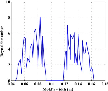
To further investigate the validity of the assumptions in this experiment, the local values of the Reynolds number have been computed thanks to simulated results. Figure11presents the Reynolds number value at the mov-ing fluid boundary at the last iteration of simulation, t = 1.75 s (Fig. 9e). These values are assessed using Eq. (24). In this case, v is the velocity at the center of each element and D is the hydraulic diameter. Note that
(a)
Original image(b)
Extraction of boundarypixels
(c)
Superposition resultsFig. 8 Image processing (Aphelion and Matlab)
(a)
Time : 0.25s(b)
Time : 0. 5s(c)
Time : 1.25s(d)
Time : 1.5s(e)
Time : 1.75sFig. 9 Comparison between experimental and numerical flow front patterns
the hydraulic diameter is based on the actual cross section area. The boundary elements used are three-node trian-gles. Therefore, the hydraulic is approximately equal the diameter of the circumscribed circle of each triangular element.
This diameter depends thus on the element size, ranging in the present study between 1.5 mm and 5.5 mm. The Reynolds number ranges between 0 (at contact with mold and fibers due to the sticking contact) and 8. The average value is close to the global Reynolds number assessed above. These values are very low compared to the critical value of the transition laminar-turbulence (about 1400 [47]), showing that the local effects are small enough and that Stokes flow assumption is still relevant.
Conclusion and prospects
This paper develops a numerical model to simulate the flow occurring at the fiber-scale in LCM processes by using the BEM method. The advantage of this model is that only the surface of domain is meshed, allowing an easier meshing step. The numerical model developed in this work is dedicated to solve quasi-static 3D Stokes problems and to account for free surfaces (flow fronts).
The scope of this paper is the validation of numerical simulations by comparison to analytical and experimental data. The case mentioned is devoted to the identification of the transverse and longitudinal permeability. The cal-culations without moving free surface have been per-formed on a square packing of fibers and reveal an excel-lent agreement with the relevant analytical models.
The relevance of the quasi-static free surface solver to sim-ulate Stokes flow was analyzed by comparison to the results of a macro-scale fluid flow experiment. This test involves some circular obstacles to reproduce the flow front merging and separation occurring at the micro-scale during the impregna-tion of a tow. The size of the cavity allowed neglecting the capillary effects. This comparison shows that the numerical simulation is able to provide a fair description of the flow front pattern.
Further improvements of the model can be performed to account for the deformation of the fibrous reinforce-ment, and more realistic boundary conditions between the fluid and the fiber surface (wettability, capillary ef-fects, surface tension). It would provide the possibility to study the origin and the development of voids during the process, which is an important indicator of the quality of processing composites parts.
Acknowledgments This work was carried out in the framework of the collaborative French project BDe l’image au maillage^ coordinated by Mines Telecom Institute (IMT). The authors gratefully acknowledge S. Leroux for her contribution to this work. Author Minh-Quan THAI has received research grants from the Vietnam National Foundation for Science and Technology Development (NAFOSTED) under grant num-ber 107.02-2015.17. The other authors declare that they have no conflict of interest.
References
1. Beukers A (2001) Polymer matrix composites : applications. Encyclopedia of Materials : Science and Technology. Elsevier, Oxford. p 7384–7388
2. Jones RM (1998) Mechanics of composite materials. CRC Press 3. Gantois R (2012) Contribution à la modélisation de l’écoulement de
résine dans les procédés de moulage des composites par voie liquide. In Thesis. Université de Toulouse
4. Patel N, Lee LJ (1995) Effects of fiber mat architecture on void formation and removal in liquid composite molding. Polym Compos 16(5):386–399
Fig. 10 Zoomed area of the front flow at t = 1.5 s 0.040 0.06 0.08 0.1 0.12 0.14 0.16 0.18 2 4 6 8 10 Mold’s width (m) Reynolds number
5. Rouison D, Sain M, Couturier M (2004) Resin transfer molding of natural fiber reinforced composites: cure simulation. Compos Sci Technol 64(5):629–644
6. Gantois R, Cantarel A, Dusserre G, Félices JN, Schmidt F (2010) Numerical simulation of resin transfer molding using BEM and level set method. Int J Mater Form 3(1):635–638
7. Silva L, Puaux G, Vincent M, Laure P. A monolithic finite element approach to compute permeabilityatc microscopic scales in LCM processes. Int J Mater Form 3(1):619–622
8. Chen X, Papathanasiou TD (2007) Micro-scale modeling of axial flow through unidirectional disordered fiber arrays. Compos Sci Technol 67:1286–1293
9. Brebbia CA, Dominguez J (1992) Boundary elements: an introduc-tory course. Computational Mechanics Publications, 2nd edition 10. Paris F, Canas J (1997) Boundary element method : fundamentals
and applications. Oxford University Press
11. Osher S, Sethian JA (1988) Fronts propagating with curvature-dependent speed: algorithms based on Hamilton-Jacobi formula-tions. J Comput Phys 79(1):12–49
12. Sethian JA (1999) Level set methods and fast marching methods evolving interfaces in computational geometry, fluid mechanics, computer vision, and materials science. Cambridge University Press, 2e édition
13. Liu Y, Moulin N, Bruchon J, Liotier P-J, Drapier S (2016) Towards void formation and permeability predictions in LCM processes: a computational bifluid–solid mechanics framework dealing with capillarity and wetting issues. Comptes Rendus Mécanique 344(4–5):236–250
14. Abouorm L, Moulin N, Bruchon J, Drapier S (2013) Monolithic approach of Stokes-Darcy coupling for LCM process modelling. Current state-of-the-art on material forming: numerical and experi-mental approaches at different length-scales, PTS 1–3. 554–557: 447–455
15. Trochu F, Ruiz E, Achim V, Soukane S (2006) Advanced numerical simulation of liquid composite molding for process analysis and optimization. Compos A: Appl Sci Manuf 37(6):890–902 16. Colicchio G, Greco M, Faltinsen OM (2006) A BEM-level set
domadecomposition strategy for non-linear and fragmented in-terfacial flows. Vol. 67. Chichester, ROYAUME-UNI: Wiley. 1385–1419
17. Garzon M, Adalsteinsson D, Gray L, Sethian JA (2005) A coupled level set-boundary integral method for moving boundary simula-tions. Interfaces Free Boundaries 7(3):277–302
18. Gantois R, Cantarel A, Cosson B, Dusserre G, Felices J-N, Schmidt F (2013) BEM-based models to simulate the resin flow at macro-scale and micromacro-scale in LCM processes. Polym Compos 34(8): 1235–1244
19. Soukane S, Trochu F (2006) Application of the level set method to the simulation of resin transfer molding. Compos Sci Technol 66(7– 8):1067–1080
20. Gebart BR (1992) Permeability of unidirectional reinforcements for RTM. J Compos Mater 26:1100–1133
21. Berdichevsky AL, Cai Z (1993) Preform permeability predictions by self-consistent method and finite element simulation. Polym Compos 14(2):132–143
22. Dusserre G, Jourdain E, Bernhart G. Effect of deformation on knitted glass preform in-plane permeability. Polym Compos 32(1): 18–28 23. Sharma S (2010) On the improvement of permeability assessment
of fibrous materials. In MS Aerospace engineering. Wichita State University
24. Loix F, Orgéas L, Geindreau C, Badel P, Boisse P, Bloch JF (2009) Flow of non-Newtonian liquid polymers through deformed com-posites reinforcements. Compos Sci Technol 69(5):612–619 25. Shirley P, Tuchman A (1990) A polygonal approximation to direct
scalar volume rendering. SIGGRAPH Comput Graph 24(5):63–70
26. Zheng X, Lowengrub J, Anderson A, Cristini V (2005) Adaptive unstructured volume remeshing – II: application to two- and three-dimensional level-set simulations of multiphase flow. J Comput Phys 208(2):626–650
27. Duysinx P, Van Miegroet L, Jacobs T, Fleury C (2006) Generalized shape optimization using X-FEM and level set methods. In: Bendsøe MP, Olhoff N, Sigmund O (eds) IUTAM symposium on topological design optimization of structures, machines and materials: status and perspectives. Springer Netherlands, Dordrecht, pp 23–32
28. Divo E, Kassab A (1997) A generalized boundary-element method for steady-state heat conduction in heterogeneous anisotropic me-dia. Numer Heat Transfer Part B: Fundam 32(1):37–61
29. Nerantzaki MS, Kandilas CB (2008) A boundary element method solution for anisotropic nonhomogeneous elasticity. Acta Mech 200(3):199–211
30. Gantois R, Cantarel A, Cosson B, Dusserre G, Felices J-N, Schmidt F. BEM-based models to simulate the resin flow at macroscale and microscale in LCM processes. Polym Compos 34(8): 1235–1244 31. Schmidt FM, Lafleur P, Berthet F, Devos P (1999) Numerical
sim-ulation of resin transfer molding using linear boundary element method. Polym Compos 20(6):725–732
32. Hunter P, Pullan A (2003) FEM/BEM notes. Department of Engineering Science. University of Auckland, New Zealand 33. Fratantonio M, Rencis JJ (2000) Exact boundary element
integra-tions for two-dimensional Laplace equation. Eng Anal Bound Elem 24(4):325–342
34. Telles FJC, Oliveira FR (1994) Third degree polynomial transfor-mation for boundary element integrals: further improvements. Elsevier, Kidlington, Royaume-Uni
35. Newman TS, Yi H (2006) A survey of the marching cubes algo-rithm. Comput Graph 30(5):854–879
36. Oh S, Koo BK (2007) Data perturbation for fewer triangles in marching tetrahedra. Graph Model 69(3):211–218
37. Sharma S, Siginer DA (2010) Permeability measurement methods in porous media of fiber reinforced composites. Appl Mech Rev 63(2):020802
38. Arbter R, Beraud JM, Binetruy C, Bizet L, Bréard J, Comas-Cardona S, Demaria C, Endruweit A, Ermanni P, Gommer F, Hasanovic S, Henrat P, Klunker F, Laine B, Lavanchy S, Lomov SV, Long A, Michaud V, Morren G, Ruiz E, Sol H, Trochu F, Verleye B, Wietgrefe M, Wu W, Ziegmann G (2011) Experimental determination of the permeability of textiles: a benchmark exercise. Compos A: Appl Sci Manuf 42(9):1157– 1168
39. Vernet N, Ruiz E, Advani S, Alms JB, Aubert M, Barburski M, Barari B, Beraud JM, Berg DC, Correia N, Danzi M, Delavière T, Dickert M, Di Fratta C, Endruweit A, Ermanni P, Francucci G, Garcia JA, George A, Hahn C, Klunker F, Lomov SV, Long A, Louis B, Maldonado J, Meier R, Michaud V, Perrin H, Pillai K, Rodriguez E, Trochu F, Verheyden S, Wietgrefe M, Xiong W, Zaremba S, Ziegmann G (2014) Experimental determination of the permeability of engineering textiles: benchmark II. Compos A: Appl Sci Manuf 61:172–184
40. Happel J (1959) Viscous flow relative to arrays of cylinders. AICHE J 5(2):174–177
41. Bruschke MV, Advani SG (1993) Flow of generalized Newtonian fluids across a periodic array of cylinders. J Rheol 37(3):479–498
42. Shimomukai K, Kanda H (2006) Numerical study of normal pres-sure distribution in entrance flow between parallel plates, I. Finite difference calculations. Electron Trans Numer Anal 23:202–218 43. Subramanya K (1982) Flow in open channels, 3e. Vol. 1. Tata
McGraw-Hill Education
44. Hautier M, Lévêque D, Huchette C, Olivier P (2010) Investigation of composite repair method by liquid resin infiltration. Plast Rubber Compos 39(3–5):200–207
45. Tabrizi SS (2012) Effect of mechanical abrasion on oil/water con-tact angle in metals. University of Wisconsin-Milwaukee, USA 46. Ferreira Luz F, Campus Amico S, de Lima Cunha A, Santos
Barbosa E, Barbosa de Lima AG (2012) Applying computational
analysis in studies of resin transfer moulding. Defect Diffus Forum 326–328 (2012) 158–163
47. Ferreira Luz F, de Lima Cunha A, Santos Barbosa E, Barbosa de Lima AG. Defect and Diffusion Forum 326–328 (2012) p 158–163