Nonparametric estimation of residual variance revisited

Printed in Great Britain

Nonparametric estimation of residual variance revisited

BY BURKHARDT SEIFERT, THEO GASSER

Biostatistics Department, Institut fur Sozial- und Prdventivmedizin, Universitdt Zurich, CH-8006 Zurich, Sumatrastrasse 30, Switzerland

AND ANDREAS WOLF

Biostatistics Department, Zentralinstitut Jiir Seelische Gesundheit, W-6800 Mannheim, J5, Germany

SUMMARY

Several difference-based estimators of residual variance are compared for finite sample size. Since the introduction of a rather simple estimator by Gasser, Sroka & Jennen-Steinmetz (1986) other proposals have been made. Here the one given by Hall, Kay & Titterington (1990) is of particular interest. It minimizes the asymptotic variance. Unfortu-nately it has severe problems with finite sample bias, and the estimator of Gasser et al. (1986) proves still to be a good choice. A new estimator is introduced, compromising between bias and variance.

Some key words: Divided differences; Efficiency; Nonparametric estimation; Nonparametric regression; Residual variance.

1. INTRODUCTION

When fitting a nonparametric regression function, it is natural to ask for a nonparametric estimator of residual variance a1 as well. It is also needed to check goodness of fit (Eubank & Spiegelman, 1990), outliers and homoscedasticity, and in bandwidth selection (Rice, 1984; Gasser, Kneip & Kohler, 1991) or signal restoration (Thompson, Kay & Titterington, 1991).

A simple difference-based estimator of cr2 was introduced by Gasser, Sroka &

Jennen-Steinmetz (1986). Several authors discussed improvements (Buckley, Eagleson & Silver-man, 1988; Buckley & Eagleson, 1989; Hall & Marron, 1990; Hall, Kay & Titterington, 1990). To compare the different methods, let us consider a fixed design regression model y = r+e, where y = (yXt... ,yn)' is the vector of observations, r = (/"(*,),..., r(xn))' is an unknown 'smooth' regression function at design points *,*£.. . ^ xn, and where

£ = ( £ , , . . . , £ „ ) ' are independent random errors satisfying E(e,) = 0,var(e,) = cr2. We

stick to finite sample properties of difference-based estimators as far as possible and try to avoid asymptotics. In this way, we can also avoid simulations and give exact results for selected examples.

In § 2 finite sample properties of difference-based estimators of residual variance are discussed. A new class of estimators is introduced, which combines the ideas of Gasser et al. (1986) and Hall, Kay & Titterington (1990). A case study in § 3 compares these estimators. In § 4 some generalizations are discussed.

2. DIFFERENCE-BASED ESTIMATORS 2-1. Finite sample characteristics

Naive nonparametric residuals, obtained by subtracting an appropriately smoothed curve from the observations, have been proposed for estimating a2 (Silverman, 1985; Wahba, 1983). Inevitably, the smoothing bias results in a substantial positive bias of the resulting estimator of residual variance. Choosing the curve estimator with respect to extracting residual variance has been studied by Buckley et al. (1988) and Hall & Marron (1990). Carter & Eagleson (1992) show the superiority of the estimator of Buckley et al. over that of Wahba. The resulting estimators are not difference-based. Hall, Kay & Titterington (1990) mentioned some of their disadvantages.

According to Anderson (1971, pp. 60-), differences were used for correlation between two series by Cave-Browne-Cave (1904), Hooker (1905) and Student (1914). O. Anderson (1929) and Tintner (1940) studied variance estimators for equally spaced designs. Gasser et al. (1986) introduced a method for general designs and Hall, Kay & Titterington (1990) found asymptotically optimal differences. It is an open question which differences to use for finite samples.

For coefficients dA define the ith pseudo-residual of order m as

et=tdlkyi+k (1) fc-0 f o r i = 1 , . . . , n -m. L e t / <*io ••• dlm 0 . . . 0 o d20 . . . d2m • • . ; : • - . " • . " • . o 0 . . . 0 <*(„-„,).<, • • • rf(n-m>., and A = D'D. Then e = Dy is the vector of pseudo-residuals (1), and

&2 = e'e = y'D'Dy = y'Ay (2)

is called a difference-based estimator of the residual variance a2. It has expectation

E(a2) = a2 tr( A) + r'Ar, (3)

where tr(.) denotes the trace of a matrix. For moments of quadratic forms, results given by Rao & Kleffe (1988, pp. 31-) are used.

Assume that the residuals e, have finite fourth moments, and let E(e)) = ytr3 and

E(e*) = (K +3)<T*. Then, the variance and bias of &2 are

var (<x2) = 2a4 tr (A2) + 4a2r'A2r + 2ya3[tr {A Diag (Arl')}+ r'A Diag (,4)1]

+ K<74tr{/lDiag(A)}, (4)

bias(<72) = r'Ar+o-2{tr(A)-l}. (5)

Here Diag (A) denotes the diagonal matrix with the same diagonal elements as A. Assume n — m m

1-1 fc-0

Formulae (4) and (5) allow exact computation of variance, bias and mean squared error of difference-based estimators for finite samples without simulations. Further, the impact of neglecting terms when deriving an asymptotically optimal estimator can be assessed. A direct representation in terms of coefficients dik allows fast computer programs; further, for given design, r, n and m, the finite sample optimal estimator can be obtained as a reference. Let e(r) = Dr and a = (au,..., ann)'. Then

n — m / m \ ^ m n—m — l /m — l \2 tr(A2)= I ( I d2*) +2 I I ( I <*Uk+l)«W) , f=l \ f c - 0 / J - l <-l \fc=O / (7) tr{ADiag(A)}= I I <*2to(H.fc).(,+k), (8) 1=1 fc-0

l ) S f £

^

. ) (9)

r'Ar = Y e]{r), r'A Diag (A)l = Y e,(a)e,(r), (10)

/-I /-I

n—m m min(f+JLn — m)

trMDiag(Arl')}= I I «/?k £ 4,((+k_;)e/r). (11)

( = 1 k- o J-max(l,l+t-m)

2-2. 77ie estimator of Gasser, Sroka & Jennen-Steinmetz

For the rest of this section let x, < . . . < xn : see § 4*2 below for a brief discussion of multiple measurements.

The problem is to find suitable coefficients dik. The disturbing bias of nonparametric variance estimators and the fact that smooth functions can be locally well approximated by polynomials led Gasser et al. (1986) to the following procedure for m = 2. Consider pseudo-residuals e , , . . . , en_m as in (1) satisfying E(e,) = 0 when r is a polynomial of

order less than m. The latter is equivalent to

I dlkrl+k = 0 ' (12)

fc = 0

for all I Using the normalizing condition

£ di = l/(n-m) (i = l , . . . , n - m ) (13) leads to equal variances var (e,) = cr2/(n — m) for pseudo-residuals of such polynomials. We then get an implicit definition of a Gasser-Sroka-Jennen-Steinmetz-estimator, CTQSJ say, for general m.

Definition 1. Let e , , . . . , en_m be pseudo-residuals as in (1) satisfying (12) and (13).

Then, a osj-estimator of order m is defined as

Y (14)

/-I

T H E O R E M 1. The GSJ-estimator of order m is unique.

Proof. Let d, = (dl0,..., dim)'. By definition we have e, = (y,,... ,yl+m)d,. For every polynomial r of order less than m it follows that ( r , , . . . . r,+m)' = Ffi, where F, is an

m x (m +1) matrix of rank m. Relation (12) yields d',F, = 0. Consequently d, is determined up to a scalar factor. Equation (13) then determines d, up to the sign. • Divided differences, consult e.g. de Boor (1978, pp. 4-), provide pseudo-residuals with small bias. Divided differences A(m) of order m reduce polynomials r of order less

than m to zero: A(m)r = 0. They are constructed as follows. Denote by diag(vv,) the

diagonal matrix with diagonal elements w, and define

i • ' " ' '

Xi + k •%! i = n n K ) I i

-a weighting m-atrix of order (n-k)x(n-k) -and -a bidi-agon-al m-atrix of order (n - k) x (n — k+l). Then divided differences of y of order m are obtained as

k(m)y = D(m)B(m). ..D(x)B(x)y. (15)

Relation (12) is fulfilled for divided differences of order m. As a consequence of Theorem 1 the GSJ-estimator is of that form, and (15) together with (13) give a recursive algorithm for coefficient d&, GSJ-pseudo-residuals e, and <TGSJ in (14).

Because of their small bias for polynomial functions the GSJ-estimators are minimax in certain classes of 'smooth' functions. Smoothness is usually defined by

{rip){x)}2dx^co-2 (16)

for some smoothness order p. This assumption ensures that every regression function can be approximated with bounded error by a polynomial of order p-\. For finite samples we only have information at design points xh and the derivatives are replaced by some finite difference-version. Buckley et al. (1988) proposed a version connected with cubic spline interpolation. Consider now a general difference-version of (16):

rilr^co- , (17) where ft is of the form

for some nonsingular matrix R of order (n-p)x(n-p).

THEOREM 2. Consider the class of regression functions r satisfying (17) and (18) for some given p and arbitrary but fixed c and R, where R is a nonsingular matrix. Consider further the class of difference-based estimators (2) of order m=Sp satisfying (13). Then, if

n> p, the GSJ-estimator of order m= p is the unique minimax estimator in this class with respect to mean squared error.

Proof. From (18) we get r'ftr = 0 for every polynomial of order less than p. If Dr + 0 for such a polynomial, we get r'Ar= r'D'Dr>0. Hence the mean squared error of a2 = y'Ay is unbounded in the class of regression functions r satisfying (17) and (18). Consequently Dr = 0 for all polynomials of order less than p is a necessary condition for a bounded mean squared error of a1. Following de Boor (1978, pp. 4-) the divided differences of order m = p in (15) are the only differences of order m with this property. From Definition 1 and Theorem 1 it follows that the GSJ-estimator is the unique difference-based one of order m satisfying (13) and Dr = 0 for all polynomials of order less than p.

It remains to show that the mean squared error of the GSJ-estimator is bounded. Indeed,

xmin(R'R) Amin(K'K)'

From (4) and (5) it is standard algebra to prove a bounded mean squared error of

<?GSJ = / ( A (P))'CA (p)y for bounded ||A (pV||2. •

The result is rather strong, since it holds for all sample sizes, all fixed designs, arbitrary error distributions, and independently of c and R. Moreover, every function r satisfies such a condition (17) and (18), even functions with jumps. On the other hand, the restriction to estimators satisfying (13) is motivated more heuristically than decision-theoretically. However, the gain from using more general weights is small (§ 4-3). Another assumption is nt^p, which again is motivated by a heuristic argument only. In § 2-4 the increase of m for fixed p is discussed.

As a consequence of Theorem 2, these estimators are attractive candidates for initial estimation of residual variance. Of course, with additional knowledge about r and the error structure, both the minimax argument and the class of quadratic estimators lose their legitimacy.

2-3. The estimator of Hall, Kay & Titterington

Hall, Kay & Titterington (1990) observed that bias and certain expressions in the variance are asymptotically negligible. Consequently, based on (4) and (5), the mean squared error becomes

MSE(CT2) ^2o-4 tr (A2) + Ka4 tr {A Diag (A)}. (19) Hall, Kay & Titterington (1990) minimized the asymptotic expression of tr (A2) for m =£ 10 under

d,k = dk (k = 0,...,m;i = l , . . . , n - m ) , (20) I dk = 0, £ d2k = l/(n-m). (21)

k-0 k-0

Let us denote the resulting estimators by ff2HKT. Relations (20) and (21) reflect that

these estimators are designed for smoothness order p = 1 in (16). Forp = 1 every regression function can be approximated with bounded error by a constant. Independently of the design, (20) is then appropriate, and (21) is analogous to (12) and (13).

Under the restrictions (20) and (21), n tr{A Diag (A)} tends to 1 independently of the choice of d0,..., dm, so that the HKT-estimator is asymptotically optimal for normal and nonnormal residuals.

For m = 2 the HKT-estimator yields

tr042HKT) = 5/{4(n-2)}-3/{8(n-2)2},

which is very close to the finite minimum tr (A2HKT)-l/{8(n -2)2(2n -7)}. The

corres-ponding value of the GSJ-estimator for equidistant design is tr (A2CS>) = 35/{18(n - 2 ) } - l/(n - 2 )2.

Assuming r = constant, the finite sample gain of the HKT-estimator over the GSJ-estimator is 52% for n = 10 and still 36% for large n. The asymptotic gain holds for arbitrary r.

378 B. SEIFERT, T. GASSER AND A. WOLF

However, the finite-sample performance of the HKT-estimator depends strongly on r. Not only bias but also variance are adversely affected. The case study in § 3 below shows that it may take sample sizes of n = 500 or more until the asymptotic formula (19) works.

2-4. A new estimator

Roughly speaking, Theorem 2 says that it is impossible to find a difference-based estimator, of order not greater than m, which behaves better for a smoothness order p = m than the GSJ-estimator. A way out is to increase m, in the same way that Hall, Kay & Titterington (1990) improved the estimator of Rice (1984) (see Table 1) by increasing m for a fixed smoothness order p = 1.

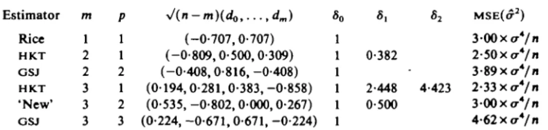
Table 1. Coefficients for equidistant design, relative weights of pth order divided differences and asymptotic mean squared error of some

difference-based estimators ..,dm) 50 5, S2 M S E ( ( ?2) Estimator Rice H K T GSJ H K T 'New' GSJ m 1 2 2 3 3 3 P 1 1 2 1 2 3 (-0-707, 0-707) (-0-809,0-500,0-309) (-0-408,0-816,-0-408) (0-194,0-281,0-383,-0-858) (0-535, -0-802, 0-000,0-267) (0-224, -0-671, 0-671, -0-224) 0-382 2-448 0-500 4-423 3-OOx a*/n 2-50 xa*/n 3-89x<74/n 2-33 x o -4/ " 3-00 x a*/n

Now for smoothness order p = 2 the question arises whether it is possible to improve the variance of the GSJ-estimator without essentially increasing the bias by going from

m = 2 to 3. While the idea of divided differences and of the GSJ-estimators is successive differencing, that of the HKT-estimators is to smooth normalized first-order differences yi+i-yt to improve the variance of the estimator. Indeed, for m = 2 the HKT-pseudo-residuals are

e, = ( « - 2 ) - * 0-809(1,0-3*2)iyl+l-y,,y,+2-yl+iy

(Table 1). To generalize this idea to general p and m = p+ 1 let us introduce 5,

1

a bidiagonal smoothing matrix of order (n - m) x (n - m +1). Then define general differen-ces of order m = p +1 for smoothness order p as

Let ^\m-p) be the rows of b{m-p). Then, pseudo-residuals e, = w,b\m-p)y can be defined as weighted general differences, such that (13) is fulfilled, and a1 is as in (2).

A generalization to arbitrary m>p is straightforward. Special cases are the OSJ-estimator for arbitrary p and m=p with 8 ^ 0 and the GSJ-OSJ-estimator for m = p + l with St = — 1. For equidistant design the HKT-estimator for m = 2 with p = 1 and 6, = 0-382 is a special case (Table 1).

The question is how to specify the weight 5,. A finite optimal 8, depends on the class of regression functions, sample size and design. Here, the asymptotic idea of Hall, Kay

Nonparametric estimation of residual variance 379 & Titterington (1990) proves to be useful. For p = 2, m=3 and equidistant design on [0,1] general differences (22) become

*?My = (n2/2)(l, - 2 + 5,, 1 - 2 5 , , 5,)(>-M . . . . yi+3)', and tr (A2) in (7) is minimal for

_35(n-3)-54 rf35(n-3)-54]

1*

1

28(n-3)-36 Ll28(n-3)-36J J "

For n-*oo this optimal value tends to 5, = (5±3)/4. Table 1 shows the estimator for 5, = 0-5. It is called 'new' and used in the case study in § 3. The other solution gives just the reflected difference.

Consider the class of difference-based estimators of order m = p +1 satisfying (12) for polynomials of order less than p. Arguments similar to Hall, Kay & Titterington (1990) show that the 'new' estimator is asymptotically optimal in this class under standard assumptions for regular designs, general error distributions and general regression func-tions. For an equidistant design we obtain

tr (A2new) = 3/{2(it - 3)} - 33/{49(n -3)2},

which leads to a relative gain in asymptotic variance of 23% relative to the GSj-estimator and a loss of 20% relative to the HKT-estimator for m =2; see Table 1.

3. A CASE STUDY

3-1. The design of the case study

The finite sample properties of the GSJ-, HKX- and 'new' estimators have been investi-gated using the formulae (4) and (5) and the explicit expressions (6)-(ll). All results for fixed designs are exact, and no simulations were necessary. After describing the situations considered the results are illustrated for some typical and interesting ones.

The regression functions considered were (i) linear: r(x) = 2x, (ii) exponential: r(x) = 2exp(-x/0-3), (iii) sine: r(x) = 2 sin (4TTX), and (iv) linear with Gaussian peak: r(x) = 2 - 5 x + exp{-100(x-0-5)2}. The results were compared for two residual variances (i)

a2 = 0-1 and (ii) a2 = 1. The sample size varied between 15 and 500. Four types of design on [0,1] were studied: (i) equidistant fixed design: x, = (i-0-5)/n, (ii) nonequidistant fixed design: x, are quantiles of a Beta (2, 2) distribution, (iii) random design: x, are uniformly distributed on [0,1], and (iv) random design: x, are distributed Beta (2,2). The error distributions were: (i) normal (y = 0, K = 0 ) , (ii) skewed (y = 1-155, K = 2): ^-distribution with 6 degrees of freedom, and (iii) platykurtic (y = 0, K =3): /-distribu-tion with 6 degrees of freedom.

3-2. Equidistant design and normal errors

For every situation, r(x), a2, n and design given, the finite optimal coefficient 5( for

general differences in (22) of order m = 2 for p = 1 was computed by grid search, and the relative inefficiencies of the HKT-, OSJ- and 'new' estimators relative to the resulting 'ideal' one were plotted: ineff ((72) = MSE(^2)/MSE(o2de,1).

For exponential and linear regression functions, asymptotics begin to work already at sample size n = 30. The HKT-estimator becomes then practically the optimal estimator of order m = 2. The GSJ-estimator achieves its asymptotic relative inefficiency of -£, and the

380 B. SEIFERT, T. GASSER AND A. WOLF 400 300 200 100 0-r\

1

1

1

I1

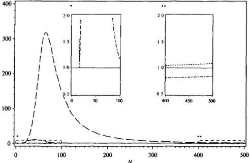
Fig. 1. Relative inefficiencies of the HKT- (long dashes), GSJ- (short dashes), and 'new' (dash-dot) estimators for sample size n = 15-500, sine regression function and a1 = 0-1.

Above are magnified windows for small (left) and large (right) sample size.

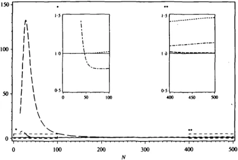
'new' estimator is a compromise, with relative inefficiency f. The situation changes dramatically for the sine function and o-2 = 0-l; see Fig. 1. The relative inefficiency of

the HKT-estimator achieves a value of 317 for n = 65, while the other estimators behave well over the whole range of sample sizes (compare the magnified windows in Fig. 1). For n = 200 observations the HKT-estimator has a relative inefficiency of 20. Even for n = 500 the asymptotic formula (19) does not correctly reflect the situation. There the HKT-estimator still has a relative inefficiency of more than 2, while the 'new' estimator is superefficient. The situation eases for higher noise to signal ratio. The regression function with a Gaussian peak (Fig. 2) gives similar results.

3-3. Other cases

The situation is comparable for regular nonequidistant fixed designs. The asymptotic bias, variance and mean squared error remain, but for small sample size the values may change. In the example of a nonequidistant design with n = 25, sine regression and normal errors with o-2 = 0-l, the mean squared error of the estimators is reduced by factors

3-5 (HKT), 9 (GSJ) and 11 ('new'). Table 2 shows the mean squared error for a moderate example. There changes are small for all error distributions.

The shape of the error distribution has no influence on the expectation of a difference-based estimator (compare (3)). The variance, however, changes; compare (4). The influence of skewness asymptotically is negligible and small for finite samples. As to the influence of kurtosis let us assume an equidistant design. Then, standard calculations using (8) yield

Consequently, the kurtosis of the error distribution heavily influences the variances of estimators, but for all estimators by nearly the same amount. A similar observation holds for nonequidistant designs (Table 2).

381 ISO 100 50-0 * * 1-5

j 1

j \

\

Fig. 2. Relative inefficiencies of the HKT- (long dashes), GSJ- (short dashes), and 'new' (dash-dot) estimators for sample size n = 15-500, linear regression function with Gaussian peak and o-2 = 0-l. Above are magnified windows for small (left) and large

(right) sample size.

Table 2. Mean squared error of estimators for sample size n = 100, sine regression function and oJ1=\ Design Equidistant Nonequidistant Random B(2, 2) Random U[0,1] Error distribution Normal Skewed Platykurtic Normal Skewed Platykurtic Normal Normal H K T 0086 0106 0116 0051 0-072 0081 0031 0032 MSE(<72) GSJ 0039 0060 0070 0040 0-060 0071 0041 0040 New 0031 0051 0062 0032 0053 0063 0050 0049

For random designs, the explicit formulae for finite sample mean squared error no longer work. In the study each case was simulated 400 times, and formulae

E(a2) = E{E(&2\x1,...,xn)},

var (<r2) = £{var ( < 72| x , , . . . , *„)} + E[{E(&2\x,,..., xn)}2]-{E(a2)}2

together with (4) and (5) were used to improve efficiency of simulations. The asymptotic mean squared error was the same for HKT- and GSJ-estimators as in the equidistant case. The asymptotic mean squared error of the 'new' estimator, however, increased by a factor of about 1-5; see Table 2.

3-4. Conclusions

The HKT-estimator should be used only for large sample sizes and flat regression functions. But many typical applications, for example biostatistical ones, have sample

sizes n = 15 to 100. The problems with bias for the HKT-estimator are in qualitative accordance with the smoothness assumption p = \. The 'new' estimator behaves well over a wide range of situations, but may be somewhat inefficient for small sample size and for irregular and random designs. The GSJ-estimator behaves well in all situations. Consequently, the GSJ-estimator is a reasonable compromise.

4. SOME GENERALIZATIONS 4-1. Random designs

The finite sample minimax property of the GSJ-estimator in Theorem 2 essentially remains for random designs. Let us discuss convenient assumptions. The class of regression functions now is restricted by (16) to 'smooth' ones. The n > p design points should be distinct with probability 1. Otherwise we can do better (§ 4-2). Some additional assumption on r(x) and/or the distribution of design points is needed to ensure a bounded mean squared error of the GSJ-estimator of order m = p. If we assume for simplicity that the pth derivative of the regression function is uniformly Lipschitz continuous and the design is on [0,1], no additional assumption is necessary.

THEOREM 3. Under the above assumptions, the GSJ-estimator of order m=p is the

essentially unique minimax estimator in the class of difference-based estimators (2) of order m^p satisfying (13) for almost all realizations of the design.

The proof goes along the lines of that of Theorem 2. As a consequence, the mean squared error of the Hicr-estimator is unbounded, while that of the GSJ- and 'new' estimators is bounded.

4-2. Multiple measurements

Multiple measurements are a chance for estimation of variance, for only in this situation is there an unbiased estimator. Gasser et al. (1986) and Hall, Kay & Titterington (1990) proceed as usual; others, e.g. Buckley et al. (1988), even exclude this situation. Assume observations yfj for j = 1 , . . . , n, s» 1 at different design points x, < . . . < xn. Let yt denote a cell mean and s1 the unbiased analysis-of-variance-estimator of a1. For normal errors,

s2 is independently distributed of any nonparametric estimator a2 based on yh Pseudo-residuals for yu can be computed as before. Condition (13) is replaced by 1 d]J nl+k =

\/{n-m). The mean squared error of a-2nix = as2 + (1 -a)a2 is minimized for a = MSE(<T2)/{MSE(S2) + MSE(<T2)}.

The gain over s2 and a2 can be considerable.

4*3. General weights

The choice of equal weights in (13) is the simplest but not necessarily the natural and optimal one. Several authors (Kendall, 1946, Problem 30.8; Quenouille, 1953; Anderson, 1971, pp. 73-) discussed corrections. One possibility is to use general weights 2 d\ = c, for i = 1 , . . . , n — m instead of (13) and find the optimal ones. For an equidistant design, GSJ-pseudo-residuals for m=2, and n = 10; e.g. we get the weights copt =

(0182,0080,0129,0-109, 0109,0129, 0080,0182). The gain of variance is 3% only. Since the gain is relatively small for the additional amount of work, we recommend the classical weights, at least for sample size ns» 10.

4-4. Multidimensional designs

Difference-based methods can easily be generalized to multidimensional designs. Important differences between the one- and higher-dimensional case are the very rich variety of configurations and the increasing portion of the boundary for growing dimension. In an as yet unpublished paper, E. Herrmann, M. P. Wand, J. Engel and T. Gasser generalized the GSj-estimator for m = 2 to the bivariate case. Hall, Kay & Titterington (1991) generalized the HKT-estimator to bivariate lattice designs and dis-cussed the problem of different configurations in detail. Further research has to be done to find optimal configurations.

REFERENCES

A N D E R S O N , O. (1929). Die Korrelationsrechnung in der Konjunkturforschung. Bonn: Schroeder. A N D E R S O N , T. W. (1971). The Statistical Analysis of Time Series. New York: Wiley.

D E BOOR, C. (1978). A Practical Guide to Splines. New York: Springer.

BUCKLEY, M. J. & EAGLESON, G. K. (1989). A graphical method for estimating the residual variance in nonparametric regression. Biometrika 76, 203-10.

BUCKLEY, M. J., E A G L E S O N , G. K. & SILVERMAN, B. W. (1988). The estimation of residual variance in nonparametric regression. Biometrika 75, 189-99.

CARTER, C. K. & EAGLESON, G. K, (1992). A comparison of variance estimators in nonparametric regression. /. R. Statist Soc B 54, 773-80.

CAVE-BROWNE-CAVE, F. E. (1904). On the influence of the time factor on the correlation between the barometric heights at stations more than 1000 miles apart. Proc R. Soc. London 74, 403-13.

E U B A N K , R. L. A S P I E G E L M A N , C. H. (1990). Testing the goodness of fit of a linear model via nonparametric regression techniques. J. Am. Statist. Assoc 85, 387-92.

GASSER, T., KNEIP, A. & KOHLER, W. (1991). A flexible and fast method for automatic smoothing. J. Am.

Statist. Assoc. 86, 643-52.

GASSER, T., SROKA, L. & J E N N E N - S T E I N M E T Z , C. (1986). Residual variance and residual pattern in nonlinear regression. Biometrika 73, 625-33.

HALL, P., KAY, J. W. & TITTERINGTON, D. M. (1990). Asymptotically optimal difference-based estimation of variance in nonparametric regression. Biometrika 77, 521-8.

HALL, P., KAY, i. W. & TITTERINGTON, D. M. (1991). On estimation of noise variance in two-dimensional signal processing. Adv. AppL Prob. 23, 476-95.

HALL, P. & M A R R O N , J. S. (1990). On variance estimation in nonparametric regression. Biometrika 77,415-19. HOOKER, R. H. (1905). On the correlation of successive observations, illustrated by corn prices. J. R. Statist.

Soc 68, 696-703.

K E N D A L L , M. G. (1946). The Advanced Theory of Statistics, 2. London: Griffin.

QUENOUILLE, M. H. (1953). Modifications to the variate-difference method. Biometrika 40, 383-408. RAO, C. R. & KLEFFE, J. (1988). Estimation of Variance Components and Applications. Amsterdam:

North-Holland.

RICE, J. (1984). Bandwidth choice for nonparametric kernel regression. Ann. Statist. 12, 1215-30.

SILVERMAN, B. W. (1985). Some aspects of the spline smoothing approach to nonparametric regression curve fitting (with discussion). J. R. Statist. Soc. B 47, 1-52.

" S T U D E N T " (1914). The elemination of spurious correlation due to position in time and space. Biometrika 10, 179-80.

THOMPSON, A. M., K A Y , J. W. & TITTERINGTON, D. M. (1991). Noise estimation in signal restoration using regularisation. Biometrika 78, 475-88.

TINTNER, G. (1940). The Variate Difference Method. Bloomington, Ind.: Principia Press.

WAHBA, G. (1983). Bayesian "confidence intervals" for the cross-validated smoothing spline. J. R. Statist.

Soc B 45, 133-50.