Radiation Monte Carlo approcah dedicated to the coupling with LES reactive simulation.

HAL Id: tel-00594229

https://tel.archives-ouvertes.fr/tel-00594229

Submitted on 4 Jul 2014

HAL is a multi-disciplinary open access archive for the deposit and dissemination of sci-entific research documents, whether they are pub-lished or not. The documents may come from teaching and research institutions in France or abroad, or from public or private research centers.

L’archive ouverte pluridisciplinaire HAL, est destinée au dépôt et à la diffusion de documents scientifiques de niveau recherche, publiés ou non, émanant des établissements d’enseignement et de recherche français ou étrangers, des laboratoires publics ou privés.

coupling with LES reactive simulation.

Jin Zhang

To cite this version:

Jin Zhang. Radiation Monte Carlo approcah dedicated to the coupling with LES reactive simulation.. Other. Ecole Centrale Paris, 2011. English. �NNT : 2011ECAP0011�. �tel-00594229�

THÈSE

présentée par

Jin ZHANG

pour l’obtention du

GRADE de DOCTEUR

Formation doctorale : Energétique

Laboratoire d’accueil : Laboratoire d’Energétique Moléculaire et Macroscopique, Combustion (EM2C) du CNRS et de l’ECP

Radiation Monte Carlo Approach

dedicated to the coupling with LES reactive simulation

Soutenue le 31 Janvier 2011

Composition du jury : M. Gokalp _{I. Président}

MMe. Eihafi M. Rapporteur

M. Dupoirieux F. Rapporteur

M. Gicquel O. Examinateur

M. Veynante D. Examinateur

Ecole Centrale des Arts et Manufactures Grand Etablissement sous tutelle du Ministère de l’Education Nationale Grande Voie des Vignes

92295 CHATENAY MALABRY Cedex Tél. : 33 (1) 41 13 10 00 (standard) Télex : 634 991 F EC PARIS

Laboratoire d’Energétique Moléculaire et Macroscopique, Combustion (E.M2.C.) UPR 288, CNRS et . . . cole Centrale Paris Tél. : 33 (1) 41 13 10 31

Télécopie : 33 (1) 47 02 80 35

J’adresse tout à bord un très grand merci à Messieurs Olivier Gicquel et Denis Veynante, qui m’ont accueilli au laboratoire EM2C pour effectuer ces travaux présentés et m’ont en-cadré pendant ma thèse, pour m’avoir fait profiter leurs connaissances scientifiques et leurs méthodes de recherches, pour leurs patiences, leurs disponibilités, leurs conseils pertinents, et surtout leurs soutiens à la fin de ma thèse.

Je remercie vivement Monsieur Jean Taine, professeur de l’Ecole Centrale Paris, qui m’a fait bénéficier de ses riches connaissances en transfert radiatif.

Je tiens à remercier sincèrement Madame Mouna EI Hafi, professeur de l’École des Mines d’Albi Carmaux, du Centre Energétique - Environnement, ainsi que Monsieur Francis Dupoirieux, ingénieur de recherche à l’ONERA, qui ont accepté de juger ce travail et d’en être les rapporteurs. Je remercie également à Monsieur Iskender Gökalp, directeur du Laboratoire CNRS de combustion et systèmes réactifs (LCSR) d’Orléans, qui m’a fait l’honneur d’avoir été président de mon jury de thèse.

Je remercie particulièrement Monsieur Lionel Tessé, ingénieur de recherche à l’ONERA, qui m’a beaucoup aidé dans la compréhension du code ASTRE et l’interprétation du principe réciproque de la méthode Monte Carlo.

Je remercie également Monsieur Gilles Grausseau, chercheur de l’IDRIS, qui m’a aidé à résoudre les problèmes informatiques quand j’ai fait les calculs parallèles chez IDRIS. Je souhaite aussi remercier à Rogério Gonçalves Dos Santos, docteur du laboratoire EM2C, ainsi que Kim Junhong, post-doc du laboratoire EM2C, avec qui j’ai travaillé sur le couplage combustion et rayonnement.

Je remercie à l’ensemble du personnel scientifique et administratif du laboratoire EM2C pour une très bonne ambiance.

Mes remerciements vont également à tous les thésards, docteurs et postdocs de notre labo-ratoire, pour les échanges fructueux que j’ai eus avec eux au cours de la thèse, spécialement pour Laetitia Pons, Jean-Michel Lamet, Nicolas Kahhali, Nicolas Tran et Yann Chalopin avec lesquels j’ai partagé le bureau.

Je souhaite enfin exprimer mes grands remerciements à mes parents qui ont toujours su me soutenir et m’encourager au cours de ma thèse.

Radiative transfer plays an important role in turbulent combustion and should be incorpo-rated in numerical simulations. However, as combustion and radiation are characterized by different time scales and different spatial and chemical treatments, and the complexity of the turbulent combustion flow, radiation effect is often neglected or roughly modelled. Coupling a large eddy simulation combustion solver and a radiation solver through a dedicated lan-guage CORBA is investigated. Four formulations of Monte Carlo method (Forward Method, Emission Reciprocity Method, Absorption Reciprocity Method and Optimized Reciprocity Method) employed to resolve RTE have been compared in a one-dimensional flame test case using three-dimensional calculation grids with absorbing and emitting medium in or-der to validate the Monte Carlo radiative solver and to choose the most efficient model for coupling. In order to improve the performance of Monte Carlo solver, two techniques have been developed. After that, a new code dedicated to adapt the coupling work has been proposed. Then results obtained using two different RTE solvers (Reciprocity Monte Carlo method and Discrete Ordinate Method) applied to a three-dimensional turbulent reacting flow stabilized downstream of a triangular flame holder with a correlated-k distribution model describing the real gas medium spectral radiative properties are compared not only in terms of physical behavior of the flame but also in computational performance (storage requirement, CPU time and parallelization efficiency). Finally, the impact of boundary con-ditions taking into account the actual wall emissivity and temperature has been discussed.

Résumé

Le transfert radiatif joue un rôle important en combustion turbulente et doit donc être pris en compte dans les simulations numériques. Toutefois, à cause du fait que la combus-tion et le rayonnement sont deux phénomènes physiques très différents caractérisés par des échelles de temps et d’espace également différentes, et la complexité des écoulements turbu-lents, l’effet du rayonnement est souvent négligé ou modélisé par des modèles très simples. Le couplage entre la combustion (LES) et le rayonnement avec l’environnement CORBA a été étudié. Dans le présent travail, quatre formulations de la méthode de Monte Carlo (méthode classique et méthode réciproque) dédiées à la résolution de l’équation de transfert radiatif ont été comparées sur un cas test de flamme 1D où l’on tient compte de l’absorption et de l’émission du milieu en utilisant un maillage 3D. Le but de ce cas test est de valider le solveur Monte Carlo et de choisir la méthode la plus efficace pour réaliser le couplage. Afin d’améliorer la performance du code de Monte Carlo, deux techniques ont été développées. De plus, un nouveau code dédié au couplage a été proposé. Ensuite, deux solveurs radi-atifs (Emission Reciprocity Monte Carlo Method et Discrete Ordinate Method), appliqués à une flamme turbulente stabilisée en aval d’un dièdre avec un modèle CK de propriétés radiatives, sont comparés non seulement en termes de description physique de la flamme, mais aussi en terme de performances de calcul (stockage, temps CPU et efficacité de la parallélisation). Enfin, l’impact de la condition limite a été discuté en prenant en compte l’émissivité et la température de paroi.

1 Introduction 1

1.1 Thesis background and application . . . 2

1.2 Thesis structure . . . 6

2 Numerical simulation of turbulent combustion 7 2.1 Conservation equations of turbulent combustion . . . 8

2.2 Choosing LES among different numerical approaches of turbulent combustion 9 2.2.1 Comparison of three turbulent numerical methods . . . 9

2.2.2 Bibliography for combining combustion and radiation study . . . 11

2.3 AVBP code . . . 12

2.3.1 Introduction . . . 12

2.3.2 Thickened Flame model for LES . . . 13

3 Numerical simulation of radiative heat transfer 15 3.1 Some basic concepts of radiative transfer applied in the turbulent combustion 16 3.1.1 Radiation monochromatic intensity . . . 16

3.1.2 Energy attenuation by absorption and out-scattering . . . 17

3.1.3 Energy gain by emission and in-scattering . . . 18

3.2 Radiative transfer equation . . . 19

3.3 RTE resolution methods . . . 21

3.3.1 Ray-tracing method . . . 22

3.3.2 Discrete ordinate method . . . 24

3.3.3 Monte-Carlo method . . . 26

3.3.4 Monte Carlo Numerical Scheme used in this thesis . . . 30

4 Monte Carlo numerical solver 37 4.1 Validation of Emission Reciprocal Monte-Carlo Method (ERM) with 1D flame using ASTRE . . . 38

4.1.1 Description of the test case . . . 38

4.1.2 Resultats and discussions . . . 41

4.1.3 Conclusions . . . 50

4.2 Improvement of ASTRE code’s performance . . . 52

4.2.1 "Grid merge" method . . . 53

4.2.2 "Near-range-interaction far-range-interaction" (NIFI) method . . . . 63

4.3 A new code "Rainier" . . . 78

4.3.1 Algorithms modified compared with ASTRE . . . 78

5 Comparison between DOM and Monte Carlo methods in large eddy

sim-ulation of turbulent combustion 83

5.1 Description of the test case ≪ Diedre_3D ≫ . . . 84

5.1.1 Experimental set-up and numerical configuration . . . 84

5.1.2 Combustion modeling with AVBP code . . . 85

5.1.3 Radiation modeling with "Rainer" code and "Domasium" code . . . . 86

5.2 Results and discussions . . . 88

5.2.1 Local convergence control . . . 88

5.2.2 Comparison with Domasium . . . 88

5.2.3 Conclusion . . . 90

6 Influence of the boundary condition in the numerical simulation of the radiative heat transfer coupled with turbulent combustion 93 6.1 Introduction of the boundary condition problem in radiative heat transfer . . 94

6.2 Flux calculation at the boundaries . . . 94

6.2.1 Flux computation notions used . . . 95

6.2.2 Results and discussions . . . 95

6.3 Comparison of radiative results with different boundary conditions . . . 101

6.3.1 Emissivity . . . 101

6.3.2 Wall temperature . . . 105

Conclusion 111 A Radiative properties model - CK model 115 A.1 Correlated-K model . . . 115

A.2 Frequency generation methods . . . 116

Introduction

Table of contents

1.1 Thesis background and application . . . 2 1.2 Thesis structure . . . 6

1.1

Thesis background and application

From an environmental point of view, nowadays the air pollution problem becomes more and more serious and attracts the whole world’s attention. As one of the main contributors of that, combustion processes are required to be better controlled to reduce the emission of the polluting products such as COx, NOx, soots etc. On the other hand, from an economical point of view, improving the combustion efficiency and performance is always the principal challenge that some related industries have to face, not only aeronautics but also for some energy industries. As a result of these two points, a high level knowledge about combustion processes and efficient tools to describe and resolve combustion systems as best as possible are then urgently required.

As combustion is a complex sequence which mixes chemical kinetics, thermodynamics and fluid dynamics, so its resolving and improvements need a better understanding and modeling of all the physical processes controlling a flame, such as turbulence, molecular physics and radiative heat transfer.

This thesis will be focused on the impact of the radiative heat transfer on turbulent com-bustion. The objective is to develop an efficient numerical tool of radiation simulation and to analyze the impact of the radiative heat transfer on turbulent combustion.

Reaction rates relevant to pollution products are known to be sensitive to the combus-tion temperature. So it is necessary to precisely estimate the local temperature, taking into account its fluctuations in the chemical kinetics calculations. Being a source term of the energy equation (volume radiative power), radiative heat transfer should be rigorously modeled to determine the temperature field with a high level of precision. The influence of the radiation on the combustion temperature and the polluted emission such as NOx and soots have been pointed out by some existing studies (De Lataillade 2001; Sivathanu and Gore 1994; Daguse 1996; Kaplan et al. 1994; Hall and Vranos 1994). Furthermore, radiative heat transfer plays a crucial role in the control of the charge heating in furnaces, in thermal heat losses and wall heat fluxes and in the control of the propagation of large scale fires. For example, Fig. 1.1, extracted from Goncalves Dos Santos et al. (2008), displaying a 2D flame structure and temperature (instantaneous field) and 1D cut temperature profiles from an average field, shows that on the one hand radiative heat transfer modifies the flame front structure with the maximum temperature decreased by heat losses and temperature gradients smoothed, and on the other hand the standard deviation is larger when radia-tion is taken into account which means that radiaradia-tion modifies the flame dynamics. The experimental setup used for this test is detailed in Chapter 5.

However, the fact that combustion and radiative heat transfer are two phenomena physi-cally different makes the coupling difficult. Usually combustion is focused on the balance

ation

(a) Instantaneous resolved temperature fields without (top) and with (bottom) radiative heat transfer. Spatial coordinates are given in m

!!!!!!"" #$%#&"&'# !!!!!!"" #%(&&#&"&'# ##################### #$%#&"()#

# # #%(&&#&"()#

(b) Transverse profiles of the temperature standard deviation at two downstream locations from the flame holder x = 7 cm and x = 16 cm without (NR) and with (NR100) radiative heat transfer.

Figure 1.1 – An example showing the influence of the radiation on the combustion temper-ature and the turbulent flame structure, a premixed propane/air flow is in-jected into a rectangular combustion chamber and a V-shape turbulent flame is stabilized behind the flame holder, the upstream mean velocity is about 5m.s−1

and the equivalence ratio φ = 1 is chosen (Goncalves Dos Santos et al. 2008).

over small volumes (finite volume framework) and radiative heat transfer involves long distances interaction as shown in Fig. 1.2. Therefore, two different numerical tools are

needed. Furthermore, solving Reynolds averaged Navier-Stokes (RANS) equations only

Combustion Balance over small volumes

Radiative heat transfers Long distance interactions

Figure 1.2 – Different scales of combustion and radiation in their numerical simulations gives access to some mean quantities such as mean temperature or mean species fractions at a given location, although if the probability density functions (PDF) model describing one-point statistics is involved, the local fluctuations of temperature and composition may be modeled. But unfortunately, radiative heat transfer is controlled by the distribution of cold and hot gases along optical paths, and radiative power is highly nonlinear and varies directly with the fourth power of the local instantaneous temperature, which requires in-formation on spatial correlations usually not available in RANS. Then other Navier-Stokes solving methods which asks for more CPU time like LES or DNS should be applied here. On the other hand, most of the radiative transfer equation resolution approaches such as Ray-tracing technique, Discrete Ordinate Method and Monte Carlo Simulation are always very expensive in terms of CPU time requirement and memory storage. Consequently, the challenge is to find a compromise between taking into account the radiative heat transfer as precisely as possible and reducing the computational requirement in terms of CPU time and memory.

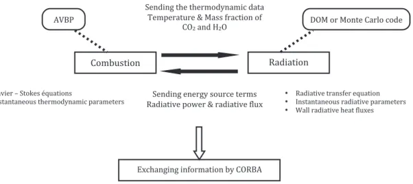
After referring to some existing researches about combustion numerical simulations includ-ing radiation and other physical phenomena such as turbulence and chemistry with different levels of simplifications and assumptions because of limited computational resources (bib-liography being presented in Section. 2.2.2), a numerical approach developed in the Phd. thesis of Goncalves Dos Santos (2008) will be used here to couple turbulent combustion and radiative heat transfer considering the turbulence/radiation interaction (TRI), non-gray medium with detailed radiative gases properties modeled and "industrial" configura-tions (three dimensional heavy mesh), furthermore taking into account the computational resources limits. This approach is based on two independent solvers linked through a spe-cialized framework, CORBA - Common Object Request Broker Architecture (Henning and Vinoski 1999), dedicated to couple two solvers and taking advantages of different charac-teristic time of each phenomenon. Fig. 1.3 displays the coupling principe:

• CORBA allows construction of applications constituted of software modules that exchange information over a network. It works through internet protocols and distant machines or/and different platforms can be used.

informa-tion (radiative flux and energy source terms) and the radiainforma-tion code (server) sends the information back. Then the combustion code also sends its output data (thermo-dynamic data such as temperature and mass fraction) to the radiation code.

• The combustion code used here is AVBP code and the radiation code can be Discrete Ordinate Method (DOM) code or Monte Carlo Method code.

By using this tool, Goncalves Dos Santos has coupled a LES solver AVBP developed by CERFACS and IFP (Schoenfeld 2008) with a three-dimensional discrete ordinate method (DOM) solver (Goncalves Dos Santos 2008).

! "#$%&'()#*! +,-),()#*! ./*-)*0!(1/!(1/2$#-3*,$)4!-,(,! 5/$6/2,(&2/!7!8,''!92,4()#*!#9! ":;!,*-!<;:! ./*-)*0!/*/203!'#&24/!(/2$'!! +,-),()=/!6#>/2!7!2,-),()=/!9?&@! • A,=)/2!B!.(#C/'!DE&,()#*'!

• F*'(,*(,*/#&'!(1/2$#-3*,$)4!6,2,$/(/2'! • +,-),()=/!(2,*'9/2!/E&,()#*!• F*'(,*(,*/#&'!2,-),()=/!6,2,$/(/2'! • G,??!2,-),()=/!1/,(!9?&@/'!

HIJK! L:8!#2!8#*(/!",2?#!4#-/!

M@41,*0)*0!)*9#2$,()#*!%3!":+JH!

Figure 1.3 – Coupling principe between two parallel solvers dedicated to turbulent combus-tion (AVBP) and radiative heat transfer (DOM or Monte Carlo Method) by using CORBA framework

In the precedent paragraph, the numerical coupling tool (CORBA) has been described. In this part, the two numerical solvers respectively for turbulent combustion and radiation will be briefly presented. On the one hand, a stochastic Monte Carlo method is used to solve radiative transfer. Compared with deterministic methods such as DOM, SHM -Spherical Harmonics Method (Mazumder and Modest 1999), Monte Carlo does not need some simplifying assumptions, i.e. optically thin fluctuation assumption (OTFA) and gas radiative properties assumptions (i.e. reducing the spectral bands number). Therefore, a much more precise result will be obtained with Monte Carlo. More details about the advantages of this method will be presented in Chapter 3.3.3. On the other hand, AVBP code is retained as the LES solver.

In the first part of this thesis, a code called ASTRE (Approche Statistiques des Transferts Radiatifs dans les Ecoulements), developed by Tessé during his Phd. thesis (Tesse 2001), is used here as Monte Carlo solver. ASTRE can deal with complex three-dimensional geome-tries taking into account the non-isothermal and heterogeneous non-gray medium, a detailed spectral discretization of the radiative gases properties and a diverse direction presentation of the particles, turbulence/radiation interaction and radiative non-isotope diffusion of the particles. Furthermore, this code uses three reciprocal Monte Carlo formulations and one forward Monte Carlo formulation at the same time (Tesse et al. 2002). The first task of this thesis is to compare these four formulations on a one-dimensional flame application to

find the most suitable formulation for coupling in terms of the precision and computational requirements.

After several tests, we found that when ASTRE code is applied to a complex geometry (i.e. a mesh with 3.4 million cells), if a detailed radiative gases properties model is needed (i.e. Correlated-k model with 1022 spectral bands), the memory storage required might become very huge (detailed figure will be presented in Chapter 4 ) and might not be acceptable by usual scientific computers. As a result of that, two techniques have been developed to improve the performance of ASTRE code in terms of computational CPU time and storage requirements to facilitate the coupling work when applied to a complex real industrial geometry and taking into account a detailed radiative gases properties such as correlated-k model. Then, a new parallel code based on ASTRE and dedicated only to the coupling with turbulent combustion has been developed. It can be considered as a subroutine of ASTRE which is easier to be coupled with other codes.

Boundary conditions are often simplified in radiation/combustion interaction problems. But in fact, their influence on wall radiative fluxes and radiative power in the medium cannot be neglected. So the impact of boundary conditions will be discussed at the end of this thesis taking into account the effects of actual wall emissivity, temperature and convection phenomena.

1.2

Thesis structure

This manuscript emphasizes the specific problems linked to the development of an efficient Monte Carlo solver, requiring less computational resources and to be applied easily to industrial configurations, for Large Eddy Simulation of turbulent combustion including radiative heat transfer. The scope of this thesis is listed below:

• Chapter 2: Basic presentation and comparison of different turbulent combustion modeling methods, explaining LES model is chosen for this work and presentation of turbulent combustion solver being used here - AVBP code.

• Chapter 3: Basic concepts of radiative heat transfer and a brief presentation about the different methods for radiative transfer equation resolution, particularly focused on the Monte Carlo method and explaining its advantages, finally emphasizing the Monte Carlo numerical scheme being used in this thesis.

• Chapter 4: Emission Reciprocal Monte Carlo Method (ERM) has been validated applied on a 1D flame by using ASTRE and chosen as the most suitable model for coupling. Two techniques have been developed to improve the performance of ASTRE code, which are respectively "Grid merge" method and "near/far-range-interaction" model. Finally, a new code only using ERM model dedicated to the coupling had been developed from ASTRE.

• Chapter 5: Discrete Ordinate Method (DOM) and Monte Carlo Method applied to a three-dimentional flame have been compared in terms of physical behavior and computational performances.

• Chapter 6: The influence of boundary conditions has been discussed taking into account the impact of wall emissivities and wall convection phenomena.

Numerical simulation of turbulent

combustion

Table of contents

2.1 Conservation equations of turbulent combustion . . . 8 2.2 Choosing LES among different numerical approaches of

tur-bulent combustion . . . 9 2.2.1 Comparison of three turbulent numerical methods . . . 9 2.2.2 Bibliography for combining combustion and radiation study . . . 11 2.3 AVBP code . . . 12 2.3.1 Introduction . . . 12 2.3.2 Thickened Flame model for LES . . . 13

In this chapter, the basic balance equations used in turbulent combustion studies are firstly introduced, then a comparison between the different numerical methods is presented to evidence the choice of LES method for the study. Finally, the numerical tool AVBP -used here is briefly described.

2.1

Conservation equations of turbulent combustion

The basic instantaneous local balance equations to describe combustion can be summarized using the classical lettering as below (Barrere and Prud’homme 1973; Williams 1985; Kuo 1986; Poinsot and Veynante 2005):

Mass conservation (j=1,2,3): ∂ρ ∂t + ∂ρuj ∂xj = 0 (2.1)

where ρ is the density of the mixture, uj is the j component of the velocity vector u.

Momentum conservation (i=1,2,3): ∂ρui ∂t + ∂ρujui ∂xj = −∂p ∂xi +∂τij ∂xj + Fi (2.2)

where τij is the viscous tensor and Fi is a body force (such as gravity, etc). For Newtonian

fluids, according to the Newton law, the viscous tensor is written as: τij = µl  ∂ui ∂xj + ∂uj ∂xi − 2 3µlδij  ∂uk ∂xk (2.3)

where µl is the shear viscosity and δij is the Kronecker symbol.

Species conservation (N species with k = 1, · · · , N ):

∂ρYk ∂t + ∂ρujYk ∂xj = −∂J k j ∂xi + ˙ωk (2.4) where Jk

j is the molecular diffusive flux of species k in direction j and ˙ωk is the mass

reaction rate of the species k per unit volume. These species molecular diffusivities Jk

j can

be described using the Fick’s law as: J_jk= − µl

Sck

∂Yk

∂xj

where Sck, the Schmidt number of the species k, is defined as:

Sck=

µl

ρDk

(2.6)

Dk is the molecular diffusivity of the species k relatively to the major species.

Total enthalpy (ht= h + uiui/2) ∂ρht ∂t + ∂ρujht ∂xj = ∂p ∂t + ∂ ∂xj (J_jh+ uiτij) + ujFj (2.7)

where uiτij and ujFj are respectively the power due to the viscous and body forces. The

enthalpy diffusion Jh

j can be described as:

Jjh = − µl P r  ∂h ∂xj + n k=1 ! Pr Sck −1 " hk ∂Yk ∂xj # + Qr (2.8)

The Prandtl number Pr contains the diffusive transport of the momentum and temperature.

In this expression, the Dufour effect (enthalpy diffusion under mass fraction gradients) is

neglected. The Lewis number Lek of the species k representing the ratio between the

thermal and mass diffusivities can be introduced as:

Lek =

Sck

Pr

(2.9)

Qris the radiative power, it can be neglected or estimated from simplified radiative models.

Another possibility is to be calculated by a dedicated radiative solver using more accurate models as in the present thesis.

2.2

Choosing LES among different numerical approaches

of turbulent combustion

In this section, three numerical methods used to resolve the turbulent combustion problems are firstly introduced and compared. Then references focusing on the combining turbulent combustion and radiation studies are discussed. Based on the two previous parts, finally combustion solver with LES model is chosen to be used for this thesis.

2.2.1

Comparison of three turbulent numerical methods

In order to solve the balance equations mentioned above, some numerical methods have been developed. The principle of three turbulent numerical methods can be illustrated by the turbulent kinetic energy spectrum in figure 2.1.

Direct Numerical Simulation (DNS) offers the full numerical solution of the instantaneous balance equations for all of the spatial frequencies in the spectrum. All turbulence scales are explicitly determined without any model for turbulent motions (Poinsot and Veynante 2005). However, limited by the computational performance, this method can only be used

! "#$%! ! $&! '()*+,)!-./)0)/!12!3'45! 61*)&708!91-:0+7)/!12!3'45! 61*)&708!91-:0+7)/!12!;"5! ;+*,)!9&+0)! <./)0)/!12!;"5!5-+00!9&+0)!

Figure 2.1 – Turbulence kinetic energy spectrum plotted as a function of the inverse length scale (proportional to the wave number). RANS, LES and DNS are summa-rized in terms of spatial frequency ranges

for some very simplified cases (Poinsot 1996; Poinsot et al. 1996; Vervisch and Poinsot 1998), where time and length scale ranges present in the flow are very limited (small Reynolds numbers).

Reynolds-average Navier-Stokes (RANS) methods describe the mean flow field by averag-ing the balance equations. The local fluctuations and turbulent structures are integrated and presented as mean quantities form (such as mean temperature, mean mass fraction

of CO2 and H2O) directly linked to the probability to find hot burnt gases at a given

lo-cation (Poinsot and Veynante 2005). So the averaging operator in RANS is "temporal" (average in time) not "spatial". However, for combining turbulent combustion and radia-tion studies, radiative transfer is controlled by the instantaneous distriburadia-tion of cold and hot gases along optical paths which can not be directly extracted from mean flow character-istics. Probability density functions (PDF) may be introduced to overcome this problem, but PDF based methods can hardly take into account the spatial correlations which is cru-cial in radiative transfer. This turbulence-radiation interaction problem has been addressed by several authors (Giordano and Lentini 2001; Coelho et al. 2003; Li and Modest 2003). Large Eddy Simulation (LES) resolves explicitly the large flow structures (a cut-off scale is needed here, it can be chosen as the computational mesh size in some practical cases) and the effects of the structures smaller than the cut-off length scale are modeled. The major difference between RANS and LES comes from the operator employed in the deriva-tion (Goncalves Dos Santos 2008). As menderiva-tioned in the previous paragraph, in RANS, the averaging operator is applied over a set of realizations during a time scale. In LES, the operator is a spatial filter localized at a given size ∆, which is independent on time and applied to a single realization of the studied flow. So in the combining radiation and combustion studies, Large Eddy Simulation (LES) can give access to the instantaneous spatial distribution of fresh and burnt gases at the resolved scale levels (DNS also has this advantage).

A few words about LES equations. In LES, the quantities Q are filtered in the spectral space (cut-off filter) or in the physical space (weighted average in a given volume, box filter or Gaussian filter),the filter operation is defined as:

¯ Q(x) =



Q(x∗_{)F (x − x}∗_)dx∗ _(2.10)

where F is the LES filter: 

F (x)dx = 1 (2.11)

In reactive flows, a mass-weighted Favre filtering is introduced as (Poinsot and Veynante 2005):

¯

ρ ˜Q(x) = 

ρQ(x∗_{)F (x − x}∗_)dx∗ _(2.12)

Then the instantaneous balance equations in Chapter 2.1 can be filtered to derived

bal-ance equations for the filtered quantities ¯Q or ˜Q. Furthermore, any quantity Q may be

decomposed into a filtered component ¯Q and a "fluctuating" component Q′ _{written as:}

Q = ¯Q + Q′ _(2.13)

where Q′ _{represents the instantaneous fluctuations relative to the resolved field. More}

details about the LES filtered balance equations can be found in Poinsot and Veynante (2005).

2.2.2

Bibliography for combining combustion and radiation study

In combining combustion and radiation study domain, some researches have been realized. Laminar flame

Some studies focus on the laminar flame or neglect the effects of turbulent fluctuations for turbulent flame in order to understand the interactions between radiation and chemistry in combustion. De Lataillade (2001) has calculated a 1D counter flow laminar diffusion flame of methane by using a radiative Monte Carlo method with soot particles and radiative gases properties modeled by a statistical narrow band model formulated in k-distribution. Sivathanu and Gore (1994) have pointed out the strong coupling between soot formation and radiation in laminar acetylene diffusion flames by a ray-tracing radiative method with gray soot particles assumption. Liu et al. (2004) have performed a detailed calculation of an axisymmetric coflow laminar methane/air diffusion flame by using the Discrete Ordinate Method (DOM) and different implementations of the SNBCK-based band models with detailed gas-phase chemistry and soot modeled by an acetylene-based semi-empirical two-equation model. Zhu and Gore (2005) have simulated a one-dimension opposed-flow laminar methane/air diffusion flames with detailed gas chemistry and global soot kinetics using the Sandia OPPDIF code.

In turbulent flames, turbulence/radiation interactions, called TRI has to be considered. TRI arises from highly nonlinear coupling between temperature and composition fluctuations in both non-reacting and reacting turbulent flows. Faeth and Gore have concluded that TRI effect on the radiative transfer is very important (about 50-300% of the value without TRI effect), especially in turbulent diffusion flame of ethylene, acetylene and hydrogen (Gore et al. 1987; Gore and Faeth 1988; Kounalakis et al. 1988). As mentioned in precedent section, RANS modeling approaches are not well suited to dealing with TRI, then statistical approaches such as probability density function (PDF) methods are needed (Coelho et al. 2003; Li and Modest 2002). Adams and Smith (1995) have used a Discrete Ordinate Method (DOM) associated with the optically thin fluctuation assumption (OTFA or called self-absorption neglected) in an industrial furnace, assumed to be a gray medium. And the fluctuations of the thermo-physical properties have been deduced from a 2D PDF of the mixture ratio and of the total enthalpy.

DNS was combined with DOM (Discrete Ordinate Method) to investigate two dimension sooting flames for fires (Yoo et al. 2005). Wu et al. (2005) have implemented a photon Monte Carlo method for the solution of the radiative transfer equation in a turbulent combustion DNS code to study the turbulence-radiation interaction. However DNS computations still remain out of reach of practical industrial configurations in terms of CPU cost. Then LES appears as a very efficient alternative tool to deal with turbulent combustion radiation interaction. Indeed this approach can be expected to provide a more accurate representation of one-point statistics and spatial correlations, a key point when dealing with radiation. The combination of LES and DOM has been performed by several authors including the consideration of soot formation and radiation (Desjardin and Frankel 1999; Jones and Paul 2005). Additionally, Gonçalves Dos Sandos has performed a simulation coupling LES and DOM solvers through a specialized framework CORBA (Goncalves Dos Santos 2008; Goncalves Dos Santos et al. 2008). His results will be used later on in this thesis.

To conclude, combining work of turbulent combustion solvers (DNS, RANS, LES) and ra-diative transfer solvers (DOM, Monte Carlo, etc.) has been widely performed by using different combination couple. However, due to the computational resource limit, The cou-pling work between LES and Monte Carlo, which can give a satisfying results in terms of precision, has not been really realized, especially for the complex configurations. That is the reason why this thesis will focus on this coupling and show its feasibility.

2.3

AVBP code

2.3.1

Introduction

The LES solver used in this work is AVBP code (Selle et al. 2004) developed by CER-FACS and IFP and dedicated to compute reactive flows. It can resolve three dimensional compressible equations on structured and unstructured meshes. This solver is based on the finite volume or finite element methods with artificial viscosity sensor and explicit time integration.

The numerical schemes implemented "Lax-Wendroff scheme" (Hirsch 1989) is used for this thesis. It uses a second order Runge-Kutta time integration and central second order

spatial discretization. Compared with the other scheme of AVBP - TTGC scheme (Colin and Rudgyard 2000), Lax-Wendroff scheme is more feasible to be used for reacting flows and runs almost two times faster.

The NSCBC (Poinsot and Lele 1992) and wall law boundary conditions (Schmitt 2005) are used here. This code is parallelized by domain splitting using MPI library, a convenient approach for small volumes solving.

Finally, one of the reasons to choose this code for coupling is that its efficiency well adapted to the massive computation.

2.3.2

Thickened Flame model for LES

A difficult problem encountered for Large Eddy Simulation of premixed flames is that the thickness δ0

Lof a premixed flame (usually between 0.1 mm to 1 mm) is generally smaller

than the standard computational mesh size ∆ used for LES. Therefore, some models should be applied to resolve the flame fronts on a LES mesh (Poinsot and Veynante 2005).

The Thickened Flame model (TFLES) is used in this thesis to describe the premixed com-bustion. In this model, an artificial factor F has been introduced to thicken the flame front in order to resolve the front structure on LES numerical mesh. It is shown that multiplying species and heat diffusion coefficients by a factor F (i.e. the molecular diffusivity of the species D becomes F D) and decreasing the exponential constant by the same factor F (A is replaced by A/F, where A is the exponential constant for the reaction rate ˙ω) provides a flame propagating at the same laminar flame speed as the non-thickened flame, with its

thickness increasing as F δ0

l (Butler and O’Rourke 1977; Colin et al. 2000).

Additionally, this factor F will change the Damkohler number Da which characterizes the

ratio between the turbulent (τt) and the chemical (τc) time scales:

Da=

τ_t

τ_c (2.14)

the turbulent scale can be estimated from turbulent integral scale characteristics (τt= lt/u′,

where lt is the turbulence integral length scale and u′ is the velocity fluctuation related to

the square root of the turbulent kinetic energy) and the chemical time scale τc may be

estimated as the ratio of the thickness δL and the propagation speed SL of the laminar

flame. So the Damkohler number Da becomes:

Da= τ_t τ_c = lt δ_L SL u′ (2.15)

If the thickness δ is multiplied by the factor F , Dawill be divided by F . This low Damkohler

number corresponds to a slow chemical reaction. Reactants and products are mixed by turbulent structures before reaction (Poinsot and Veynante 2005). This point might impact the results of coupling work between combustion and radiation.

Later in the chapter 4, the impact of TFLES model with different artificial factors on the radiative results will be discussed.

Numerical simulation of radiative heat

transfer

Table of contents

3.1 Some basic concepts of radiative transfer applied in the tur-bulent combustion . . . 16 3.1.1 Radiation monochromatic intensity . . . 16 3.1.2 Energy attenuation by absorption and out-scattering . . . 17 3.1.3 Energy gain by emission and in-scattering . . . 18 3.2 Radiative transfer equation . . . 19 3.3 RTE resolution methods . . . 21 3.3.1 Ray-tracing method . . . 22 3.3.2 Discrete ordinate method . . . 24 3.3.3 Monte-Carlo method . . . 26 introduction . . . 26 Reciprocal Monte-Carlo method . . . 27 3.3.4 Monte Carlo Numerical Scheme used in this thesis . . . 30

3.1

Some basic concepts of radiative transfer applied in

the turbulent combustion

A flame is a medium that can absorb, emit and scatter radiation to transfer energy, and may also contain solid or liquid particles. Two difficulties could arise in studying radiation problems in combusting medium. Firstly, absorption, emission and scattering of energy occur not only at system boundaries, but at all locations in the medium. Then the temper-ature, radiation intensity and physical properties at every point will be required to describe energy exchanges in detail. The second difficulty is that spectral effects are often much more pronounced in gases than for solid surfaces, and a detailed spectrally dependent analysis may be required.

In this chapter, firstly, some fundamental concepts are introduced for radiant intensity within a medium, and for the effects of absorption, emission, and scattering on radiant propagation. Then the radiative transfer equation is formulated and some of its solution methods are described briefly. Finally, Monte Carlo method is detailed, together with the numerical scheme used in this thesis.

3.1.1

Radiation monochromatic intensity

The radiation monochromatic intensity Lν(r, ∆) (W · m

−2

· sr−1

· Hz−1

) is introduced in problems dealing with radiative transfer through absorbing, emitting and scattering medium. It can be defined as the radiation energy crossing through an area per unit time dt, per unit surface dS, per unit solid angle dΩ for the spectral frequency ν (Modest 2003; Taine et al. 2003): Lν(r, ∆) = d5_Φ ν(r, ∆) dΩ[dS · (∆ · n)]dν (3.1) where d5_Φ

ν(r, ∆) is the monochromatic energy flux (Watts) from a point of the space P (r),

crossing the surface dS (n is the normal direction of the surface dS and ∆ is the radiative

ray direction) in a solid angle dΩ, see Fig. 3.1.

To resolve the radiative transfer problem is then to determine the radiative monochromatic intensity. In consequence, a radiative transfer equation should be established for a given optical path and a given frequency (Tesse 2001).

"

n

d

"

Figure 3.1 – Radiative intensity

3.1.2

Energy attenuation by absorption and out-scattering

An optical beam carrying the spectral radiation intensity L′

ν crosses a participating medium

of thickness ds as shown in Fig. 3.2, the energy absorbed and scattered by this medium d6_Φ′a,s−

ν (s)

1_{depends on the magnitude of the incident intensity L}′

ν, the optical path distance

ds and an extinction coefficient βν of the medium which is a function of the temperature,

pressure, frequency of the incident radiation and characteristics of the medium. d6Φ′a,s−

ν (s) = −βνL

′

νdSdsdΩdν (3.2)

and the extinction coefficient can be represented as:

βν = κν+ σν (3.3)

where κν (∼ m−1) and σν (∼ m−1) are respectively the absorption coefficient and the

scattering coefficient. Absorption

Considering only the energy attenuated by the absorption, Eq. 3.2 can be written as an integration form over a optical path s = l:

d5Φ′a ν(l) = exp  − l 0 κνds  · d5Φ′ ν(0) (3.4) where d5_Φ′

ν(0) is the incident flux at s = 0 and δν =

l

0κνds is the optical thickness

(for the absorption) of the layer of thickness l and is a function of all the values of κν

between 0 and l. If δν ≫1, the medium is called optically thick, which means the mean

penetration distance is quite small compared to the characteristic dimension of the medium. For this condition, the thermal energy can be completely absorbed in a short distance, and a volume element within the material is only influenced by the surrounding neighboring

elements. If δν ≪ 1, the medium is then called optically thin, which means that the

1

!

*!+%)*%,!

"-!

"--!

"!

./%&01012$&'012$&' "#$%%$&' (()* %$&' "# "#$%%$%$

*(!

Figure 3.2 – Radiative energy evolution along an optical path

mean penetration distance is much larger than the medium dimension. Radiation travels entirely through the material without significant absorption and each element within the medium interacts directly with the medium boundary (Siegel and Howell 1981). In this thesis, without specific comments, the medium will be implicitly considered as "optically thin".

Out-Scattering

The radiation scattering represents the optical path deviation because of the interaction between a photon and another or more other particles during which the photon does not lose its entire energy. If the energy is attenuated by scattering, it will be called "out-scattering". Similar to the absorption, it can be written as:

d5Φ′s− ν (l) = exp  − l 0 σνds ! · d5Φ′ ν(0) (3.5)

3.1.3

Energy gain by emission and in-scattering

Emission

To maintain the local thermodynamic equilibrium in the computational domain (ex: the volume from S to S + ds presented in Fig. 3.2), all of the medium absorbing an amount of

energy can emit at the same time. d6_Φ′e

ν(s) representing the amount of energy emitted over

a certain path s that escapes into a given direction can be written as (Taine et al. 2003): d6Φ′e

ν(s) = ην(s)dSdsdΩdν = κνn

2_L◦

ν(Ts)dSdsdΩdν (3.6)

where ην(s) is the monochromatic emission coefficient. Under the local thermodynamic

equilibrium assumption, the absorbed flux is equal to the emitted one. So ην(s) = κνn

2_L◦ ν(Ts)

with n is the simple refractive index. L◦

ν(T ) is the blackbody intensity and it depends on

temperature T and frequency ν (only the spontaneous emission is taken into account here and the induced emission is neglected).

In particular, a engineering parameter "emissivity" (ε′

ν) has been defined to characterize

the radiation emission ability of an isothermal medium compared with the emission from a

blackbody at the same temperature2 _{(Taine et al. 2003):}

ε′ ν = 1 − exp(−κνl) = α ′ ν = 1 − τ ′ ν (3.7) where α′

ν is the absorptivity defining the absorption ability of a medium that determines

the fraction of radiant energy traveling along a path that will be absorbed within a given

distance and τ′

ν is the transmissivity defining the transmission ability of a medium that

determines the fraction of energy at the origin of a path that will be transmitted through a given thickness (Siegel and Howell 1981).

In-scattering

Different from the "out-scattering" mentioned above, the "in-scattering" defines the energy gained by the scattering. The scattered energy produced by an optical path in the direction

of u′ _{obtained by another optical path in the direction u can be represented as:}

d6Φs+ν = σν 4πdsdSdΩdν  4π 0 Pν(&∆′ → & ∆)L′ ν(&∆ ′_)dΩ′ _(3.8)

where a phase function Pν(&∆′ →

&

∆) has been introduced to describe the angular distribution

of the scattered energy, and the probability of the optical path from the direction &∆′

scattered into another direction &∆ is (dΩ/4π)Pν(&∆′ →

& ∆).

3.2

Radiative transfer equation

As shown in Fig. 3.2, the radiation energy traveling in an optical path from s to s + ds is decreased by absorption and out-scattering and is enhanced by the spontaneous emission and in-scatttering. Using the equations discussed above (Eqs. 3.2, 3.6 and 3.8), a first-order integral-differential equation, radiative transfer equation (RTE) is developed to describe the

radiation intensity along a path of ds long in the direction &∆.

d6_Φ′ ν dsdSdΩdν = −[κν(s) + σν(s)]L ′ ν(s, &∆) !" #

attenuation: absorption + out-scattering

+ κν(s)n 2_{(s, &∆)L}◦ ν(Ts) !" # gain by emission + σν 4π  4π 0 Pν(s, &∆′ → & ∆)L′ ν(s, &∆′)dΩ ′ !" # gain by in-scattering (3.9)

With the definition of radiation intensity, Eq. (3.9) can be rewritten as: n2(s, &∆) d ds $ L′ ν n2[s, &∆] % = −[κν(s) + σν(s)]L ′ ν(s, &∆) + κν(s)n 2_{(s, &} ∆)L◦ ν(Ts) + σν 4π  4π 0 Pν(s, &∆′ → & ∆)L′ ν(s, &∆′)dΩ ′ _(3.10) 2

The unsteady time term ∂/∂t contained in the first term d/ds is generally neglected because radiation propagation can be considered infinitely fast in usual cases.

For no-scatting medium, σν = 0, Eq. (3.10) can be integrated in the interval [0, s] and

written as (Taine et al. 2003): L′ ν n2(s, !∆) = L′ ν n2(0, ∆)τν(0 → s) +  s 0 κν(s′)L 0 ν(T (s ′_))τ ν(s′ →s)ds′ = L ′ ν n2(0, ∆)τν(0 → s) +  s 0 L0ν(T (s ′₎₎∂τν(s′ →s) ∂s′ ds ′ _(3.11)

where the first term represents the energy transmitted from 0 to s based on the incident intensity at s = 0 and the second term represents the energy emitted by each element

s′ _{between 0 and s and the transmission of this energy from s}′ _{to s. τ}

ν(s′ → s) is the

monochromatic transmissivity from s′ _{to s:}

τν(s ′ _{→s) = exp}  s s′ −_κν(s ′′_)ds′′ ! (3.12) and "_ss′κν(s′′)ds′′ represents the optical thickness between s′ and s.

Radiative heat flux

In general, the radiative heat flux ΦR _{is one of the most useful radiation quantities in}

engineering applications. Considering the radiative energy conservation in a volume element

V with the closure G around as shown in Fig. 3.3, the radiative volume power PR_(G)(W/m3₎

and the surface radiative flux φR _(W/m2_{) can be represented as (Tesse 2001):}

 #$%& volume PR(G)dV + ' #$%& surface φR(F )dS = 0 (3.13)

where dS corresponds to the surface area of the closure G and F is the departure point of

the optical path on the closure G. Using the radiation flux vector qR _{and the divergence of}

the radiative heat flux (∇_{· q}R_{), the integration of the surface radiative flux on G can be}

written as: ' #$%& surface φR(F )dS = ' #$%& surface −_{n · q}R_{(F )dS =}  #$%& volume [∇_{· q}R_{]s=GdV (3.14)}

And n is the normal direction of the surface G on the point F. Combining with Eq. (3.13) and Eq. (3.10) and neglecting the scattering, we have:

PR(G) = −[∇_{· q}R_{]s=G= −}  ∞ 0  #$%& 4π ∂Lν(s, ∆) ∂s ! s=G dΩdν =  ∞ 0  #$%& 4π κν(G)L ′ ν(G, ∆)dΩdν # $% & absorption −_4π  ∞ 0 κν(G)L 0 ν(TG)dν # $% & emission (3.15)

! "! #$! %! n #&! &!

Figure 3.3 – Flux calculated on a surface dS of the closure G

In this thesis, this term is calculated by the radiation solver and will be sent to the com-bustion LES solver as the radiative source term.

Boundary conditions problem

To obtain the solution of Eq. (3.9), the integration constant corresponding to the intensity at the departure point of the optical path must be determined. Because most of these departure points are usually at the boundary of the radiating medium, so the radiation at the boundaries should be taken into account and coupled with the radiation distribution inside the medium (Siegel and Howell 1981). For this reason, the influence of the bound-ary condition for the radiative problem can not be neglected. However, limited by the computational source and the boundary material property complexities, simplified models usually are used for boundary simulating. A more detailed discussion about the boundary condition problem will be offered in this thesis in Chapter 6.

3.3

RTE resolution methods

Several resolution methods of the radiative transfer equation are presented in this section. Firstly, the ray-tracing method will be shortly introduced, because from a certain point of view, its principle is close to Monte Carlo method which can be considered as its statistical variant. Then the Discrete Ordinate Method (DOM) is briefly presented to prepare the comparison between DOM and Monte Carlo Method in the chapter 5. Finally, a detailed bibliography for the Monte Carlo method retained in this thesis is provided.

The geometrical, directional and spectral complexities of the radiative transfer limit its analytical resolution, so some numerical methods have been proposed to calculate the ra-diative power and flux. These methods usually use the temperature, molar fraction, volume fraction and other physical properties of the medium as input data. In general, they can be divided into two kinds: deterministic methods like ray tracing method, Pn method and Discrete Ordinate Method and statistical methods like Monte Carlo Method.

3.3.1

Ray-tracing method

Ray-tracing method is one of the most general deterministic methods. More details about this method can be found in the references Taine (2003) and Iacona (2000), only some main characteristics of this method will be presented here.

Computational domain discretization

As shown in Fig. 3.4, a three-dimensional volume can be characterized by Nm points Mk(k =

1, · · · , Nm) inside the medium and Np points Pj(j = 1, · · · , Np) on its surrounding surface.

These points are distributed irregularly but "determined" (different from "randomly" for ! "#! $%! !&! '(! "#! "#(! $'! "%! '(_)&'(!

Figure 3.4 – Ray tracing method

the points of Monte Carlo method, to be presented later in this chapter).

For each point Mk inside the medium, the absorption coefficient κkν, the scatter coefficient

σkν and the phase function Pkν( !∆′ → !∆) (parameters required by Eq. (3.9)) are estimated

from local thermo-physical properties, such as the temperature (Tk), the molar fraction of

phase i (xki), etc. The same principe for each point Pj on the surrounding surface. The

temperature Tj and the reflectivity ρj of the boundary surface are considered as the input

parameters.

Spectral and direction discretization

The objective is to get the radiative flux φR

j on point Pj and the radiative volume power PkR

on point Mk independently. These two quantities are determined based on the

monochro-matic intensity L′

ν(Pj, !∆) and L ′

ν(Mk, !∆) for all the points, where !∆ corresponds to the

discretized optical path direction. The total computational space can be discretized on

Nd directions covering 4π steradians (here Nd represents the number of the directions

dis-cretized).

Each optical path departure from one point Pj or Mk in a given direction !∆ (ex:

−−→ ΠjPj) is

then discretized into Ns segments along the path. This discretization is repeated for Nν

frequencies covering the spectral properties.

Furthermore, in numerical simulations, Nititerations are required to resolve this linear

So the number of elements based on the points chosen inside the volume to

character-ize the discretization of the calculated system is NitNνNmNdNs and for the points on the

surrounding surface is NitNνNpNdNs (Taine et al. 2003).

Determination of radiative flux φR

j and and radiative volume power PkR

To simplify the problem, no scattering medium and black body surface is considered here (the case with scattering medium and more details can be found in Taine et al., 2003). The

radiative flux φR j on point Pj is written as : φR_j =  ∞ 0 dν  2π (L′_jνdi −L′p jνd) cos θdΩ (3.16)

where the angle θ and the solid angle dΩ associated with the ray in the direction ∆ are shown in Fig. 3.5. L′_i

jνd and L

′_p

jνd represent respectively the monochromatic directional incident

!

n

"

Figure 3.5 – Ray tracing method - Monochromatic intensity on point Pj

intensity on Pj and intensity leaving from Pj. They can also be presented as L

′_i

ν(Pj, ∆) and

L′p

ν(Pj, ∆).

L′_i

jνd is obtained by using the intensity leaving from point Πj located on the surrounding

surface in direction ∆: L′_jνdi = L′νpd(Πj)τ ′ νΠ_jP_j+  ΠjPj 0 n2L◦ ν[T (s)] ∂ ∂_sτ ′ νsP_jds (3.17)

where s is the coordinate of point Ms on optical path

−−→ ΠjPj, τ

′

ν_ΠjP_j and τ ′

νsP_j are the local

medium transmissivity.

Equation 3.17 is then discretized and the properties associated with a point Ms along

the discretized optical path can be interpolated based on the corresponding properties

associated with point Mk in the medium (Taine et al. 2003):

L◦

ν[T (Ms)] = k

akL◦ν[T (Mk)] (3.18)

with the same principe, because point Πj is not a discretization point, so L

′_p

νd(Πj) is obtained

by using the interpolation based on the discretization point Pj′ in the direction ∆ with the

same frequency: L′p

νd(Πj) = j′

where ak and bj′ are tabulated (Iacona 2000; Iacona et al. 2002; Lecanu 2005).

The term departure intensity L′_p

jνd leaving from point Pj is calculated as:

L′_p jνd = ε ′ jνd n2 L ◦ ν(Tj) + 1 π  2π ρ′′ jνd′_d L ′_i jνd′ cos θ ′ dΩ′ (3.20)

where ε is the emissivity and ρ′′

jνd′_d is the reflectivity which characterizes an optical ray

entering in dΩ′

(direction #∆′

) and reflecting in dΩ (direction #∆). If the system is surrounded

by the black body wall, the equation system is closed. Additionally, if the boundary is isotropic, Eq. 3.20 is written as:

Lp_jν = εjνn2L ◦

ν(Tj) + (1 − εjν)L i

jν (3.21)

With the similar principe as φR

j, the radiative power in point Mk (Fig. 3.4) is:

PR(Mk) =  ∞ 0  4π 0 κkν L ′ kνddΩ − 4πκkνL ◦ ν(Tk) ! dν (3.22) where L′

kνd is incident intensity on point Mk obtained by using the antecedent point located

in the surrounding surface. Compared with other methods

Ray-tracing and Discrete ordinate method:

In ray tracing method, the directional intensity calculation at one point (Mk or Pj) to

determine the flux and the radiative power is realized directly on this point itself and it is independent on the results of the computations achieved at its neighboring points. On the other hand, in interpolation methods, such as Discrete Ordinate Method, the calculations performed at one point depends the results of its neighboring points. And another important point for Discrete Ordinate Method is that the number of the discretized directions taken into account has been reduced from ∼ 200 to ∼ 20 (order of magnitude) by a quadrature technique.

Ray-tracing and Monte Carlo method:

As mentioned above, the ray tracing method is similar to the Monte Carlo method. How-ever the difference between them is that for ray-tracing method, all of the characteristic parameters such as departure points, directions, frequency, are fixed. For Monte Carlo method, they are determined statistically

3.3.2

Discrete ordinate method

Discrete ordinate method (DOM) is one of the most widely used radiation models and it has the reputation to ensure a good compromise between solution accuracy and computational requirement for many practical applications (Coelho 2007).

This method is based on a discrete presentation of the directional variation of the radiative intensity. A solution to the transport problem is found by solving the transfer equation for a set of discrete directions spanning the total solid angle range of 4π. So it is a finite differencing of the directional dependence of the equation of transfer (Modest 2003).

More details about this method can be found in Taine (2003) and Goncalves Dos San-tos (2008). Here only some main characteristics are summarized as below:

• The radiative intensity calculation for a given direction is realized portion by portion along the optical path from the departure point using the results obtained on the neighboring points.

• The number of discrete directions is largely reduced by the special quadrature for-mula. For ray tracing method, at least 200 directions are needed for a converged computation. For DOM, 24 directions can provide a precise results for the combus-tion applicacombus-tion modeled by LES (Goncalves Dos Santos 2008).

• The interpolation technique within a emissive, absorptive and no-diffusive medium can be presented as shown in Fig. 3.6 (Taine et al. 2003). Supposing that, at iteration

B

D

A

C

E

D

_u

d

Figure 3.6 – Interpolation technique of Discrete Ordinate Method

n, the radiative intensity distribution leaving from all the points on the surrounding

surface Pj have been already determined as L

′_p(n)

jνd , and the intensity at each point Mk

within the medium is L′_(n)

kνd (see 3.3.3). For each direction ud, the intensity departure

from the surrounding surface can be calculated portion by portion.

As shown in Fig. 3.6, supposing that the intensities at points A, B and C are already

known, and D′

is the antecedent point of D, E is a point in the optical path D′_D,

the intensity at point D in the direction ud can be deduced as:

L′ Dνd = τ ′ νD′DL ′ D′νd+ (1 − τ ′ νD′D)L ◦ ν(TE) (3.23) And with LD′νd= sumI=A,B,CaIL ′ Iνd (3.24)

At the end of all the iterations, all of the monochromatic incident intensities at Pj

can be computed on function of the intensities leaving from point Pj. And then the

same principe as 3.3.3 is applied. More details can be found in (Taine et al. 2003). The shortcomings of this method are that:

• Reducing the number of discrete elements can reduce the complexity of the computa-tion at a certain level, however, the integracomputa-tion of the optical discrete direccomputa-tions will loose precision.

• The special quadrature formula is considered to be valid only for weakly anisotropic media.

3.3.3

Monte-Carlo method

introduction

The Monte Carlo method, as a class of numerical techniques based on the statistical char-acteristics of physics processes, was originally developed to resolve the mathematic multi-integration problem. And its earlier application in engineering and science was to analyze the potential behavior of nuclear weapons, where experiments were difficult to perform and analytic methods available at that time were not sufficient to provide accurate prediction of behavior (Metropolis et al. 1949). In recent years, with the rapid increase in computer power and the development of massively parallel architectures, this method becomes more and more common.

In the thermal radiative transfer application, the Monte Carlo method directly simulates the physical processes by generating a large number of random optical rays character-ized by random departure points, random spectral frequencies and random directions of propagation. According to the statistical theory, these three parameters should be chosen independently according to given distribution functions.

Compared with other methods available to resolve the radiative transfer equation, the principle advantage of the Monte Carlo method is that many complex physical phenomena, such as spectral dependence of surface and participating medium properties, non-isotropic scattering distributions, complex 3D geometries including obstacles, coupling with turbulent temperature and concentration fields, can be taken into account simultaneously without simplifying assumptions (ex: optically thin fluctuation assumption and assumption on gas radiative properties) and without huge increases of CPU time. The second advantage is that the only remaining uncertainty produced in this method is the statistical error, so statistical tests can be used to estimate this uncertainty (in terms of variance or standard deviation) in the results. This method then can be considered as a quasi-exact reference to validate other approaches.

To overcome its disadvantages, such as the huge memory requirement and the slow conver-gence speed, improve its performance and simplify its implementation, different strategies were proposed. Firstly, some algorithms similar to Monte Carlo method have also been developed, such as the READ (Radiant Energy Absorption Distribution), REM (Radia-tion Element Method by Ray Emission Model) and DFP (Discrete Probability Func(Radia-tion) separately suggested by Yang et al. (1995), Maruyama and Aihara (1997) and Sivathanu and Gore (1993). Secondly, some standard deviation reduction techniques have been em-ployed in some particular cases to reduce the CPU time (Kobiyama 1989; Surzhikov and Howell 1998; Martin and Pomraning 1990). For example, an "energy-partitioning" method proposed by Shamsundar has been found efficient in some cases with ”open” configura-tions (Shamsundar et al. 1973). In the standard Monte Carlo method, a ray carrying a fixed amount of energy is emitted from one point and ends when its energy is completely absorbed at a certain point in the participating medium or at the wall, or when it escapes from the enclosure. This model of energy distribution is inefficient for the cases with highly reflective walls or in optically thin media, most photon bundles exit the enclosure without any contribution to the statistics (Ju et al. 1999) but consuming CPU time. On the other hand, in the "energy-partitioning" method, the energy carried by a ray is not absorbed at a single point, but is attenuated gradually along its path until its depletion or until it leaves

the enclosure. In this thesis, this "energy-partitioning" technique is used. Furthermore, a reverse Monte Carlo technique (called the emission path method) based on a reciprocity principle, firstly presented by Walters and Buckius, has also many advantages compared to the standard Monte Carlo for certain problems (Walters and Buckius 1992; Walters and Buckius 1994). It is also used in this thesis and will be detailed in the next part.

Reciprocal Monte-Carlo method

This "reverse Monte Carlo" technique is firstly introduced by Walters and Buckius (called emission path method) and it only uses the geometrical features reversed to calculate the radiative flux at a given boundary point of a complex system (Walters and Buckius 1992). As mentioned in Waters and Buckius (1992 and 1994), the original purpose for developing this "reverse" technique is to improve the computation efficiency of the classical Monte Carlo method (called "forward Monte Carlo method") when only the radiative intensity hitting on a small spot and/or over a small range of solid angles is required, in this case, the probability of the optical paths generated randomly from the source points (located in a large complex configuration), hitting on the small detector, is quite limit. So many optical paths generated cannot reach the detector, which will be a waste of time.

This "reverse Monte Carlo technique" is then improved by many investigators. Cherkaoui (1996), Cherkaoui (1998) and de Lataillade et al. (2002) are the first authors to use the reciprocity principe for one dimensional fields from the point of view of both geometry

and exchanged power (EMCM, Exchange Monte Carlo Method)3_{. They have applied this}

EMCM Monte Carlo method to analyze a wide range of nearly isothermal configurations with specular as well as diffuse surfaces, and the results have shown that, for some particular conditions, computations with EMCM are at least two orders of magnitude faster and the method remains operational for optically thick systems.

For three computational dimensional fields, Tesse et al. (2002) has presented and compared the conventional forward Monte Carlo (FM) with two reciprocal Monte Carlo formulations which are call respectively ERM (emission reciprocity method) and ARM (absorption reci-procity method). These three formulations have been applied to one-dimensional bench-mark cases involving gray media or real gas-mixtures, different optical thicknesses and different thermal conditions. For real gas-mixtures, gas radiative properties are treated in a correlated manner by a CK model based on the parameters of Soufiani and Taine (1997). But in the case involving moderate optical thicknesses and high temperature gradients (radiation combustion gases, for instance), none of the three methods gives the lowest standard deviation in the whole calculation domain. So another more suitable method ORM (optimized reciprocity method) has been developed by Dupoirieux et al. (2006). Principe

3

In fact, the reciprocal technique can be applied from the point of view of only the geometry (Walters and Buckius 1992; Walters and Buckius 1994), it means that only the same optical path is used geometrically, but the power exchanged cannot be computed directly from this optical path. In this thesis, both geometry and exchanged power are considered. It means that with the formulations proposed, the power exchanged can be calculated directly from this optical path, even though the power exchanged between the source point and one point along the optical path.

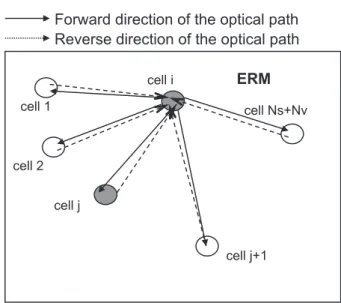
The "reciprocal Monte Carlo method" used in this thesis is also considered as one of the "reverse" techniques, it is firstly proposed by Taine (Taine et al. 2003) and then is validated by Tesse (2001).

The principle is that the optical path is considered in a reverse manner, which means a ray tracing can be used two times, both in the forward direction and in the reverse (reciprocal) direction as shown in Fig. 3.7. The power exchanged between a source cell (cell from which an optical path is built) and each cell crossed by the optical path is directly calculated. It

can be presented as4 _{(Tesse 2001):}

If a ray tracing can propagate from cell i to cell j, then it surely exists another ray tracing propagating from cell j to cell i following the same path. The ratio of the monochromatic energy emitted by cell i and absorbed by cell j to the monochromatic energy emitted by cell j and absorbed by cell i is equal to the ratio of the equilibrium spectral intensities of cell i and j Pea ν,ij Prea ν,ji = L 0 ν(Ti) L0 ν(Tj) (3.25) where Pea

ν,ij is the monochromatic energy emitted by cell i and absorbed by cell j in the

forward direction and Prea

ν,ji is the monochromatic energy emitted by cell j and absorbed by

cell i in the reciprocal direction using the same optical path. And their integrations in the frequency spectrum [0, +∞] are:

P_ijea=  ∞ 0 Pνea,ijdν (3.26) P_jirea=  ∞ 0 Pνrea,jidν (3.27) Cell i Cell j k_!,i k!,j !"#$%#&'&(#)*+",''-'.'/ i-0' 1)*(2#"*%3'&(#)*+",''-'.'/ j-(' P_ijea P_jirea

Figure 3.7 – Principe of the Reciprocal Monte Carlo Method

The rigorous demonstration of this principe provided by Tesse (2001) will be not repeated here, we juste make this principe to be understood by explaining the exchange formulation of radiative transfer presented in the Ph.D thesis of Tesse (2001). Considering an enclosure with non-isothermal opaque walls, containing a non-isothermal, heterogeneous, absorbing

and emitting medium. The medium and the walls are divided into Nv elementary volumes

4

Different authors have defined the reciprocal Monte Carlo method by different formulas. Here just the principe used in this thesis is presented.