HAL Id: tel-03208856
https://tel.archives-ouvertes.fr/tel-03208856
Submitted on 26 Apr 2021
HAL is a multi-disciplinary open access archive for the deposit and dissemination of sci-entific research documents, whether they are pub-lished or not. The documents may come from teaching and research institutions in France or
L’archive ouverte pluridisciplinaire HAL, est destinée au dépôt et à la diffusion de documents scientifiques de niveau recherche, publiés ou non, émanant des établissements d’enseignement et de recherche français ou étrangers, des laboratoires
Optimization of energy efficiency for residential
buildings by using artificial intelligence
Andrei Liviu Negrea
To cite this version:
Andrei Liviu Negrea. Optimization of energy efficiency for residential buildings by using artificial in-telligence. Architecture, space management. Université de Lyon; Universitatea politehnica (Bucarest), 2020. English. �NNT : 2020LYSEI090�. �tel-03208856�
N°d’ordre NNT : 2020LYSEI090
THESE de DOCTORAT DE L’UNIVERSITE DE LYON
Opérée au sein deINSA Lyon en cotutelle internationale avec
Université POLITEHNICA de Bucarest École Doctorale N° 162
Mécanique, Énergétique, Génie Civil, Acoustique (MEGA) Spécialité de doctorat : Thermique et Énergétique
Soutenue publiquement le 24/11/2020 par :
Negrea LIVIU ANDREI
Optimization of energy efficiency for residential
buildings by using artificial intelligence
Devant le jury composé de :
Professeur
Professeur
George DARIE (Université POLITEHNICA de Bucarest) Frank TILLENKAMP (ZHAW, Suisse)
Examinateur Rapporteur
Professeur Iolanda COLDA (UTCB, Roumanie) Rapporteur
Professeur Ion Hazyuk ( INSA Toulouse, France) Rapporteur Professeur
Professeur
Christian GHIAUS (INSA Lyon, France) Adrian BADEA (UPB, Roumanie
Co-directeur de thèse Directeur de thèse
Département FEDORA – INSA Lyon - Ecoles Doctorales – Quinquennal 2016-2020
SIGLE ÉCOLE DOCTORALE NOM ET COORDONNEES DU RESPONSABLE
CHIMIE CHIMIE DE LYON
http://www.edchimie-lyon.fr Sec. : Renée EL MELHEM Bât. Blaise PASCAL, 3e étage [email protected] INSA : R. GOURDON
M. Stéphane DANIELE
Institut de recherches sur la catalyse et l’environnement de Lyon IRCELYON-UMR 5256
Équipe CDFA
2 Avenue Albert EINSTEIN 69 626 Villeurbanne CEDEX [email protected] E.E.A. ÉLECTRONIQUE ÉLECTROTECHNIQUE AUTOMATIQUE http://edeea.ec-lyon.fr Sec. : M.C. HAVGOUDOUKIAN [email protected] M. Gérard SCORLETTI École Centrale de Lyon
36 Avenue Guy DE COLLONGUE 69 134 Écully
Tél : 04.72.18.60.97 Fax 04.78.43.37.17
E2M2 ÉVOLUTION, ÉCOSYSTÈME,
MICROBIOLOGIE, MODÉLISATION
http://e2m2.universite-lyon.fr Sec. : Sylvie ROBERJOT Bât. Atrium, UCB Lyon 1 Tél : 04.72.44.83.62 INSA : H. CHARLES
M. Fabrice CORDEY
CNRS UMR 5276 Lab. de géologie de Lyon Université Claude Bernard Lyon 1
Bât. Géode
2 Rue Raphaël DUBOIS 69 622 Villeurbanne CEDEX Tél : 06.07.53.89.13 [email protected] EDISS INTERDISCIPLINAIRE SCIENCES-SANTÉ http://www.ediss-lyon.fr Sec. : Sylvie ROBERJOT Bât. Atrium, UCB Lyon 1 Tél : 04.72.44.83.62 INSA : M. LAGARDE
Mme Emmanuelle CANET-SOULAS INSERM U1060, CarMeN lab, Univ. Lyon 1 Bâtiment IMBL
11 Avenue Jean CAPELLE INSA de Lyon 69 621 Villeurbanne Tél : 04.72.68.49.09 / Fax : 04.72.68.49.16 [email protected] INFOMATHS INFORMATIQUE ET METHÉMATIQUES http://edinfomaths.universite-lyon.fr Sec. : Renée EL MELHEM
Bât. Blaise PASCAL, 3e étage
Tél : 04.72.43.80.46 / Fax : 04.72.43.16.87 [email protected] M. Luca ZAMBONI Bât. Braconnier 43 Boulevard du 11 novembre 1918 69 622 Villeurbanne CEDEX Tél : 04.26.23.45.52 [email protected]
Matériaux MATÉRIAUX DE LYON
http://ed34.universite-lyon.fr Sec. : Marion COMBE
Tél : 04.72.43.71.70 / Fax : 04.72.43.87.12 Bât. Direction [email protected] M. Jean-Yves BUFFIÈRE INSA de Lyon MATEIS - Bât. Saint-Exupéry 7 Avenue Jean CAPELLE 69 621 Villeurbanne CEDEX
Tél : 04.72.43.71.70 / Fax : 04.72.43.85.28 [email protected]
MEGA MÉCANIQUE, ÉNERGÉTIQUE,
GÉNIE CIVIL, ACOUSTIQUE
http://edmega.universite-lyon.fr Sec. : Marion COMBE
Tél : 04.72.43.71.70 / Fax : 04.72.43.87.12 Bât. Direction [email protected] M. Philippe BOISSE INSA de Lyon Laboratoire LAMCOS Bâtiment Jacquard
25 bis Avenue Jean CAPELLE 69 621 Villeurbanne CEDEX
Tél : 04.72.43.71.70 / Fax : 04.72.43.72.37 [email protected]
ScSo ScSo*
http://ed483.univ-lyon2.fr Sec. : Viviane POLSINELLI Brigitte DUBOIS
INSA : J.Y. TOUSSAINT Tél : 04.78.69.72.76 [email protected] M. Christian MONTES Université Lyon 2 86 Rue Pasteur 69 365 Lyon CEDEX 07 [email protected]
“Success is not final; failure is not fatal:
It is the courage to continue that counts.”
Winston S. Churchill
Acknowledgements
“If you really look closely, most overnight successes took a long time.” – Steve Jobs
To be honest, words cannot describe the passion, dedication, and attitude this doctoral thesis managed to invoke within my personality, and I could have never done it without the people I appreciate the most. Few moments after the defense of my dissertation, four out of five professors granted me the opportunity to follow a PhD in energy field and, by accepting it, has been the most beautiful period in my entire life. This life-changing experience made me realize the importance of failure, which is not fatal, and that courage to pursue towards my goal is the only thing that matters. By all means I would like to express my appreciation to the persons that believed in me until the end of this chapter.
Firstly, I would like to set up how this PhD thesis was carried out. Gratitude for Doctoral School of the Faculty of Power Engineering within University POLITEHNICA of Bucharest and Centre for Energy and Thermal Sciences of Lyon (CETHIL) under the
guidance of Prof. Dr. Ing. Adrian Badea and Professor Jocelyn Bonjour. Also, many thanks to GDF SUEZ and Erasmus Plus for financing me during this amazing exchange I had in Lyon, France.
I would like to begin with the person that had an eagle-eye for my aptitudes and dedication. I am deeply grateful to my supervisor Professor Adrian Badea who made this possible and gave me the opportunity to widen my environment and finish this thesis. Within his ongoing assistance, Professor Adrian Badea believed in me, even if tough challenges were encountered.
I would like to state my deepest appreciation to my mentor from CETHIL Professor Christian Ghiaus for the continuous support of my PhD thesis, for his patience, motivation, and tremendous knowledge. His guidance and persuasion helped me throughout time of research and writing of this thesis. I could not have imagined having a better advisor and mentor for my PhD study without whom this could have not been possible.
I would like also to extend my innermost gratitude to Professor Vladimir Tanasiev for every opportunity he gave me, for every mistake that he pointed out, for every late night hour that he would have emailed me and, of course, for every moment that he believed in my aptitudes. All the research studies that I wrote are the proof that Vladimir Tanasiev gave me motivation, courage, and appreciation of what I could gain in knowledge.
Besides my advisor, I would like to thank the rest of my thesis committee: Prof. Horia Necula, Prof. Cristian Dinca and Prof. George Darie, for their insightful comments and encouragement, but also for the hard question they bring into equation which widen my research from various perspectives point of view.
My sincere thanks also go to Prof. Horia Necula for asking me all the time about the status of my thesis and when shall I present it. Moreover, I would like to extend my sincere thanks to Prof. George Darie for keeping my enthusiasm high enough to finish this doctoral
thesis, for his valuable advices, and for leading me into selecting the best option for my career.
I’d like to acknowledge the assistance received though cooperative work conducted in CETHIL laboratory and to the summer School in 2016 organized by DYNASTEE-INIVE and CITIES and Civil Engineering School (university of Granada, Spain) in collaboration with CIEMAT (Spain), DTU (Lyngby, Denmark) and ESRU (Strathclyde University, Glasgow) who made me realized the importance of homework and deadlines.
I thank to my fellow Romanian doctoral and post-doctoral lab-mates for the amazing working atmosphere we had, for encouraging me, for stimulating my working desire, for the sleepless nights working together before research deadlines and for the fun we had during these years. Also, special thanks to Diana Robescu for working with me and encouraging my efforts. I especially thank Professor Diana Cocarta for sharing her experience during this period and encouraging me to succeed.
Sincere appreciation to Professor Cristian Dinca for all the support, invaluable contribution, practical suggestion, and constructive criticism which all lead to my success.
Last but not the least, I would like to say couple of words to my family, and friends. To all my friends that stood beside me and asked me every time they see me: “Will
you ever finish your thesis?” I express my gratitude and say thanks for the support during all
the difficult moments I have had. Your kind words pushed me further in concluding this chapter.
Mother, I know it has been a long road but I would like to sincerely appreciate your support and not giving up on me, even if I was stubborn and didn’t want to talk about my thesis status. Your advices, life experience, patience that cannot be underestimated, made me grow and persuade this PhD thesis.
“Father, I made it!” – PhD Liviu Andrei Negrea
I would dedicate this manuscript to my father, Negrea Gheorghe, which has a forever place in my heart, telling you that I know that from up there, you have been supporting, guiding, advising, trusting, helping, and showing me that the secret of success is by taking small steps one at a time.
Abstract
Consumption, in general, represents the process of using a type of resource where savings needs to be done. Energy consumption has become one the main issue of urbanization and energy crisis as the fossil depletion and global warming put under threat the planet energy utilization.
In this thesis, an automatic control of energy was developed to reduce energy
consumption in residential area and passive house buildings. A mathematical model founded on empirical measurements was developed to emphasize the behavior of a testing laboratory from UPB. The experimental protocol was carried out following actions such as: building parameters database, collecting weather data, intake of auxiliary flows while considering the controlling factors. The control algorithm is controlling the system which can maintain a comfortable temperature within the building with minimum energy consumption.
Measurements and data acquisition have been setup on two different levels: weather and buildings data. The data collection is gathered on a server which was implemented into the testing facility running a complex algorithm which can control energy consumption. The thesis reports several numerical methods for estimating the energy consumption that is further used with the control algorithm.
An experimental showcase based on dynamic calculation methods for building energy performance assessments was made in Granada, Spain, information which was later used in this thesis. Estimation of model parameters (resistances and capacities) with prediction of heat flow was made using nodal method, based on physical elements, input data and weather information. Prediction of energy consumption using state-space modeling show improved results while IoT data collection was uploaded on a Raspberry Pi system.
All these results were stable showing impressive progress in the prediction of energy consumption and their application in energy field.
Keywords: energy prediction, energy consumption, IoT, control algorithm, human behavior
Résumé
La consommation, en général, représente le processus d’utilisation d’un type de ressource où des économies doivent être réalisées. La consommation d’énergie est devenue l’un des principaux problèmes d’urbanisation et de crise énergétique, car l’épuisement des combustibles fossiles et le réchauffement climatique mettent en péril l’utilisation de l’énergie des plantes. Cette thèse présent une méthode d’économie d’énergie a été adoptée pour la réduction de consommation d’énergie prévu le secteur résidentiel et les maisons passives. Un modèle mathématique basé sur des mesures expérimentales a été développé pour simuler le comportement d’un laboratoire d’essai de l’UPB. Le protocole expérimental a été réalisé à la suite d’actions telles que : la construction de bases de données sur les paramètres, la collecte de données météorologiques, l’apport de flux auxiliaires tout en considérant le comportement humain.
L’algorithme de contrôle-commande du système est capable de maintenir une température constante à l’intérieur du bâtiment avec une consommation minimale d’énergie. Les mesures et l’acquisition de données ont été configurées à deux niveaux différents : les données météorologiques et les données sur les bâtiments. La collection de données est faite sur un serveur qui a été mis en œuvre dans l’installation de test en cours d’exécution d’un algorithme complexe qui peut fournir le contrôle de consommation d’énergie.
La thèse rapporte plusieurs méthodes numériques pour envisage la consommation d’énergie, utilisée avec l’algorithme de contrôle. Un cas expérimental basé sur des méthodes de calcul dynamiques pour les évaluations de performance énergétique de construction a été faite à Grenade, en Espagne, l’information qui a été plus tard utilisée dans cette thèse.
L’estimation des paramètres R-C avec la prévision du flux de chaleur a été faite en utilisant la méthode nodal, basée sur des éléments physiques, des données d’entrée et des informations météorologiques. La prévision d’énergie de consommation présent des résultats améliorés tandis que la collecte de données IoT a été téléchargée sur une carte à base de système de tarte aux framboises. Tous ces résultats ont été stables montrant des progrès impressionnants dans la prévision de la consommation d’énergie et leur application en énergie.
Mots-clés : prévision énergétique, consommation d’énergie, IoT, algorithme de contrôle, comportement humain
Nomenclature
Notational conventions
𝑥, 𝑦, 𝑧 Scalars
𝐱, 𝐲, 𝐳 Vectors
𝐀, 𝐁, 𝐂 Matrices or fuzzy inputs, set of rules
R Fuzzy output, by composing fuzzy inputs and set of rules
ℝ𝑞 Space of dimension 𝑞 Notations 𝐀T Matrix transpose 𝐀−1 Matrix inverse 𝐀−𝟏/𝟐 (𝐀1/2)−1 𝐀−T/𝟐 (𝐀−1/2)T
det(𝐀) Determinant of the matrix 𝐀 tr(𝐀) Trace of the matrix 𝐀
𝐱̇ Time derivative of the vector 𝐱
𝜕𝐱 𝜕𝜃⁄ 𝑖 Partial derivative of 𝐱 with respect to 𝜃𝑖
𝐝𝐢𝐚𝐠(𝑎1, 𝑎2, … , 𝑎𝑁) Diagonal matrix with diagonal values 𝑎1, 𝑎2, … , 𝑎𝑁 𝔼(𝐱) Expected value of a random variable 𝐱
𝕍(𝐱) Variance of a random variable 𝐱
𝕍(𝐱, 𝐲) Covariance between the random variables 𝐱 and 𝐲 𝑝(𝐱) Probability density function (pdf) of a random variable 𝐱 𝑝(𝐱|𝐲) Conditional pdf of the vector 𝐱 given the vector 𝐲
𝐱 ~ 𝑝(𝐱) Random variable 𝐱 with probability distribution 𝑝(𝐱) 𝒩(𝐦, 𝐏) Gaussian pdf with mean vector 𝐦 and covariance matrix 𝐏 𝒢(𝑎, 𝑏) Gamma distribution with shape 𝑎 and expected value 𝑏 𝛽(𝑎, 𝑏, 𝜃min, 𝜃max) Beta distribution with shape parameters 𝑎 and 𝑏, lower bound
𝜃min and upper bound 𝜃max
𝒰(𝜃min, 𝜃max) Uniform distribution between the lower bound 𝜃min and upper
bound 𝜃max
∝ Proportional
≈ Approximately equal
𝐱1:𝑁 Set of values 𝐱 = [𝐱1, 𝐱2, … , 𝐱𝑁] 𝑭(𝐱) Function of the states x
Q Reactive power V Voltage I Current F Frequency 𝑘 Boltzmann constant Ω Quantum-mechanically ℎ Convection coefficient S Surface
0 black body radiation coefficient
T Temperature
𝜆 Thermal conductivity
𝑄, 𝑞𝑠 Heat flux and heat surface flux 𝜂ℎ Efficiency of the heating system
𝐶0 Thermal capacity
𝑓0 Heat rate source
G Diagonal matrix of conductance of size adequate to the number of rows of A
C Diagonal matrix of capacitances of dimension equal to the number of columns of A
b Vector of temperature sources location of dimension adequate to the number of rows of A
f Vector of flow sources location of dimension equal to the number of columns of A
y Vector of temperature outputs of dimension size A,2 𝑞𝑖(𝑡) Heat flow rate density – interior
𝑞𝑒(𝑡) Heat flow rate density – exterior
θ𝑖(𝑡) Indoor values
θ𝑒(𝑡) Outdoor values
R Thermal resistance
𝐶𝑖 Interior thermal capacity
Abbreviations
A.I. Artificial intelligence
ASHRAE American society of heating, refrigerating, and air-conditioning ANN Artificial neural networks
ARMAX Autoregressive moving average model BMS Building energy management system
CDD Cooling Degree day
CTMS Continuous time stochastic modelling CRUD Create, read, update and delete data CMS Content management system CSV Comma separated value
COSEM Companion Specification for Energy Metering
DD Degree day (K day)
DHW Domestic Hot Water
EAHX Earth to air heat exchanger
EF Entity Framework
EU European Union
FIRM Impulse response models
F Free force
HTTP Hypertext transfer protocol
HVAC Heating, ventilation, and air conditioning HMI Human machine interface
HDD Heating degree day
HED Heating demand (kWh) IHG Internal Heat Gain
IHD In home display
IoT Internet of things
LQR Linear quadratic regulator
MQTT Message queuing telemetry transport MVHR Mechanical ventilation with heat recovery nZeb Nearly zero energy building
OHL Overall heat loss coefficient (kW K−1)
OS Operation System
PID Proportional-integral-derivative PI Proportional integral
Pa Pascals
PD Proportional derivative
SMX Smart meter extension
S Entropy
SOAP Simple object access protocol SOA Service oriented architecture SBC Smart Building Controller SQL Programming language
SD Secure Digital
TFA Treat Floor Area
TZ Trusted zone
T Temperature
UPB University POLITEHNICA of Bucharest VPN Virtual private network
WSN Wireless sensor network
WAN Wide area network
WWW World wide web
Contents
Acknowledgements ... 6 Abstract ... 8 Résumé ... 9 Nomenclature ... 10 Abbreviations ... 12 Contents ... 14 List of figures... 17 List of tables ... 20CHAPTER I – Global general introduction ... 21
State of the problem ... 22
Outline of the thesis ... 25
General presentation of control algorithms ... 29
1.3.1. Classic – PID... 30
1.3.2. Modern control: state-space and optimization ... 32
1.3.3. Intelligent control: fuzzy and artificial neuronal networks ... 34
CHAPTER II – Testing facility ... 41
Introduction ... 42
2.1.1. Heating ventilating and air conditioning ... 43
2.1.2. PV panels ... 43
2.1.3. Off grid system ... 43
2.1.4. Smart solution system ... 44
Passive house concept... 44
Passive house requirements ... 45
Physical characteristics ... 47
Heating, ventilation, and air conditioning system ... 51
Monitoring system ... 53
2.6.1. Software ... 53
2.6.2. Data storage and database ... 56
2.6.3. Communication ... 58
Conclusions ... 61
CHAPTER III – Measurements and data acquisition ... 62
Introduction ... 63
SMX (smart meter extension) ... 65
Starting the SMX application ... 67
Description of SMXCores ... 72
Starting SMXCore modules ... 74
3.5.1. MeterVirtual - Module ... 75
3.5.2. Physical meter module ... 75
3.5.3. Database module ... 76
3.5.4. MQTTClient - Module ... 76
3.5.5. Storage module ... 77
3.5.6. MeterDLMS client modules ... 77
Physical and electrical input parameters acquisition ... 79
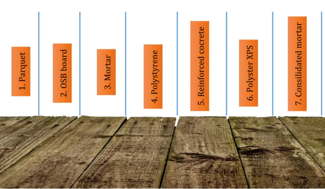
3.6.1. Data collection and experimental wall details ... 79
3.6.2. Types of data ... 81
3.6.3. Classification of data and acquisition ... 82
Data collection and integration through IoT ... 85
Statistical analysis of weather prediction ... 89
3.8.1. Weather data acquisition ... 91
3.8.2. Weather input algorithm ... 95
Example results ... 97
3.9.1. Physical and electrical acquisition ... 97
3.9.2. Results and interpretation of IoT ...101
Conclusion ...105
CHAPTER IV – Energy prediction based on small amount of information: degree-day and grey-box models ... 106
Degree-day method ...107
4.1.1. Base temperature (balance point) ...109
4.1.2. Heating/cooling and degree-day calculation ...110
Grey-box models ...115
4.2.1. Introduction ...115
4.2.2. Grey-box identification model...116
4.2.3. Conclusion ...122
CHAPTER V – Energy monitoring and control ... 124
Introduction ...125
Thermal comfort in buildings using fuzzy logic ...125
Fuzzy algorithm ...129
Results and interpretation ...132
Conclusion ...134
CHAPTER VI – Conclusions and perspectives ... 135
Introduction ...136
Thesis goal ...136
Thesis contribution ...137 5.4
Thesis outlook ...138
Appendices ... 139
Testing facility ...139
In_Situ_Wall MATLAB code ...142
Policy exemplification code ...144
Content of Modules from Chapter III ...146
7.4.1. Modules.txt ...146
7.4.2. MeterVirtual - modules ...146
7.4.3. Meter IEC6205621 - Module ...147
7.4.4. Mongo database client – module ...148
7.4.5. MQTTClient - Modules ...150
7.4.6. File Storage - Module ...151
7.4.7. Metere DLMS Client - module ...152
Weather data algorithm and implementation ...154
List of figures
Fig. 1-1 Global primary energy utilization [5] ... 23
Fig. 1-2 Statistical share of energy from renewable sources in EU member states [10] ... 24
Fig. 1-3 Example of student campus [20] and residential district [21] ... 26
Fig. 1-4 Model for system inputs and outputs ... 26
Fig. 1-5 Diagram for mathematical model in-use ... 27
Fig. 1-6 Example of mathematical model for a specific physical part of the house ... 27
Fig. 1-7 Simple comparison between examination types [22] ... 27
Fig. 1-8 Fast comparison between examination types [22][26] ... 28
Fig. 1-9 General representation of a system ... 30
Fig. 1-10 PID controller with feedback ... 31
Fig. 1-11 PID controller with feedback and integrator ... 31
Fig. 1-12 PID controller with feedback, proportiona; integral and derivative actions ... 32
Fig. 1-13 Bloc diagram of control fuzzy algorithm ... 35
Fig. 1-14 Artificial neural network architecture [77] ... 38
Fig. 1-15 Comparison between artificial intelligence (AI) algorithms [78] ... 39
Fig. 2-1 UPB Pasive House ... 42
Fig. 2-2 Basic principles of a Passive House [83] ... 45
Fig. 2-3 Rooftop elements of the Passive House UPB ... 47
Fig. 2-4 Exterior walls of the Passive House UPB ... 48
Fig. 2-5 Triple glazed windows of the Passive House UPB ... 48
Fig. 2-6 Floor slab of the building ... 49
Fig. 2-7 Partition wall of the passive House UPB... 50
Fig. 2-8 Exterior Door of the passive House UPB ... 51
Fig. 2-9 The HVAC system of eastern house (EAHX) [89] ... 52
Fig. 2-10 The HVAC system of western house [85] ... 53
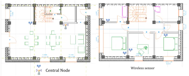
Fig. 2-11 The placement of wired sensors in the HVAC system [90] ... 54
Fig. 2-12 Monitoring system structure [91] ... 55
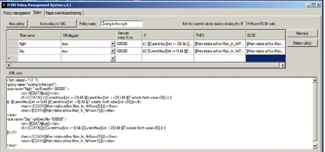
Fig. 2-13 Policy Management System – FCINT ... 56
Fig. 2-14 Visual Studio software - data mapping system of UPB passive house [93] ... 57
Fig. 2-15 WiFi sensor ... 59
Fig. 2-16 Distribution of the wired and wireless sensors ... 60
Fig. 3-1 Forward and data-driven approach ... 64
Fig. 3-2 Basic architecture of Smart Meter eXtension modules ... 66
Fig. 3-3 Configuration of a MQTT broker ... 68
Fig. 3-4 MQTT Lens visualization of the voltage on phase 1 ... 69
Fig. 3-5 MQTT Lens visualization of the 3 different measurements U, P1, and A+ ... 70
Fig. 3-6 SMX-HMI example ... 72
Fig. 3-7 SMXCore modules (current situation, other modules may appear) ... 73
Fig. 3-8 Example of SMXCore modules instantiation ... 74
Fig. 3-9 Trace file message analysis ... 78
Fig. 3-11 Communication protocols [99] ... 82
Fig. 3-12 SMX architecture [99] ... 83
Fig. 3-13 Connectivity and zones [99] ... 83
Fig. 3-14 Data workflow [99] ... 84
Fig. 3-15 Three dimensional states of the IoT model ... 86
Fig. 3-16 Data exchange information prototype [109] ... 87
Fig. 3-17 Functionality of a Sparrow node block diagram ... 88
Fig. 3-18 Weather parameters ... 90
Fig. 3-19 Hourly weather parameters ... 92
Fig. 3-20 Weather data prediction for 4 days ahead ... 93
Fig. 3-21 Prediction input data from WeForecast ... 93
Fig. 3-22 Wunderground prediction data ... 94
Fig. 3-23 Wunderground calendar - forecast for 30 days in advance ... 94
Fig. 3-24 EPW file downloaded from Energy Plus website [114] ... 95
Fig. 3-25 Energy Plus CSV file [113] ... 96
Fig. 3-26 Voltage evolution [99] ... 98
Fig. 3-27 Current evolution on a 24h day log [99] ... 99
Fig. 3-28 Power factor variation [99] ... 100
Fig. 3-29 PV Production [99] ... 100
Fig. 3-30 IoT tools [109] ... 101
Fig. 3-31 S1 and S2 as dust sensors [109]... 101
Fig. 3-32 Dust sensor S1 - data acquisition [109] ... 102
Fig. 3-33 The evolution of parameter gathered on 22th of August [109] ... 102
Fig. 3-34 Sensor comfort parameters [109] ... 102
Fig. 3-35 Temperature evolution on a selected day of August [109] ... 103
Fig. 3-36 Data about comfort parameters [109] ... 103
Fig. 3-37 Edge platform ... 104
Fig. 4-1 Trend in heating and cooling – EU members [119] ... 107
Fig. 4-2 Theoretical relationship between temperature and energy use [122] ... 110
Fig. 4-3 Energy balance of the testing laboratory ... 112
Fig. 4-4 Specific losses, gains, heating demand (kWh/m2 month - Reference to habitable area) ... 113
Fig. 4-5 Monthly specific heat demand calculation ... 114
Fig. 4-6 Specific losses, loads and cooling demand (kWh/m2 month) ... 114
Fig. 4-7 Monthly cooling request calculation ... 115
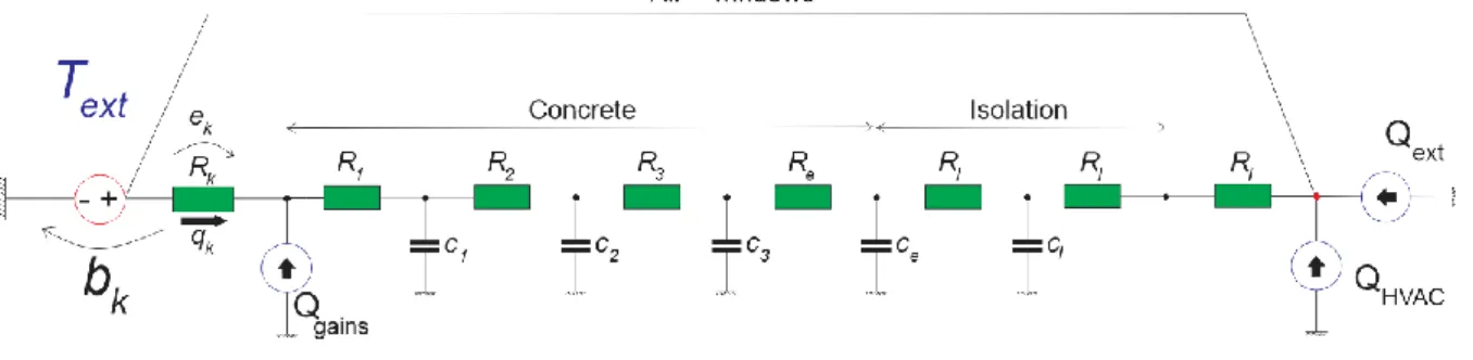
Fig. 4-8 RC diagram ... 116
Fig. 4-9 Residuals, inputs and outputs of the system ... 117
Fig. 4-10 The correlation of residuals and white noise ... 117
Fig. 4-11 Nodal form with solar radiation ... 118
Fig. 4-12 The system with solar radiation implementation ... 119
Fig. 4-13 Mathematical model with solar radiation and steady point ... 120
Fig. 4-17 Residuals and results ... 122
Fig. 5-1 Fuzzy mechanism ... 126
Fig. 5-2 Specific example of using ANN with fuzzy logic ... 127
Fig. 5-3 Structure of fuzzy implementation ... 127
Fig. 5-4 Fuzzy system appliance ... 128
Fig. 5-5 Membership level of fuzzy logic algorithm ... 128
Fig. 5-6 Fuzzy membership functions ... 129
Fig. 5-7 Implementation of fuzzy rules ... 130
Fig. 5-8 Fuzzy logic testing system ... 131
Fig. 5-9 Policy line code ... 132
Fig. 5-10 Variation of heating and ventilation energy consumption [90] ... 132
Fig. 5-11 Evolution of indoor and outdoor temperature ... 133
Fig. 5-12 Temperatures variation between N and South [109] ... 133
Fig. 7-1 Ground floor of the testing facilty ... 139
Fig. 7-2 Ground floor elements ... 140
Fig. 7-3 1st floor of the testing facility ... 141
List of tables
Table 1-1 Potential of distinct forward and data-driven algorithms ... 40
Table 2-1. Geometrical aspect of the UPB Passive House ... 42
Table 2-2. Thermal characteristic of the UPB Passive House [85] ... 46
Table 2-3 Main properties of window triple glazed windows ... 49
Table 2-4 U-values of the buildings elements foor slab ... 50
Table 2-5 Server data storage table ... 57
Table 2-6 UPB WiFi sensor ... 59
Table 3-1 Data_Series1 example ... 80
Table 3-2 Data_Series 2 example ... 80
Table 3-3. IoT ecosystem – important elements [109] ... 86
Table 3-4 Inside and Outside temperature variation ... 90
CHAPTER I – Global general introduction
The purpose of this chapter is to present the problem of world’s energy
consumption, especially in urban area. This thesis responds to nowadays concerns and to the necessity to decrease the energy consumption in buildings.
The potential reduction in energy consumption in Romania shows increased potential as the statistics from EU display. The thesis outline is covered in the upcoming section, along with the control algorithms presentation.
This part gives attention to relevant data, suitable to the achievement provided in this essay.
State of the problem
The world’s energy consumption problem has become one of the most appealing subjects in 2020 because of the progress in urbanization and advancement of networking society [1]. The planet is under serious threat due to energy crisis because of fossil energy depletion and global warming determined by harmful gases. Therefore, ideas and projects on “how to save energy”, are among the most common subjects on every social debate. New ways of producing energy must be found in order to combat energy crisis.
To be more specific, energy needs to be conserved, saved and produced by other means than the actual ones [2]. In order to understand the energy laws, facts about thermodynamics need to be considered. To put it differently, energy may seem to be the problem but, from a thermodynamic point of view, the increase in entropy is the problem. In physics, energy stands for the ability of moving an object from a location X to a location Y. Location can be take into consideration as point.
Therefore, it exists two large types of mechanical energy:
1) Kinetic energy (responsible for moving an object to one-half of its specific mass and the square of its velocity)
2) Potential energy (responsible for storing energy by multiplying mass, gravitational energy and height or location)
Energy can be transformed from one form to another while creating an additional type: thermodynamic energy. When an object is moving from its location to another with a specific velocity, kinetic energy is evacuated progressively, creating heating, representing the 1st law
of thermodynamics: “In any isolated system, total energy is preserved”[3]. To put it in another illustration, there are different forms of energy: 1) useful (stand for kinetic, potential, chemical energy, electricity etc.). 2) useless (thermodynamic energy).
To clarify, we might think useful energy as a specific free-force (𝐹) applied to an object while useless energy is the multiplication of temperature (𝑇) by entropy (𝑆)
demonstrating the 2nd law of thermodynamics: “Entropy is rising in any isolated system” [3]. Additionally, entropy can measure the energy quality inside any object.
All things considered, from a physics perspective point of view, the energy crisis is an entropy crisis due to its property of increasing in any closed system.
The subject proposed in this thesis responds to nowadays concerns and to the necessity to decrease the generated power consumption in buildings, especially in the residential sector. A data report regarding energy efficiency in buildings, realized by ENERGDATA in 2014, shows that the energy price grew with 64 % from 2004 to present. The energy costs of residential sector reached a peak of 40 % consumption for the entire Europe, while in Romania the prices were close to 44.4 % of the electricity price tag [4].
Taking into account the planet’s renewable resources, the energy consumption relies on several factors: hydro, nuclear, natural gas, coal, geothermal, wind, solar and, the biggest, oil. In 2017, the global primary energy consumption is divided as shown in Fig. 1-1.
Fig. 1-1 Global primary energy utilization [5]
Due to a strategic energy action plan approved by Romania for 2007-2020 period, a potential reduction in energy consumption was identified for the residential sector. After a statistical analysis, the potential of energy reduction in Romania is estimated, depending on the sector they belong, to 30 – 50 % for residential and 13 – 19 % for tertiary sector. The consumption for space heating in buildings in Europe represents 67 % of the total energy consumed in buildings (Romania has a total consumption of 50 %), dragging attention to the potential energy savings that can be done.
Guidelines of energy savings and energy production from renewable in Romania are set up at 38 % until 2020 [6]. Romania has a potential of 43.2 % of electricity generation using technologies that involve renewable energy sources. The new strategic plan for the upcoming years is aiming to cut 20 % of energy production which is harmful for the
environment. For example, 20 % cutoff from residential green-house effect gas emissions is a must until 2020. On the other hand, 20 % more energy production from unconventional sources is listed as a future priority. At the same time, smart technologies come in support from the Romanian’s energy potential proving that real time data collection, small monitoring devices or data awareness administration can increase the energy efficiency by up to 20 % [7]–[9].
Due to the high potential of energy savings, EU’s reports regarding the national targets in sharing renewable energy sources declared Romania as completing her task before the deadline. Bulgaria, Croatia and Montenegro managed to reach their targets as well, while Luxembourg and Malta are on track for reaching this goal. In Fig. 1-2, a detailed explanation regarding the gross in final energy consumption is presented, according to Eurostat.
Fig. 1-2 Statistical share of energy from renewable sources in EU member states [10] The ability of mankind to satisfy the demands of the today’s generation without concession the capacity of forthcoming generation to face its own demands is defined as sustainable development [11]. The global economy has to accelerate its growth in order to improve the lifestyle and therefore the progress. The energy consumption rate is one of the major threats that EU member states are confronting, trying to develop methods to improve the energy savings. For a detailed list of global energy data, International Energy Agency is sharing useful information on their website [12].
This thesis focuses on the usage of artificial intelligence to optimize the energy
performances of residential buildings, emphasizing a huge impact on sustainable development from two standpoints.
The first angle is the energy management optimization for residential buildings, representing an increase in energy efficiency that leads to sustainable development and draining renewable energy from unlimited sources.
The second angle is the integration of clean technologies through the usage of artificial intelligence to increase the energy performances in buildings. The adoption of this type of technology reduces the incidence of industrial leftovers on the environment by preventing pollution and by savings money [13]. In general, through energy efficiency we obtain:
- reduction in usage of raw materials, - reduction in pollutant emission, - reduction in waste,
- improved air quality - improved living conditions
Therefore, the prediction of energy demand for heating and cooling loads, presents the main factors in identifying measures to lower energy consumption. The thesis aims to develop a set of services that allows modeling, verification, and control of equipment of testing
laboratory. In order to create specific conditions of thermal comfort, certain methods can be applied. These methods imply having as inputs a set of measured parameters (indoor
temperature, outdoor temperature, energy consumption, solar radiation, humidity or generated energy from renewable energy sources, energy flux) and a set of building characteristics (construction material) to provide an energy prediction with low errors to lower the utilization of energy in buildings.
Residential, educational institutes and office buildings are accountable for the high energy consumption within community energy usage. Considerable amount of energy
consumption should be utilized to supply energy systems in order to provide thermal comfort [14]. Moreover, when trying to discover a specific energy benchmark for residential buildings inside and outside circumstances should be taken into consideration [15], [16].
It is important to notice that thermal comfort has always been the highest consumer when talking about human needs. “A state in which there are no driving impulses to correct
the environment by the behavior” is the characterization of thermal comfort as Hensen
explained [17]. To complete the sentence, ASHRAE outlined this phenomenon as “the
condition of mind in which satisfaction is expressed with the thermal environment” [18].
Based on the above interpretations, thermal comfort could be identified as a state of mind, body, cognitive process, and not referring to a state of condition. Among people, thermal perception may differ radically, even if they are situated in the same environment. A more reliable explanation about thermal comfort methods, physiological comfort, mathematical modeling on energy transfer between human organism and surroundings can be found on N. Djongyang paper [19].
The thesis focuses on three modes of operation for the building:
1. Passive operation, which takes into account thermal conditions using passive sources (operation of window, shutters and doors etc.).
2. Hybrid operation, which implies the simultaneous use of passive installations and active HVAC systems.
3. Mechanical operation, which consists in ensuring thermal comfort by using only the HVAC facilities available in the building.
Outline of the thesis
Firstly, a mathematical model that is based on experimental measurements to simulate the behavior of the building was developed. The system was implemented on a passive house from UPB, with a development perspective to a student campus or to a residential district, as figured in Fig. 1-3.
Fig. 1-3 Example of student campus [20] and residential district [21] The experimental protocol was implemented by following these steps: - Build the input parameter’s database - indicating the system sensors.
- Collect weather data (solar intake, wind, humidity, cloud coverage) – for example, solar intake performs an important aspect for the laboratory, as external parameters influence the thermal comportment of the house.
- Intake of auxiliary flows (the flow injected by the HVAC system - Control the house temperature.
Fig. 1-4 Model for system inputs and outputs
The model for the system inputs and outputs, as presented in Fig. 1-4, is consists of three significant areas. The first part, indicated by the left side, contains information about input data of the system such as weather data and auxiliary heat flow rates. The middle part represents a mathematical model able to process the input data and to predict the future input data in order to respond with a precise output. The model is responsible for the connection between inputs and outputs. The right side is the output calculation that has double role. The output is used for:
- Harvest the necessary variables for the system (such as interior temperature or energy consumption).
Fig. 1-5 Diagram for mathematical model in-use
A closer sample of system model for entries and outputs is exemplified in Fig. 1-5 with the implementation of a control system into the model. The HVAC heat flow rate is computed as a new input for the mathematical model to control inside temperature. Another modification to the system is the implementation of set-point temperature, as a control system for the mathematical model to receive a new input. In Fig. 1-6, a particular example of such a model is presented. The exterior heat flow is passing through the wall of the house changing into an interior temperature and outputting the flux of the system.
Fig. 1-6 Example of mathematical model for a specific physical part of the house
To obtain the numerical model, a full analysis of a physical phenomenon of the house is required. To solve and analyze the mathematical model, we can use several models (Fig. 1-7):
• white box – full knowledge about the implemented system, • black box – zero knowledge about the implemented system,
• grey box – some knowledge about the implemented system, physical and statistical. A white box model handles the thermal modeling of the building for solving the heat transfer equations. This method type is very laborious, requiring a large amount of data about the analyzed house. White box is perfectly applied in the context where there are many
physical data about the building (material properties, geometry of the building, characteristics, localization, heating and cooling system). The white box type is based on nodal approaches, reviewing the functioning of the applications rather than its functionalities [23].
A black box model handles the correlation between output and input data. This correlation may give good results, but it is not scientifically justified. Within the black box, the system requires huge amount of historical data as input, while requesting none for physical interpretation [24], [25].
Fig. 1-8 Fast comparison between examination types [22][26]
A grey box model is a hybrid method that can help solving a system in a fast manner, because it is capable to simulate the house’s thermal behavior and to optimize the input
house is realized, when it is incomplete or does not provide enough details about the system. In Fig. 1-8 a fast comparison underlining the most important properties of each testing model.
Artificial neural networks (ANN) are frequently used in artificial intelligence (A.I.) applied on human behavior prediction application [27]. Artificial neural networks will be used to build nonlinear systems as they have the ability to adapt to specific operating mode of the building. Special attention will be given to the artificial neural network comportment during the heating/cooling of the building [28]–[30].
As a conclusion, it is fundamental to acknowledge the energy consumption of the house due to the following perspectives [31]:
- Estimation and parameters calculation of a building (sizing of thermal installation and cooling systems).
- Calculation of consumer costs. - Optimization for reduction of costs.
Therefore, the cost forecast, starting from energy loads for heating and cooling, is important for identifying the parameters that can decrease energy consumption. Some fields of applicability are:
- Financial planning: it is important to know the costs for a month in advance. For example, the users can plan their own financial resources.
- House behavior: artificial intelligence can be used for predictive control. For example, the solar radiation can be estimated so that, if the inside temperature indicates 20 °C and the outside temperature indicates 15 °C, to decide that it’s useless the usage of heating.
- Planning of exhaustible sources: if we analyze from another perspective, human behavior impacts directly the house in study. We can build scenarios in accordance with heating/cooling timetables, depending on each user behavior. As an example, we can imagine a network of residential buildings. If it is forecasted that in October the fuel reserves will end, then we can make a planning of the financial resources and we can provide fuel in a timely manner.
General presentation of control algorithms
Buildings efficiency is stated as energy by unit of surface, kWh/m2 [32], even if EU regulation began to use carbon dioxide production (kg CO2/m2year) [33]. Regardless the fact
that the building temperature can be controlled by classical control algorithms [34], intelligent energy management can learn the behavior of the building [35].
Taken into account buildings control strategies and experience, multiple domestic and outdoor disturbances have been claimed to affect the thermal behavior of any system. Thus, the main task of a controller is to adjust thermal conditions [36]. Moreover, as reported by Wong [37], specific criteria should be implemented in the interest of obtaining the desire thermal comfort depending on human knowledge or judgement.
- field,
- management, - control.
In order to be fully efficient, when creating an algorithm, it is required to break the overall procedure in smaller control-command systems. For this, Salsbury separated HVAC control in central units, air pieces and terminal devices [38]. The central units are responsible for generating heating and cooling of the inside temperature using PID (proportional-integral-derivative) controller. The PID will be detailed in the upcoming sub-chapter emphasizing the response of the system with few modifications. Part of the field level control are the empirical model suitable to support dynamic prototype analysis [39]. Secondary control management level refers to all scenes of building’s functionality demands like BMS (building energy management). As the system becomes flexible and complex, every buildings component can be automatically controlled [40]. With this in mind, human comfort is presented as the most significant constituent due to the rate of change [41].
1.3.1. Classic – PID
A PID controller is composed of: - P, proportional controller,
- I, integrator and, - D, differential action.
The proportional part adjusts the error through multiplication of the deviation between the set-point and the measurement with a constant. The Integrator (I) corrects the control signal by integrating the error in time. By including the integral to the systems activity, it dispels the offset but decreases the system stability. In order to combat this situation, the Differential (D) operations further introduced, rectifies the low frequency flaws collected by the Integrator. The benefit of using the Differential action is due to its ability to quickly modify errors values, disregarding the delayed values. For the purpose of getting optimal and accurate results out of a PID control, specific configuration and constant setup must be taken into account. Several auto-tuning [42], open loop steps [43] have been taken as a response, a solution for this issue, as well as adaptive algorithms [44].
The PID interacts with system that is controlled. The system has input and output variables. Inputs are presented as the actual signal delivered to the ecosystem as long as output result are the controlled variables. The basic idea of the control system is to understand how to generate the input signal in order for the system to produce the required variable – meaning the output, as shown in Fig. 1-9:
In order to achieve the desired behavior of the system, a set-point variable, or the required values, need to be taken as reference. Additionally, the output of the system is feedbacked and compared with the set-point to assess how far off the system is from where we wanted to be. As displayed in Fig. 1-10, the difference between the feedback and the commanded variable is known as the error term. The goal of the system is to achieve zero error. This is possible by implementing a PID controller. In this regard, if applied to the goal of the thesis, the system is presented as the passive house HVAC, the output is identified as the indoor air temperature while the inputs vary in time. The set-point value the inside comfort temperature while the error is the difference between the desire temperature and the actual temperature.
Fig. 1-10 PID controller with feedback
Moreover, a constant steady-state error may occur. Thus, to overcome this issue, an integrator uses past information as identified in Fig. 1-11. Moreover, the integrator sums up the input signal over time. As a conclusion, the proportional controller and the integrator are working together in order to drive the error down to zero. Due to a non-constant reference the system is able to lower the building consumption by varying temperature depending on whether is day or night. Therefore, the system is able to “react” and to “memorize” the past.
The time response of the system may be crucial for every user. For this, additional path must be added to the controller predicting future outputs and responding to: how fast the goal will be accomplished. Given this hypothesis, a derivative extension is required. A derivative generates a measure of the rate of variation of the error term. Therefore, the controller is using the changing error to establish the fluffiness of the necessary goal, as demonstrated in Fig. 1-12.
Fig. 1-12 PID controller with feedback, proportiona; integral and derivative actions
To conclude, the PID controller uses the present error, the past error and the predicted of the future error to calculate the appropriate actual command values. These values
contribute to the controller output with the possibility to decide the weight of each path by adjusting the respective gains. If all three paths are used, the controller is a PID. In case of using only two paths, the controller may become type PI or PD.
1.3.2. Modern control: state-space and optimization
The previous subchapter presented a classical PID controller while this subchapter focuses on the modern state-space representation and optimal control. One of the benefits of using state-space representation is the fact that dynamic systems can be modelled by
differential equations [45]. The system property of changing at any given time is a function of its current state. For example, the way the system is changing due to acceleration it’s a
function of its position [46].
For an arbitrary dynamic system, we can calculate how the energy is changing by analyzing the relation between its states and derivatives [47], [48]. As an example, if the energy of the system is being dissipated over time, then we can claim the fact that the current system is stable. Moreover, the faster the energy is dissipated, the systems become stable. As mentioned before, the stability is the property of the system that the states and the derivatives are linked to each other:
𝑥̇ = 𝑓(𝑥) (1)
To be noted that any system can be moved and influenced by external energy, like additional inputs. Hence, the derivates of dynamic system is a function of its current states and external inputs as presented by Tashtoush [49]:
𝑥̇ = 𝑓(𝑥, 𝑢) (2)
where 𝑢 - inputs.
Multiple control techniques, based on state-space models, are exemplified in the literatures:
- Kalman filter explained by Simon in [50] or by Bierman in [51];
- LQR-linear quadratic regulator, as presented by Murray [52] or by Massoumy [53] for HVAC systems;
- robust control – implemented by Fusco [54] or a detailed clarification in [55], - model predictive control – creating cooling system in [56] or by Garcia [57]
The general form of a state-space model is:
𝐱̇ = 𝐀𝐱 + 𝐁𝐮 (3)
𝐲̇ = 𝐂𝐱 + 𝐃𝐮 (4)
Equation (3) represents the state equation while equation (4) is the observation equation. State space representation is created around the state vector 𝐱. The important thing to realize is how the state vector changes, by its derivatives, due to a linear combination between current state and external inputs. After calculating and seeing how the state change as a function of all inputs and states, a system of linear first order equations is constructed in matrix form. For instance, matrix 𝐀 describes how all internal states are being connected to each other while 𝐁 matrix describes how the inputs are joining the system.
The output equation refers to system values that we want to obtain. The outputs may be, or not, the states of the system. The matrix 𝐂 represents a linear combination of states in order to get the outputs. On the other hand, the 𝐃 matrix allows the inputs to bypass the system in order to feed-forward to the output.
A key role is played by the state variable due to its numerous apparitions in the state-space equations. They are conceived as the minimum set of variables that describes the entire structure in order to accurately predict the future behavior of the system.
To conclude, a good description of the state-space representation is done by Nijsse [58], who compares the results obtained with finite impulse responses from finite impulse response models (FIRM) in air conditioning structures.
1.3.3. Intelligent control: fuzzy and artificial neuronal networks
The number of papers on fuzzy controlling system increased drastically. Fuzzy applications can be found in a variety of different domains, including thermal comfort, programming small board or control systems based on fuzzy logic.
Fuzzy logic algorithms are constituted by IF-THEN rules representing a closer knowledge of human behavior within the interaction with the HVAC system. For instance, a fuzzy rule may be, if interior temperature is lower than your standard comfort and decreases rapidly, then turn the heating system on.” Fuzzy algorithms are considered to be complicated code programming system in the cooperation with the user, leading to nonlinear control algorithm. Rules are made of qualitative values while nonlinear algorithms depend on quantitative variables, causing important lack of information. The benefit of using fuzzy algorithms is the ability to model complex control strategies and to transform quantitative variables into real number. Thus, a fuzzy control algorithm is a nonlinear static function. In addition, depending on the pre-setup nonlinear rules, the algorithm may be robust on not. Equally important, when knowing the variation of the parameters of the system, a fuzzy control algorithm may be developed, which can be less sensible to variations than a robust linear algorithm. Such algorithm can be compared with the theory presented by Astrom and Wittenmark [59], specifying that fuzzy control algorithm are more robust when having knowledge about the variation of process parameters.
The fact that fuzzy algorithms are suitable to nonlinear processes lies in the
dependency on the chosen input variables. For example, a PID algorithm running on fuzzy logic is superior to a linear PID algorithm in tackling with the nonlinear processes, as long as the system nonlinearities are known.
On the other hand, Elkan provided a different point of view regarding the use of fuzzy algorithms, as they are characterized by multiple defaults. High number of rules, imprecise results, lack of input-output correlations [60]. As Driankov, Hellendoorn and Reinfrank stated, the problematic stability in any fuzzy control system persists [61], [62]. Another pragmatic point of view, expressed by Mandani and Pedrycz is that the demonstration of system stability in fuzzy algorithm is always reported in simple algorithms [63], [64].
An important assent and perspective point of view is related by Zadeh [65],
mentioning that fuzzy logic is a form of artificial intelligence, in which neuronal networks are also included. Understanding and processing natural language of the system is part of the artificial intelligent domain, for this reason fuzzy logic belongs to A.I. sphere.
1.3.3.1. Fuzzy controller
Fuzzy control systems can be approached from two perspectives: theoretically and pragmatically. This thesis will focus on pragmatically standpoint, due to local interference of fuzzy rules. A fuzzy control algorithm is considered to be a nonlinear static relation between
𝑅 = 𝐴 ∗ 𝐵 (5)
where,
𝐴 – fuzzy inputs, 𝐵 – set of rules,
𝑅 – fuzzy output, by composing A with B.
Fig. 1-13 presents a bloc diagram of a control fuzzy algorithm in which the inputs are subjected to a fuzzification procedure, followed by fuzzy rules and finally obtaining the outputs through a procedure named defuzzification. Input fuzzification and output defuzzification are required due to the fact data is collected as numerical data.
Fig. 1-13 Bloc diagram of control fuzzy algorithm
The fuzzification procedure transforms the input of the system into a variable to which a set of fuzzy rules can be applied:
𝐴 = 𝑓𝑢𝑧(𝑥𝑖′) (6)
where, 𝑓𝑢𝑧(∙) is the fuzzification function, which transforms a numerical value into a fuzzy variable and 𝑥𝑖′ is the number of input representations.
The defuzzification is required to convert the fuzzy output into a numerical value which consists in the command given by the user. The defuzzification process can be realized through multiple methods such as: adaptive integration, center of area, fuzzy mean, first of maximum, quality method, weighted fuzzy mean, bisector of area etc. [66]. The most
common method is the indexing method, meaning that defuzzification method does not accept function values less than a specified value, 𝑦:
𝑖𝑑𝑓𝑢𝑧(𝑅, 𝑦) = 𝑑𝑓𝑢𝑧(𝑅) (7)
where, 𝑑𝑓𝑢𝑧(∙) represents the defuzzification function and 𝑖𝑑𝑓𝑢𝑧(∙)is the indexed version of the sample.
In practice, a fuzzy control algorithm is multivariable. The fuzzy relationships may use local inference, determined as follows:
- find the value of the input entry membership function. - find the level of satisfaction of each rule.
- determine the results for each rule.
- aggregate the final result of a partial result.
If only numeric input values are considered, the fuzzy inference is reduced to the value of the membership function.
This method is the most common method used in fuzzy control algorithms, even if inference can be calculated through other means such as: max-min method, sum-prod method or the ones suggested above. Although the algorithm is similar to the one explained above, undetermined outputs might be a serious concern. This problem can be avoided in
unidimensional cases if the controller is continuous. Through defuzzification, the output with the highest membership rate is chosen, giving a discontinuously character to the output value.
In fuzzy control system, there are two types of rules: Mamdani (linguistic fuzzy models) and Sugeno (linear fuzzy models). The difference is made by the rule consequences. The Mamdani fuzzy rules are the first rules used in control fuzzy application systems, noted as a general form as [67]:
𝑟𝑘: 𝐼𝐹 𝑎1𝑖𝑠 𝐴1 𝑘𝑎𝑛𝑑 𝑎𝑛𝑖𝑠 𝐴1 𝑛 𝑇𝐻𝐸𝑁 𝑏1𝑖𝑠 𝐵1 𝑘𝑎𝑛𝑑 … 𝑏𝑤𝑖𝑠 𝐵𝑤 𝑘 (8)
In spite of the use of max-min inference method, limitations are present into the system because of the usage of rule consequences of only one fuzzy set defined on the output sets.
At the same time, Takagi and Sugeno introduced another fuzzy controller having as general form [68][69]:
𝑟𝑘: 𝐼𝐹 𝑎1𝑖𝑠 𝐴1 𝑘𝑎𝑛𝑑 𝑎𝑛𝑖𝑠 𝐴1 𝑛 𝑇𝐻𝐸𝑁
(9)
𝑏1 = 𝑓1,𝑘 ( 𝑎1… 𝑎𝑛) , … , 𝑦𝑤 = 𝑓𝑤,𝑘 (𝑎1… 𝑎𝑛) (10)
Output rule consequence are membership functions, where Sugeno utilized linear function that can be interpreted as a set of linear local function where the switch from a local control algorithm to another one happens very easily. Another interpretation of Sugeno rules is the modification of linear control algorithm parameters by a fuzzy supervisor. In fact, the Sugeno controller computes a weighted output average of different local functions.
A fuzzy control algorithm may be considered as a nonlinear static function, influenced by different algorithm parts such as: fuzzy sets, fuzzy operators or control requirements. Taking into consideration that fuzzy control algorithm is affected by the membership function and form, this may lead to nonlinear problems. The problem occurs after choosing inputs and outputs to determine the number and form of the membership function. Thus, having a complex set of control rules for multiple inputs, the nonlinear function which results from the fuzzy algorithm will approximate:
𝑓(𝑥) = 𝑠𝑔𝑛(𝑥) ∗ 𝑘 ∗ √|𝑥| (11)
The relationship between inputs and outputs depends on the operators that implement the logical connector. For instance, the “NOT” operator can be found in the controller
hypothesis and its usage may result in inconsistent set of rules:
The “AND” operator is essential for the control systems when the system has multiple inputs. The control-rules consist in numerous knowledge about the process. In case of lack of rules, the fuzzy control algorithm may provide a strange behavior. In order to tackle this problem, maintaining constant output when no rule is applied might be an option. Moreover, as Kóczy and Hirota demonstrated, fuzzy rule interpolation can solve this issue easily [70].
Procyk and Mamdani gave a new direction to the fuzzy control algorithms by creating adaptive (with auto organization) algorithms leading to fuzzy neuronal networks [71].
Applied by Wakileh and Gill [72] and Linkens [73], an adaptive fuzzy algorithm consists of a control algorithm with an adaptive mechanism to the system. The mechanism is built from a specific module which measures the efficiency of the system and a mechanism which modifies the controller based on a minimal model.
A numerical value describes the system’s efficiency p[kT], provided by a fuzzy set of rules with inputs related to system’s error and variation error:
p[kT] = 𝑓(𝑒[𝑘𝑇], ∆𝑒[𝑘𝑇]) (13)
where f is a reference model.
The applicability of fuzzy control algorithms is large: cameras, washing machines, color TV, car’s transmission control, climatization or even heating, ventilation or air conditioning.
1.3.3.2. Artificial neural network (ANN)
ANN is destined to provide an algorithm that "learns" building behavior based on actions taken and future intentions already planned based on predictions. They are widely used models of machine learning in terms of applications for predicting human behavior [74]. Artificial neural networks have the adaptability in modelling a specific building operation mode, ideal to each network user. Particular attention will be held to the encompassing of artificial neural network during heating/cooling of houses [75].
A neural network is formed by interconnecting a group of input neurons (Fig. 1-14). The ANN receives a set of input data, called themselves entry nodes. Starting from this point forward, this set of data generates intermediate states in which neurons are involved, also known as hidden nodes, and a set of output data, identified as exit nodes [76].
Fig. 1-14 Artificial neural network architecture [77]
Fig. 1-14 explains how the hidden layers work. The input data are gathered in the input layers and a weight is given to it. Each weight is processed before combining inputs into a node and then outputting a result. The simplest approach to exemplify the working
procedure is:
- The choice of inputs considering the output of the system. A discretization step associates each system input to a specific weight establishing the 1st layer of the algorithm.
- Applying a specific mathematical function in order to activate the input data and transforming into unprocessed output data.
- Error calculation – by minimizing the error, adjusting the weight of every neuron until the result of the error is very small.
For the learning algorithm, it will be used input data composed by events recorded and harvested by the monitoring system. The decision to achieve user thermal comfort will be performed by combining activation elements of the neural network based on transfer functions of type step, log-sigmoid, tan-sigmoid discrete in a matrix of intermediate layers.
In this thesis, it will be determined a mechanism to identify the resources allocated for a particular room and how comfort policies are implemented in a multi-user access system [78].
Fig. 1-15 Comparison between artificial intelligence (AI) algorithms [78]
Fig. 1-15 presents the main advantages and applications of different types of artificial intelligence: linear regression, vector regression or neural networks. Each of the above types presents advantages and disadvantages, being able to integrate in any system.
The advantage of intelligent algorithms is that they can be used without knowing details about the controlled building. One of the strongest advantages of neural networks is their ability to make large and complex data maps. The relationship between inputs and output is robust, even if input data presents white noises. Those white noises are extracted and
removed from the algorithm once the error dissemination begins.
A major disadvantage of using the AI technique is benefit of the bonding between data entries and house physical characteristics. For example, in cases of building’s renovation strategy, physical parameters may be impossible to extrapolate the energy periodically. To enhance the building energy efficiency, parameter estimation is significant in conserving and reducing environmental impacts.
The building’s behavior is influenced by: - weather conditions,
- thermal properties,
- materials used for construction, - occupants,
- lighting system, - HVAC system.
Table 1-1 Potential of distinct forward and data-driven algorithms Methods Usage a Difficulty Time
Scale b
Computing Time
Inputs c Accuracy
ANN D, ES, C Complex S, H Fast T, H, S, W, t, tm
High
Thermal Node
D, ES, C Complex S, H Fast T, S, tm High
Degree-Day
ES, DE Moderate H Medium T, S, tm Medium
Notes: a Diagnostics (D), energy savings (ES), control (C), design (DE),
b hourly (H), sub-hourly (S),
c temperature (T), humidity (H), solar (S), wind (W), time (t), thermal mass (tm)
To conclude with, this chapter offers information on the selected classical and data-driven model used in this thesis. Table 1-1 offers knowledge about degree of difficulty, time scale, inputs gathered by sensors, computing time and the accuracy of the output.
CHAPTER II – Testing facility
The goal of this part is to present basic characteristics about testing facility from University POLITEHNICA Bucharest. Basic properties include knowledge about construction materials, cooling, and heating system (HVAC), off grid system, smart solution
implementation, or PV panel power.
This section gives special attention to essential information, related to passive house requirements and concept, with preponderation on surveillance system.
Introduction
The passive house POLITEHNICA was built in 2011 through joined efforts of three universities (UTCB, UAUIM, UPB) and two research institutes (ISPE, ICPE), with three main objectives: education, research and dissemination of best practices (Fig. 2-1). The testing facility from POLITEHNICA University, Bucharest (UPB), is also known as the Passive House from the UPB Campus [79], located at latitude 44.43843374° and longitude 26.04730994° at altitude 78 m above sea level. The estate is situated on a plane surface, having N-S orientation and 140 m2 treated floor area [80]. The house is split in two identical buildings “East part” and “West part”, both being included in a similar thermal envelope.
Fig. 2-1 UPB Pasive House
Its geometrical characteristics are given in Table 2-1. Both houses share a common thermal envelope which is composed of 30 cm of insulated layer of mineral wool. The building is air tightened. The windows are triple glazed, with low-e coating and insulated frame.
Table 2-1. Geometrical aspect of the UPB Passive House
Name of Area East West
Used surface 139,95 m2 139,95 m2
North Glazed surface 2.80 m2 2.80 m2
East Glazed surface 9.13 m2 0
West Glazed surface 0 9.13 m2 South Glazed surface 17,94 m2 17,94 m2
Door 2.19 m2 2.19 m2
Exterior Wall 182.52 m2 182.52 m2
Roof 96 m2 96 m2
Floor 94.40 m2 94.40 m2
![Fig. 1-2 Statistical share of energy from renewable sources in EU member states [10]](https://thumb-eu.123doks.com/thumbv2/123doknet/14559870.726351/25.892.141.757.70.505/fig-statistical-share-energy-renewable-sources-member-states.webp)
![Fig. 1-3 Example of student campus [20] and residential district [21]](https://thumb-eu.123doks.com/thumbv2/123doknet/14559870.726351/27.892.169.757.73.265/fig-example-student-campus-residential-district.webp)
![Fig. 1-14 Artificial neural network architecture [77]](https://thumb-eu.123doks.com/thumbv2/123doknet/14559870.726351/39.892.268.678.59.304/fig-artificial-neural-network-architecture.webp)
![Fig. 2-2 Basic principles of a Passive House [83]](https://thumb-eu.123doks.com/thumbv2/123doknet/14559870.726351/46.892.227.718.76.462/fig-basic-principles-passive-house.webp)
![Fig. 2-12 Monitoring system structure [91]](https://thumb-eu.123doks.com/thumbv2/123doknet/14559870.726351/56.892.240.655.65.439/fig-monitoring-system-structure.webp)
![Fig. 2-14 Visual Studio software - data mapping system of UPB passive house [93]](https://thumb-eu.123doks.com/thumbv2/123doknet/14559870.726351/58.892.202.689.83.428/fig-visual-studio-software-data-mapping-passive-house.webp)